Evaluation of Third Order Method for the Tests of Variance Component in Linear Mixed Models

http://dx.doi.org/10.4236/ojs.2015.54025

Evaluation of Third-Order Method for the

Tests of Variance Component in Linear

Mixed Models

Yanyan Wu

1

, Augustine Wong

2

, Georges Monette

2

, Laurent Briollais

3 1_{Department of Public Health Sciences, University of Hawaii at Manoa, Honolulu, HI, USA} 2_{Department of Mathematics and Statistics, York University, Toronto, ON, Canada} 3_{Lunenfeld-Taunenbaum Research Institute, Mount Sinai Hospital, Toronto, ON,Canada} Email: [email protected], [email protected], [email protected], [email protected]

Received 21 March 2015; accepted 18 May 2015; published 22 May 2015

Copyright © 2015 by authors and Scientific Research Publishing Inc.

This work is licensed under the Creative Commons Attribution International License (CC BY).

http://creativecommons.org/licenses/by/4.0/

Abstract

Mixed models provide a wide range of applications including hierarchical modeling and longitu-dinal studies. The tests of variance component in mixed models have long been a methodological challenge because of its boundary conditions. It is well documented in literature that the tradi-tional first-order methods: likelihood ratio statistic, Wald statistic and score statistic, provide an excessively conservative approximation to the null distribution. However, the magnitude of the conservativeness has not been thoroughly explored. In this paper, we propose a likelihood-based third-order method to the mixed models for testing the null hypothesis of zero and non-zero va-riance component. The proposed method dramatically improved the accuracy of the tests. Exten-sive simulations were carried out to demonstrate the accuracy of the proposed method in com-parison with the standard first-order methods. The results show the conservativeness of the first order methods and the accuracy of the proposed method in approximating the p-values and con-fidence intervals even when the sample size is small.

Keywords

Family Data, Genetic Variant, Likelihood Ratio Test, Random Effects, Third-Order Method, Variance Component

1. Introduction

for example, the random effects ANOVA models, clustering [1] and homogeneity in stratified analyses [2]. To introduce our ideas, we focus on a simple but generic setting of random intercept mixed model:

ij ij i ij

y =x′β+ +b ε , (1)

where y_ij is the response for member j=1,,ni of group i=1,,m, xij is a vector of known covariates,

β is a vector of fixed effects, and

(

_0, 2

)

i b

b N σ is the group specific random effect, assumed to be indepen-dently distributed from the residual error

(

_0, 2

)

ij N ε

ε  σ . Assembling the y_ij into a vector Y and the rows x_ij′

into a fixed effect regressor matrix X, the marginal distribution of response Y is:

(

2

)

,

Y N Xβ σ ∆ε ,

in which ∆ =I_N +

(

σ σ_b2 _ε2

)

ZZ′=I_N+λZZ′, N is the total sample size and Z is the random effect regressor matrix. The parameter λ can be considered as a signal-to-noise ratio since

σ

_b2 determines the size of the “signal” given by E Y b

( )

=Xβ+Zb. This λ is our parameter of interest.

The inference for variance component in mixed models has long been a methodological challenge because the variance component is restricted to nonnegative values, one typically needs one-sided tests of the null hypothe-sis especially when variance component is on the boundary, i.e.:

(

2

)

(

2

)

: 0 0 versus : 0 0

o b a b

H λ= σ = H λ> σ > .

Using theory originally developed by Chernoff [3], Liang and Self [4] and Stram and Lee [5] proved that the likelihood ratio test for testing a zero variance component has approximately a 0.5χ₀2+0.5χ₁2 mixture distribu-tion under the null hypothesis where χ₀2 represents a distribution with a point mass at 0. The p-value for the above one-sided test can be obtained from the mixture Chi-square distribution or equivalently from the standard normal distribution.

The restricted or residual maximum likelihood method (REML), proposed by Patterson and Thompson [6], takes into account the loss of the degrees of freedom involved in estimating the fixed effects and reduces the downward bias of the maximum likelihood estimates of the variance component. However, simulation studies show that the likelihood ratio test based with the restricted maximum likelihood estimation is still conservative [7].

In this paper, we consider the problem of testing the null hypothesis of zero and non-zero variance component in a linear mixed model and show the conservativeness of the first-order methods: likelihood ratio test, Wald test and score test. The likelihood-based third-order method by Fraser et al[8] is proposed to improve the accuracy of the inference. Our simulation studies show that the proposed method provides accurate approximation of p- values and confidence intervals even when the sample size is small. The likelihood ratio test approach performs much better than the Wald test and score test. One of the key contributions of this paper is that it gives the first detailed investigation of the accuracy of the tests of variance component in linear mixed models by various me-thods through extensive simulations with varying number of groups and group sizes.

We describe the general setting of the likelihood-based third-order method in Section 2. In Section 3, the me-thod is applied to the random intercept model and then extended to the random intercept and random slope mixed model. We apply the methods discussed in this paper to a real data set from Genetic Analysis Workshop (GAW 18) in Section 4. Simulation results to compare the accuracy of the methods discussed in this paper are presented in Section 5. Section 6 provides a conclusion and discussion.

2. Likelihood-Based Third-Order Method

We consider inference for a scalar parameter of interest

ψ ψ θ

=

( )

of a continuous statistical model with probability density function f y

(

;

θ

)

, in which θ is a vector parameter. Let 

( ) (

θ

=

θ

;y

)

be the observed log likelihood function. The two commonly used likelihood-based first-order methods are the Wald test and the signed log-likelihood ratio test. The Wald statistic for the parameter of interest is:

ˆ ˆ

q ψ

ψ ψ

σ

−

= (2)

where ψ ψ θˆ=

( )

ˆ , θˆ is the maximum likelihood estimate (MLE) of θ satisfying

( )

_ˆ 0 θ θ

θ θ ₌

hypothesized value of ψ θ

( )

and σˆ_ψ2 is an approximated variance of ψˆ, which can be obtained by the Delta method:

( ) ( ) ( )

2 _ˆ 1 _{ˆ ˆ}

ˆ_{ψ θ} j_{θθ θ}

σ

ψ θ

−

θ ψ θ

′ ′

=

where

( )

( )

( )

2

( )

ˆ ˆ

ˆ _{, j} ˆ

θ θθ

θ θ θ θ

ψ θ

θ

ψ θ

θ

θ

′

θ θ

= = ∂ ∂ = = − ′ ∂ ∂ ∂  .

The Wald statistic follows asymptotically a standard normal distribution with first-order accuracy, _{O n}

( )

−1 2 _.

Hence the 100 1

(

−α

)

% confidence interval for ψ can be approximated by

(

ψˆ−z_α2σ ψˆ_ψ, ˆ+z_α2σˆ_ψ

)

where z_α is the

(

1−α

)

100th percentile of the standard normal distribution.

The signed log-likelihood ratio statistic takes the form:

( )

(

)

{

( )

( )

}

1 2

ˆ ˆ

sign 2

r=r ψ = ψ ψ− _  θ − θ _ (3)

where θ is the constrained maximum likelihood estimator of θ that maximizes 

( )

θ

subject to ψ θ

( )

=ψ . Note that r also has a standard normal distribution with first-order accuracy. Hence, the 100 1

(

−α

)

% confi-dence interval for ψ is

{

ψ: r

( )

ψ ≤z_α2

}

.

In recent years, various adjustments to the first-order methods have been proposed. In this paper, we consider the modified signed log-likelihood ratio statistic r*, introduced by Barndorff-Nielsen [9] [10], which takes the form

( )

1

logr

r r r

r Q

ψ

∗₌ ∗ _{= −}

, (4)

where r is the signed log-likelihood ratio statistic as defined in Equation (3), and Q is a quantity that requires the existence of an ancillary statistic. When Q exists, Barndorff-Nielsen [9] [10] showed that r* is asymptotically distributed as the standard normal distribution with third-order accuracy, _{O n}

( )

−3 2 _{. Hence, the 100 1}

(

₋α

)

_%

confidence interval for ψ is

{

ψ: r∗

( )

ψ ≤z_α2

}

. However, it is well-known that the ancillary statistic may not exist, and even if it exists, it may not be unique.

Fraser et al. [8] presented a systematic method to obtain Q without requiring the existence of an ancillary sta-tistic. More specifically, Fraser et al.[8] show that Q is the standardized maximum likelihood estimate departure calculated in the canonical parameter space. To obtain Q, all it requires is the observed likelihood function

( ) (

θ

=

θ

;y

)

  , and the parameter of interest

ψ θ

( )

. Let

ϕ ϕ θ

=

( )

be the canonical parameter of an exponen-tial family model. Then Q is a modification of q in Equation (2) that is calculated in

ϕ θ

( )

scale, and it takes the form:

(

ˆ

)

( )

ˆ

( )

sign

ˆ

Q

χ

χ θ χ θ ψ ψ

σ

−

= −  (5)

where χ θ

( )

is a re-calibrated scalar parameter on the

ϕ θ

( )

scale obtained from the gradient vector of ψ θ

( )

at the constrained maximum likelihood estimator θ:

( )

( ) ( )

( )

( )

( )

( )

1 1

θ θ

θ θ

ψ θ ϕ θ

χ θ ψ θ ϕ θ ϕ θ ϕ θ

θ θ − − ′ = ∂ ∂  = = _{∂ ′}  _∂      _   .

Note that χ θ

( )

ˆ −χ θ

( )

 is the maximum likelihood departure ˆψ ψ− calculated in ϕ θ

( )

scale. And

σ

ˆ_χ2

is an estimated variance of χ θ

( )

ˆ −χ θ

( )

 , which takes the form:

( ) ( ) ( )

{

}

( )

( )

( )

( )

2 1 ˆ ˆ j j j θθ

χ θ θθ θ

θθ

θ

σ ψ θ θ ψ θ

θ

′ −

′ ′

′

where

( )

( )

( ) ( )

( )

( )

( ) ( )

2 2

ˆ ˆ ˆ

and

j_θθ θ j_θθ θ ϕ θ_θ j_θθ θ j_θθ θ ϕ θ_θ

− −

′ ′

′  =   ′ =

The subscripts

( )

θθ′ indicate that the information has been recalibrated in terms of the new parameterization

( )

ϕ θ

.

The canonical parameter

ϕ θ

( )

of a model may not be explicitly available; however, Fraser and Reid [11] show that it can be approximated by

( )

(

;y V

)

y

ϕ θ′ = ∂ θ ⋅

∂  (7)

where V are the tangent vectors constructed using a vector of pivotal quantities z=z y

(

;

θ

)

:

1 ˆ z z V y θ θ θ − = ∂   ∂  = −_{∂ ′} _{∂ ′}  

  . (8)

A simple and easy choice of V is given by the successive distribution functions z=F y

(

;θ

)

, which are un-iformly distributed. Thus, the quantity Q can be calculated by Equation (5) and p-value and the 100 1

(

−α

)

% confidence interval for ψ can be obtained from Equation (4).

3. Third-Order Method For Linear Mixed Models

In this section, we derive all the key equations of the first-order and third-order methods for the random inter-cept mixed model and the random interinter-cept and random slope mixed model.

Third-Order Method for Random Intercept Mixed Model

Consider Model (1), the log-likelihood function can be written as

( )

(

2

)

2

(

)

1

(

)

2

1

, , log log

2 2 2

Y X Y X

N

ε ε

ε

β

β

θ

β σ λ

σ

σ

−

′

− ∆ −

= = − − ∆ −

  . (9)

The maximum likelihood estimates θˆ=

(

β σ λˆ,ˆ_ε2,ˆ

)

can be obtained from maximizing the log-likelihood function (Equation (9)). For a fixed λ, the constrained maximum likelihood estimate of θ is θ=

(

β σ λ , _ε2,

)

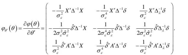
. In particular, ∆ = +ˆ I λˆZZ′ and ∆ = + I λZZ′. Let δ = −Y Xβ . The Wald statistic q can be obtained by Equa-tion (2) where the observed informaEqua-tion matrix evaluated at θˆ is

( )

( )

(

)

1 1 1

2 4 2

2

1 1 1

4 4 6 4

ˆ

2

1 1 1

2 4 2 1 2

1 _ˆ 1 _{ˆ ˆ} 1 _{ˆ ˆ}

ˆ ˆ ˆ

1 1 1

ˆ ˆˆ ˆˆ ˆ ˆˆ ˆ

ˆ 2ˆ ˆ 2ˆ

1 _ˆˆ 1 _{ˆˆ ˆ} 1 _{ˆˆ ˆ} 1

ˆ 2ˆ 2ˆ 2 ₁ ˆ

m _i i

i

X X X X

N j X n X n λ

ε ε ε

θθ λ

ε ε ε ε

θ

λ λ λλ

ε ε ε

δ δ

σ σ σ

θ

θ δ δ δ δ δ

θ θ σ σ σ σ

δ δ δ δ δ

σ σ σ _λ

− − − − − − ′ − − − =     ′∆ ′∆ − ′∆       ∂ ′ ′ ′ = − _′ = ∆ − + ∆ − ∆  ∂ ∂ _{ }   − ′∆ − ′∆ ′∆ −  +  

∑

  

where ∆ = ∂∆ ∂_λ−1 −1 λ and ∆ = − ∂ ∆ ∂−_λλ1 2 −1 λ2 are the first and second derivatives of ∆−1. The signed log-likelihood ratio statistic, r, defined in Equation (3) can be simplified to:

(

)

1 2

2 2

ˆ _ˆ ˆ

sign log log log log

r= λ λ− _N σ_ε + ∆ − N σ_ε − ∆_ (10)

calcu-lated by replacing θˆ=

(

β σ λˆ,ˆ_ε2,ˆ

)

in j_θθ′

( )

θˆ by the constrained maximum likelihood estimate θ=

(

β σ λ , _ε2,

)

. The usual form of the score test statistic is given by

( )

2 ₂

( )

1

2

S λ λ

λ λ −   ∂ ∂       =_{  }− _ ∂ ∂           _,

under the null hypothesis. Nuisance parameters are suppressed from notation. In the special case of testing zero variance component with n_i≡n, the score test statistic is ([12]):

(

)

2

₍

₎

2

2 1 1

1 1

with

2 2 1

m n ij i j C mn S C

nC mnσ_ε = =δ

−

= =

− _

∑ ∑

 .

Similar to the signed likelihood ratio test statistic, the signed score test statistic is:

( )

ˆ

sign

s=

λ λ

− S . (11)

Patterson and Thompson [6] proposed restricted or residual likelihood method which takes into account the loss of degrees of freedom involved in estimating the fixed effects and reduces the downward bias of maximum likelihood estimates of variance parameters. The restricted log-likelihood function is defined as

( )

2 1

(

)

1

(

)

2

1 1

log log log

2 2 2 2

RE N p Y X Y X

X X ε ε

β

β

θ

σ

σ

− − − ′∆ − − _′ = − − ∆ − ∆ −

 . (12)

The signed log-likelihood ratio statistic and Wald statistic with the restricted maximum likelihood can be ob-tained using the restricted log-likelihood function (Equation (12)) accordingly.

To obtain the third-order inference for λ, we need to find the canonical parameter ϕ θ

( )

. The canonical pa-rameter ϕ θ

( )

is approximated by taking the sample space gradient at the observed data point in the directions of a set of vectors V (Equation (7)):

( )

(

;y V

)

y

ϕ θ′ = ∂ θ ⋅

∂  .

where the sample space gradient is

(

;

)

(

2

)

1 21

y X

y

y _{ε ε}

β

δ

θ

σ

σ

− − ′ − ∆ ′ ∂ _{= − = −} ∆

∂  . (13)

Let ∆ =−1 L L′ . The tangent direction V is obtained from the pivotal quantity z y

(

;

θ

)

=L y

(

−X

β σ

)

_ε =L

δ σ

_ε (Equation (8)): 1 1 2 ˆ ˆ ˆ ˆ ˆ 2

z z L

V X L

y _{θ θ} ε λ λ

δ _δ

θ σ λ

− − = =   ∂   ∂   ∂  = −_{∂ ′} _{∂ ′} = −_ −  _∂  _    

   . (14)

Let A denotes 1

ˆ = L L λ λ λ − ∂     ∂

  in Equation (14). Multiply Equations (13) and (14), we have the canonical pa-

rameter

ϕ θ

′

( )

:

( )

(

)

21 212 12

ˆ ˆ , ˆ 2 X A y V

y _{ε ε ε ε}

δ δ δ δ δ

ϕ θ θ

σ σ σ σ

− − −

 ′ ′ ′ 

∂ ∆ ∆ ∆

′ = ⋅ =_ − _

∂  _{ }.

( )

( )

1 1 1

2 4 2

1 1 1

2 2 4 2 2 2

1 1 1

2 4 2

1 1 1

1 _ˆ 1 _ˆ 1 _ˆ

ˆ ˆ ˆ

2 2 2

1 _ˆ 1 _ˆ 1 _ˆ

X X X X

X

A X A A

λ

ε ε ε

θ λ

ε ε ε ε ε ε

λ

ε ε ε

δ δ

σ σ σ

ϕ θ

ϕ θ δ δ δ δ δ

θ σ σ σ σ σ σ

δ δ δ δ δ

σ σ σ

− − −

− − −

′

− − −

 

′ ′ ′

− ∆ − ∆ ∆

 

 

 

∂

′ ′ ′

= = − ∆ − ∆ ∆ 

′

∂ _{ }

 

 ′ ′∆ ′ ′∆ − ′ ′∆ 

 

 

.

Thus Q can be obtained by Equation (5) and we have the third-order approximations for λ _{by Equation (4).} All the equations and the maximizing problems can be programmed into R.

4. Application: A Real Data Example

We use a data set from the Genetic Analysis Workshop (GAW 18) to illustrate the application of our proposed method. The Genetic Analysis Workshops (www.gaworkshop.org), which began in 1982, were initially moti-vated by the development and publication of several new algorithms for statistical genetic analysis, using dif-ferent method of analysis. It is a collaborative effort among researchers worldwide to evaluate and compare sta-tistical genetic methods, relevant to current analytical problems in genetic epidemiology and stasta-tistical genetics. The GAW 18 data set [13] was drawn from the San Antonio Family Study (SAFS) with a total of 959 partici-pants from 20 families and it included the whole genome sequence data from all individuals. For each individual, age, sex, the use of hypertension diagnosis and antihypertensive medications (HTN) and tobacco smoking status (SMOKING) were recorded.

Our goal was to test the homogeneity of baseline systolic blood pressure (SBP) among families and if a ge-netic factor contributed to the variation of SBP among families. The test of homogeneity among families is a challenging task. The use of variance component of random effects in mixed models provides an efficient me-thod to account for the heterogeneity among families.

4.1. Test of Homogeneity of SBP among Families

We first evaluated the homogeneity of SBP levels among families using a random intercept mixed model. We analysed the SBP levels with “AGE” as fixed effect in a random intercept mixed model accounting for the va-riabilities of SBP among families. A non-zero variance of random intercept implies there exists a significant variation of SBP levels among families and the group specific random intercepts allow us to identify the families that deviate the most from the population average SBP levels at baseline.

Let y_ij denote the SBP measurements for the ith individual in the jth family, the linear mixed model formula for GAW 18 data with random intercept can be written as

0 0 1

ij j ij ij

y =β +b +βAGE +ε , (15)

where b_0j is the random intercept for the jth family.

[image:6.595.164.482.83.177.2]

To assess the variability of SBP, we obtain the 95% confidence interval of the variance component of random intercept λ. The 95% confidence intervals of λ obtained from third-order and first-order methods are recorded in Table 1. The third-order method yields a 95% confidence interval of

(

0.001, 0.0802 containing no zero, sug-

)

gesting a significant variation of SBP levels among families oppose to the results from first-order methods. The simulation studies have shown the superior accuracy of the third-order method and the conservativeness of the first-order methods. Thus we conclude that there is a significant variation of SBP among the 20 families based on the result from the third-order method. Figure 1(a) is the normal quantile plot of the random intercept b_0j

for the 20 families. The normal quanitle plot also confirms the variability of SBP levels among families.

4.2. Test of Homogeneity of SBP among Families in Relation to a Genetic Factor

Table 1. The 95% confidence intervals of λ, test homogeneity of SBP among families.

Method 95% CI

Third-order (0.001, 0.0802) LRT-REML (0, 0.0753)

[image:7.595.139.485.180.532.2]

LRT-ML (0, 0.0675) Wald-REML (0, 0.0503) Wald-ML (0, 0.0482) Score (0, 0.0488)

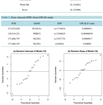
Table 2. Four selected SNPs from GWAS study.

POS GENE SNP GWAS P-value 127,074,020 PLXNA1 rs11716834 0.0000011 138,919,221 PISRT1 rs13100625 0.00000039 173,866,797 NLGN1 rs11927722 0.0000017 173,986,397 NLGN1 rs549641 0.00009

Figure 1. Normal quantile plots of random intercept for Model (15) and random slope for Model (16).

variables [14]. We use the average number of minor alleles from these four casual SNPs for each individual (denoted as grSNP_ij) was used as both as fixed effect and random slope in the model. To assess whether the effect of this combined genetic factor on SBP varies among families, we performed a test of variance component of the random slope in a random intercept and random slope mixed model. A non-zero variation of random slope implies significant variation of SBP levels among families due to the genetic factor. Backward elimination tech-nique was used for model selection and led to the following random intercept and random slope mixed model:

(

)

(

)

0 0 1 1 SNP 2AGE SEX SMOKING HTN SEX SMOKING HTN

ij j j ij ij ij ij ij ij

y =β +b + β +b gr +β + ∗ ∗ β _{∗ ∗} +ε (16)

where b_0j is the random intercept and b_1j is the random slope of the average number of minor alleles for the

jth family and

(

SEXij∗SMOKINGij∗HTNij

)

denotes the three-way interaction term including the lower order

and LRT-ML are (0.1035, 1.1008), (0.0554, 1.0445) and (0.0457, 0.9658) respectively. Not surprisingly, result from the likelihood ratio test methods are more conservative than with the third-order method.

Our two sets of analysis therefore demonstrated the interest of the third-order approach, the only method to find significant heterogeneity among families in terms of baseline SNP and change of SPB due to a combined genetic factor.

5. Simulation Studies

In this section, we present results from simulation studies for the random intercept mixed model and random in-tercept and random slope mixed model to assess the improvement of the third-order method and examine the accuracy of the proposed third-order method compared to the following first-order methods:

1) Third-order: the third-order method based on maximum likelihood;

2) LRT-REML: the signed log-likelihood ratio statistic method with restricted maximum likelihood estima-tion;

3) LRT-ML: the signed log-likelihood ratio statistic method with maximum likelihood estimation; 4) Wald-REML: Wald statistic with restricted maximum likelihood estimation.

5) Wald-ML: Wald statistic with maximum likelihood estimation; 6) Score: Score test with maximum likelihood estimation.

The statistical software R (“nlme” package) was used to carry out all our analyses.

5.1. Simulation Results for the Random Intercept Mixed Model

We present simulation results for the null distribution of the zero variance component λ: H₀:λ =0

(

σ_b2=0

)

versus Ha:λ >0

(

)

2

0

b

σ > and for non-zero variance component λ: H₀:λ =4 versus Ha:λ >4 in a

random intercept mixed model.

5.1.1. H0:λ=0 versus Ha:λ>0

Balanced data sets with equal group size ni = =n 10 were generated with fixed effect β =

(

β β0, 1

) ( )

= 1, 2 ,

2

1

ε

σ

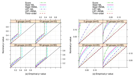
= for the test of zero variance compoennt λ = 0. For each simulation configuration, 10,000 iterations were used for a number of groups m = 5, 10, 20, 50.

Probability-probability plots (pp-plot), similar to a quantile-quantile (qq-plot) but on the p-value scale rather than on the scale of the test statistic [6], are used to examine the accuracy of the p-values obtained from the six methods. For a perfect approximation, the p-values line up on the 45˚ diagonal line. The nominal p-values cal-culated from the six methods, are plotted versus the empirical p-values in Figure 2(a). Figure 2(b) shows only the 0 to 15th percentile ofFigure 2(a), that allows us have a clearer look at the differences. Figure 2shows that when group size n = 10, the third-order method is surprisingly accurate and consistent regardless of the number of groups m. The likelihood ratio test is the most accurate among the first-order methods while the likelihood ra-tio test with restricted maximum likelihood estimara-tion reduces the bias of maximum likelihood estimara-tion. The approximations from Wald test and score test are poor, thus omitted for the rest of this paper. The figures also show that the proportion of point mass at 0 converges to 50% when sample size increases.

To further examine the accuracy of the third-order and first-order approximations, a 3-dimensional plot is used to visualize the bias for a number of groups m varying from 3 to 40 and group size n from 5 to 40 (Figure 3). The bias is calculated by subtracting the nominal p-value at the 5th percentile from its empirical (or true)

p-value 0.05. A bias of zero implies perfect approximation and a positive bias implies conservativeness (greater than the true p-value). Figure 3 shows the same pattern asFigure 2: the third-order method is accurate and con-sistent. The likelihood ratio test with restricted maximum likelihood estimation is more accurate than that of maximum likelihood estimation. We observe an interesting pattern that is for a given number of groups m, the bias is small when the group size n is small, it increases with group size n and then flattens down and decreases slowly. For a given number of group size n, the bias decreases with m. The phenomenon suggests that the accu-racy of first-order methods depend on both number of groups m and the group size n.

5.1.2. H0:λ=4 versus Ha:λ>4

In this section, we show simulation results for a non-zero variance component H₀:λ =4 versus Ha:λ >4.

[image:9.595.83.537.79.338.2]

Figure 2. Probability-probability plot for testing λ = 0 vs. λ > 0 for number of groups m = 5, 10, 20, 50 with equal group size n = 10. For a perfect approximation, the p-values line up on the 45˚ diagonal line. This plot shows the conservativeness of the first-order methods.

Figure 3. 3-D bias plots testing λ = 0 vs. λ > 0 for various number of groups m and group size n. The bias is calculated subtracting the nominal p-value from the five methods at the 5th percentile from its empirical (or true) p-value 0.05. A bias of zero implies perfect approximation and a positive bias implies that the approximation is conservative (greater than the true p-value).

2

1

ε

σ

= and λ = 4. For each simulation configuration, 10,000 iterations were used for a number of groups m = 5, 10, 20, 50. Again, the pp-plot inFigure 4 confirms the superior accuracy of the third-order method.

[image:9.595.93.534.384.551.2]

[image:10.595.202.428.84.319.2]

Figure 4. Probability-probability plot for testing λ = 4 vs. H_a:λ>4 for number of groups m = 5, 10, 20, 50 with equal group size n = 10.

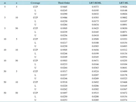
Table 3.Central coverage probabilities and error probabilities for testing H₀:λ=4 versus H_a:λ>4. The nominal val-ues are 0.95 0.025, 0.025 with standard errors 0.0022, 0.0016 and 0.0016 for CCP, L and U respectively.

m n Coverage Third-Order LRT-REML LRT-ML

5 5 CCP 0.9465 0.9373 0.9026

L 0.0245 0.0195 0.0148

U 0.0290 0.0432 0.0826

5 10 CCP 0.9486 0.9393 0.9002

L 0.0230 0.0173 0.0107

U 0.0284 0.0434 0.0891

5 50 CCP 0.9505 0.9425 0.9030

L 0.0239 0.0165 0.0071

U 0.0256 0.0410 0.0899

10 5 CCP 0.9553 0.9509 0.9353

L 0.0217 0.0188 0.0154

U 0.0230 0.0303 0.0493

10 10 CCP 0.9505 0.9456 0.9312

L 0.0246 0.0199 0.0134

U 0.0249 0.0345 0.0554

10 50 CCP 0.9503 0.9471 0.9255

L 0.0233 0.0166 0.0104

U 0.0264 0.0363 0.0641

50 5 CCP 0.9517 0.9524 0.9499

L 0.0237 0.0207 0.0178

U 0.0246 0.0269 0.0323

50 10 CCP 0.9518 0.9492 0.9468

L 0.0220 0.0206 0.0165

U 0.0262 0.0302 0.0367

50 50 CCP 0.9497 0.9515 0.9472

L 0.0250 0.0200 0.0154

[image:10.595.89.538.387.723.2]

0.0022, 0.0016 and 0.0016, respectively. The table shows that the third-order method has the best coverage probabilities. It is always accurate with symmetric lower and upper error coverage probabilities. The LRT- REML has good central coverage probabilities in some cases however the lower and upper coverage probabili-ties are asymmetric with the lower error probabiliprobabili-ties tends to be less than the true value and the upper probabil-ities tend to be larger.

5.2. Simulation Results for Random Intercept and Random Slope Mixed Model

Testing zero variance component of random slope in a random intercept and random slope mixed model implies that we are testing both λ01 = 0 and λ11 = 0. The third-order method is currently limited to the test of a scalar

pa-rameter. Theoretical development for vector parameter using third-order approach has not been proposed yet. Instead of testing λ11 = 0, we could obtain the 95% confidence interval of λ11. Thus we show the the simulation

results for the test of a non-zero variance component of random slope H₀:λ =₁₁ 4 versus Ha:λ >₁₁ 4. We

generated balanced data sets with equal group size ni= =n 10 with fixed effect β =

(

β β0, 1

) ( )

= 1, 2 , 2

1 ε

σ = ,

λ00 = 1, λ01 = 1 and λ11 = 4, and a number of groups m = 5, 10, 20, 50. For each simulation configuration,

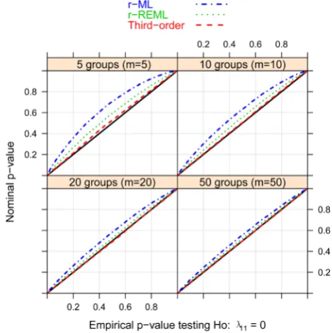
10, 000 iterations were used. Figure 5 is the pp-plot for H₀:λ =₁₁ 4 versus Ha:λ >₁₁ 4. The third-order

method has shown its superior accuracy and symmetric tail probabilities for the test of variance component of random slope in a random intercept and random slope mixed model. The LRT with REML is less conservative than LRT with ML.

In this section, we presented simulation results for the tests of variance component in linear mixed models. The simulation results demonstrated that the third-order method is accurate and consistent. The LRT method perform the best among all first-order methods and the REML reduce the bias comparing the ML. The computa-tion time for third-order p-values is fast and depends on sample size. It takes only a few seconds for a sample of 40 group with group size of 40 on a personal computer with a Quad CPU @3 GHz and 8 GB RAM .

6. Discussion

[image:11.595.195.430.458.694.2]

A third-order likelihood-based method is proposed for the tests of zero and non-zero variance component in the random intercept mixed model and the random intercept and random slope mixed model. The third-order me-thod requires only the observed likelihood function and derivation of the pivotal quantity and ancillary direction. The computation of third-order method is efficient. Our simulation studies show that the proposed third-order

likelihood-based method provides substantial improvement over traditional first-order methods. It provides ex-tremely accurate and consistent approximation for the tests of variance component in mixed models even when the number of groups and group sizes are as small as five and three respectively. The likelihood ratio test per-forms the best among the first-order methods. The likelihood ratio test with restricted maximum likelihood es-timation is less conservative than the maximum likelihood eses-timation. The likelihood ratio test with restricted maximum likelihood estimation is recommended for the test of variance component in mixed models whenever the first-order method is used. The application to the GAW 18 data illustrated the advantages of the third-order methods for the test of homogeneity among families in relation to a genetic factor. The simulation results also yielded a comprehensive evaluation of the accuracy of the first-order methods. The third-order method provides also opportunities for further applications in the context of longitudinal studies with repeated measurements and genetic studies. For example, there has been increased interest in genetic analysis to test the combined effect of several rare variants using random effects in the mixed model framework [14]. Since some popular approaches for this type of analysis are based on the score test of random effect, we think that the third-order approach could provide a more accurate alternative in this context, that we are planning to explore in future work.

References

[1] Britton. T. (1997) Tests to Detect Clustering of Infected Individuals within Families. Biometrics, 53, 98-109. http://dx.doi.org/10.2307/2533100

[2] Liang, K.Y. (1987) A Locally Most Powerful Test for Homogeneity with Many Strata. Biometrics, 51, 259-264. http://dx.doi.org/10.1093/biomet/74.2.259

[3] Chernoff, H. (1954) On the Distribution of the Likelihood Ratio. Annals of Mathematical Statistics, 25, 573-578. http://dx.doi.org/10.1214/aoms/1177728725

[4] Self, S.F. and Liang, K.Y. (1987) Asymptotic Properties of Maximum Likelihood Estimator and Likelihood Ratio Tests under Nonstandard Conditions. Journal of the American Statistical Association, 82, 605-610.

http://dx.doi.org/10.1080/01621459.1987.10478472

[5] Stram, D.O. and Lee, J.W. (1994) Variance Components Testing in the Longitudinal Mixed Effects Model. Biometrics,

50, 71171-1177. http://dx.doi.org/10.2307/2533455

[6] Patterson, H.D. and Thompson, R. (1971) Recovery of Interblock Information When Block Sizes Are Unequal. Biome-trika, 58, 545-554. http://dx.doi.org/10.1093/biomet/58.3.545

[7] Crainiceanu, D.M. and Ruppert, D. (2004) Likelihood Ratio Tests in Linear Mixed Models with One Variance Com-ponent. Journal of the Royal Statistical Society: Series B, 66, 165-185.

http://dx.doi.org/10.1111/j.1467-9868.2004.00438.x

[8] Fraser, D.A.S., Reid, N. and Wu. J. (1999) A Simple General Formula for Tail Probabilities for Frequentist and Baye-sian Inference. Biometrika, 86, 249-264. http://dx.doi.org/10.1093/biomet/86.2.249

[9] Barndorff-Nielsen, O.E. (1986) Inference on Full and Partial Parameters, Based on the Standardized Signed Log-Like- lihood Ratio. Biometrika, 73, 307-322. http://dx.doi.org/10.2307/2336207

[10] Barndorff-Nielsen, O.E. (1991) Modified Signed Log-Likelihood Ratio Statistic. Biometrika, 78, 557-563. http://dx.doi.org/10.1093/biomet/78.3.557

[11] Fraser, D.A.S. and Reid. M. (1995) Ancillaries and Third-Order Significance.Utilitas Mathematica, 47, 33-53. [12] Verbeke, G. and Molenberghs, G. (2003) The Use of Score Tests for Inference on Variance Components. Biometrics,

59, 254-262. http://dx.doi.org/10.1111/1541-0420.00032

[13] Almasy, L., Dyer, T.D., Peralta, J.M., Jun, G., Fuchsberger, C., Almeida, M.A., Kent, J.W., Fowler, S., Duggirala, R. and Blangero. J. (2014) Data for Genetic Analysis Workshop 18: Human Whole Genome Sequence, Blood Pressure, and Simulated Phenotypes in Extended Pedigrees. BMC Proceedings, 8, S2.