Improved Task Scheduling on Parallel System
using Genetic Algorithm
Jasbir Singh
Department of Computer Science and IT, Guru
Gobind Singh Khalsa College, Sarhali (Tarn
Taran), Punjab-India
Gurvinder Singh
Department of Computer Science and
Engineering, Guru Nanak Dev University
(Amritsar), Punjab, India
ABSTRACT
Parallel Processing refers to the concept of speeding-up the execution of a task by dividing the task into multiple fragments that can execute simultaneously, each on its own processor i.e. it is the simultaneous processing of the task on two or more processors in order to obtain faster results. It can be effectively used for tasks that involve a large number of calculations, have time constraints and can be divided into a number of smaller tasks. The scheduling problem deals with the optimal assignment of a set of tasks onto parallel multiprocessor system and orders their execution so that the total completion time is minimized. The efficient execution of the schedule on parallel multiprocessor system takes the structure of the application and the performance characteristics of the proposed algorithm. Many heuristics and approximation algorithms have been proposed to fulfill the scheduling task. It is well known NP-complete problem. This study proposes a genetic based approach to schedule parallel tasks on heterogeneous parallel multiprocessor system. The scheduling problem considered in this study includes - next to search for an optimal mapping of the task and their sequence of execution and also search for an optimal configuration of the parallel system. An approach for the simultaneous optimization of all these three components of scheduling method using genetic algorithm is presented and its performance is evaluated in comparison with the First Come First Serve (FCFS), Shortest Job First (SJF), Round Robin (RR), Priority and Largest Job First (LJF) scheduling methods.
Key words
Parallel Multiprocessor System, Directed Acyclic Graph (DAG), simultaneous optimization, Genetic Algorithm.
1. INTRODUCTION
Task assignment and scheduling [1][2][3][4] can be defined as assigning the tasks onto a set of processor and determining the sequence of execution of the task at each processor. While the total finish time of the tasks is determined by the performance of the processors and the sequence of the tasks, therefore, an execution scheduling consists of three components:
Performance of the heterogeneous processor
Mapping of the tasks onto the processors
Sequence of the execution of the tasks on each processor
All three components of this optimization problem [5][30] are highly dependent on each other and should not be optimized separately.
A Genetic Algorithm (GA) approach is being proposed to handle the problem of parallel system task scheduling. A GA [7][8] starts with a generation of individual, which are encoded as strings known as chromosome. A chromosome corresponds to a solution to the problem. A fitness function is used to evaluate the fitness of each individual. In general, GAs consists of selection, crossover and mutation operations [15] based on some key parameters such as fitness function, crossover probability and mutation probability.
This study is divided into following sections: In section 2 an overview of the problem is given along with brief description of the solution methodology. Section 3 provides a detailed improved parallel genetic algorithm. Experimental results and performance analysis are provided in section 4 and conclusion is followed in section 5.
2. PROBLEM DEFINITION
Parallel Multiprocessor system scheduling can be classified into many different classes based on the characteristics of the tasks to be scheduled, the multiprocessor system and the availability of the information[6][9][11][12][13][14]. The strategy behind the execution of the tasks on parallel multiprocessor system environment is to efficiently partitioning the huge task into set of tasks of appropriate gain size and an abstract model of the partitioned tasks that can be represented by Directed Acyclic Graph (DAG)[25][28][29]. The focus is on a deterministic scheduling problem in which there exist precedence relations among the tasks to be scheduled. A deterministic scheduling problem [16] is one in which all information about the tasks and the relation to each other such as execution time and precedence relation are known to the scheduling algorithm in advance and the processor environment is heterogeneous[23][24][26][27]. Heterogeneity of processors means that the processors have different speeds or processing capabilities.
In this study, a study has been done regarding the task scheduling problem as a deterministic on the heterogeneous multiprocessor environment. The main objective is to minimize the total task finish time (execution time + waiting time or idle time).
The multiprocessor computing environment consists of a set of m heterogeneous processor:
They are fully connected with each other via identical links. Figure 1 shows a fully connected eight parallel system with identical link.
[image:2.595.99.247.114.245.2]
Fig. 1: A fully connected parallel processor
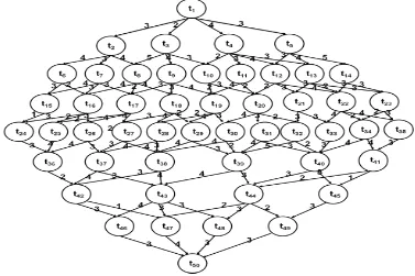
The parallel application can be represented by a directed acyclic graph (DAG), G = (T, E, W, C), where the vertices set T consist of n tasks as:
T = {tj: j =1, 2, 3…n}
A directed edge set E consist of k edges as: E = {ek: k =1, 2, 3…r}
This represents the precedence relationships among tasks. For any two tasks ti, ti+1 Є T with having directed edge ek
(i.e., edge from task ti to ti+1) means that task ti+1 cannot be
scheduled until ti has been completed, ti is a predecessor of
ti+1 and ti+1 is a successor of ti. In other words ti sends a
message whose contents are required by ti+1 to start
execution.
The elements set W are the weights of the vertices as: W = {wi,j: i =1, 2, 3…m, j: 1, 2, 3,…n}
It represents the execution duration of the corresponding task and are varies from processor to processor because of heterogeneous processor environment.
The elements set C are the weights of the edges as: C = {ck: k =1, 2, 3…r}
It represents the data communication between the two tasks, if they are scheduled to different processors. But if both tasks are scheduled to the same processor, then the weight associated to the edge becomes null. Figure 2 show example of DAGs. It consist of a set of tasks T: {tj: j = 1, 2
…}, Fig. 1 indicates set of processors P = {pi : i = 1, 2,
3…} and Table 1 show a matrix of execution time of each task on processor p1, p2, p3, p4, p5, p6, p7, p8, because of
heterogeneous environment every processor works on different speeds and processing capabilities. It is assumed that processor p1 is much faster than p2, p3 and so on.
Processor p2 is faster than p3, p4 and so on. (i.e., the order
of speed and processing capabilities can be expressed as p1>p2> p3 > p4 > p5 > p6 > p7>p8). As given in Table 1
task t1 takes 4 time units to complete their execution on
processor p1 and takes 8 time units and 9 time units to
complete their execution on processor p7 and p8
respectively. This execution time has been calculated on the basis of the size of the tasks by processing on different processors.
[image:2.595.96.473.457.708.2]t1 t2 t3 t4 t5 t6 t7 t8 t9 t10 t11 t12 t13 t14 t15 t16 t17 t18 t19 t20 t21 t22 t23 t24 t25 t26 t27 t28 t29 t30 t31 t32 t33 t34 t35 t36 t37 t38 t39 t40 t41 t42 t43 t44 t45 t46 t47 t48 t49 t50
p1 4 3 6 5 2 8 7 4 9 10 11 6 12 13 10 16 10 7 6 3 9 12 13 15 7 10 6 8 4 5 6 7 10 13 9 12 10 4 3 8 11 9 12 2 14 13 9 7 10 9
p2 4 4 7 6 3 9 8 5 10 11 12 6 13 13 11 17 10 8 7 4 10 13 13 15 8 10 6 9 5 6 6 8 11 14 10 12 10 5 4 9 12 10 13 2 14 13 10 8 11 10
p3 5 5 7 7 3 9 9 5 10 11 12 7 15 14 12 18 11 8 8 5 10 13 14 17 8 11 7 9 6 6 7 8 12 14 10 13 11 5 4 9 12 11 13 3 16 14 11 9 11 11
p4 6 5 8 7 4 10 9 6 11 12 14 8 16 15 13 18 11 9 8 5 11 14 14 17 9 12 8 10 7 7 8 9 14 16 11 15 12 6 5 10 13 12 14 3 16 14 11 10 12 12
p5 7 6 9 8 4 11 10 6 11 13 14 9 17 16 14 20 12 10 9 6 12 15 15 18 10 13 9 11 7 8 9 10 14 17 12 15 13 6 5 10 15 13 15 4 17 16 13 11 13 13
p6 7 7 10 8 5 11 10 7 12 14 15 10 19 18 15 20 13 11 10 6 13 16 15 18 11 14 10 12 8 8 10 11 15 18 13 16 13 7 6 11 15 14 15 4 17 16 14 11 14 13
p7 8 7 10 9 5 12 11 8 13 14 16 10 19 19 15 22 14 12 10 7 14 16 16 20 12 15 10 13 8 9 11 12 16 19 14 17 14 8 6 12 16 15 16 5 18 17 15 12 15 14
p8 9 8 11 10 6 12 11 9 13 15 16 11 20 19 16 22 14 13 11 7 14 17 17 20 13 15 11 14 9 10 12 13 17 20 15 18 15 8 7 13 16 16 17 5 19 18 16 13 15 15
Table 1: Shows a tasks execution matrix on different processors with task size = 50.
3. PERFORMANCE EFFECTIVE
GENETIC ALGORITHM
GAs operate through a simple cycle of stages: creation of a population strings, evaluation of each string, selection of the best strings and reproduction to create a new population. The individuals are encoded in the population string known as chromosomes. Once the chromosome has been coded, it is possible to evaluate the performance or fitness of individuals in a population. A good coding scheme [17][18] will benefit operators and make the object function easy to calculate.
During selection, each individual is assigned a fitness value given by the objective function and choose the fittest individual of the current population to serve as parent of the next generation. Reproduction involves two types of operators namely crossover and mutation.
The crossover operator chooses randomly a pair of individuals among those selected previously and exchange some part of the information. The mutation operator takes an individual randomly and alters it.
A. Creation of the population string: The first step in the GAs algorithm is the creation of the initial population. Number of processors, number of tasks and population size are needed to generate initial population. The initial population is initialized with randomly generated individuals. The length of all individuals in an initial population is equal to the number of tasks in the DAG. Each task is randomly assigned to a processor.
B. Evaluation of the fitness function: The fitness function used for improved parallel genetic algorithm is based on the total completion time for the schedule, which includes execution time and communication delay time.
Table 2a: Random assignment of tasks to parallel
processors (Valid order)
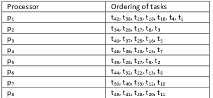
Table 2(b): Random assignment of tasks to parallel processors (Invalid order), because no processor (p1, p2,
p3……p8) starts execution of tasks t42, t34, t40 t46, t39, t44,
t50, t49 respectively until the execution of task t1. The
tasks t42, t34, t40 t46, t39, t44, t50, t49 required information
from t1 to start their execution.
The fitness function separates the evaluation into two parts: Task fitness and processor fitness. The task fitness focuses on ensuring that all tasks are performed and scheduled in valid order. A valid order means that a pair of tasks is independent if neither task get data output from the other task for execution. The scheduling of a pair of tasks to a single processor is valid if the pair is independent or if the order in which they are assigned to the processor matches the order of their dependency. Table 2 (a) show a valid order of the tasks assigned to the set of processors (p1, p2, p3……) and invalid order in Table 2 (b).
The processor fitness component of the fitness functionattempts to minimize processing time. Consider the following schedule S1 and S2 for single processor and multiprocessor parallel system tasks schedules with task size equal to 50 tasks respectively (here, we consider the case when fitness function assigned all tasks to a single processor and randomly generated tasks to heterogeneous parallel system.) The processor chosen for scheduler S1 is p1 and the execution time for all task are given in Table 1.
The total finish time of scheduler S1 and S2 is:
S1: t1 t2 t3 ---t49 t50
Total Finish Time = Execution time + Comm. time. =4+3+6+5+2+8+7+4+9+10+11+6+12+13+10+16+10+7+6 +3+9+12+13+15+7+10+6+8+4+5+6+7+10+13+9+12+10+ 4+3+8+11+9+12+2+14+13+9+7+10+9 =419time units
Processor Ordering of tasks
p1 t42, t38, t23, t18, t16, t4, t1
p2 t34, t28, t17, t6, t3
p3 t40, t37, t25, t16, t5
p4 t46, t36, t23, t15, t7
p5 t39, t28, t17, t9, t2
p6 t44, t32, t22, t13, t8
p7 t50, t40, t33, t12, t10
p8 t49, t41, t28, t20, t11
Processor Ordering of tasks
p1 t1, t4, t11, t8, t16, t24, t40, t45, t49, t50 . p2 t2, t13, t21, t31, t30, t25, t37, t43, t47. p3 t10, t20, t18, t32 t34, t41, t44, t48. p4 t5, t14, t22, t33, t36, t42, t46. p5 t6, t19, t29, t26, t36, t42, t46. p6 t9, t17, t27, t39.
[image:3.595.338.550.351.449.2]Here comm. Time = 0, because all tasks are executed on same processor.
Figure 3: A Gantt chart for Scheduler S2.
The processors chosen for schedule S2 are same as given in table 1 and the randomly order sequence is given in table 2 (a). The Gantt chart for scheduler S2 is shown in figure 3.
In figure 3, the symbol # represents the execution time of the task on the corresponding processor (for example t1 (4)
means, the execution time of task t1 is 4 time units on
processor p1.) and * represent the communication time or
idle time (for example, in figure 3, (7)* means task t2
cannot start execution until t1 compete their execution.
S2: Total finish time = Execution time + Comm. Time = 118 time units
The scheduler S1 shows a total finish time of 419 time units, where as scheduler S2 shows a total finish time of just 118 time units. Therefore, proper fitness function reduces the total finish time very well.
Therefore, the fitness values (task & processor) have been evaluated for all chromosomes and the probability of higher fitness is to be selected for reproduction from current generation to the next generation.
C. Selection operator: The design of the fitness function is the basic of selection operation, so how to design the fitness function will directly affect the performance of genetic algorithm. GAs uses selection operator to select the superior and eliminate the inferior. The individual are selected according to their fitness value. Once fitness values have been evaluated for all chromosomes, we can select good chromosomes through rotating roulette wheel strategy. This operator generate next generationby selecting best chromosomes from parents and offspring.
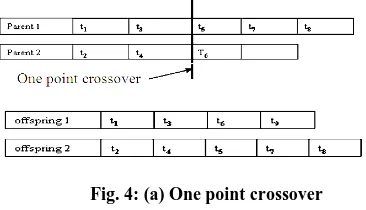
D. Crossover operator: Crossover operator randomly selects two parent chromosomes (chromosomes with higher values have more chance to be selected) and randomly chooses their crossover points, and mates them to produce two child (offspring) chromosomes. We examine one and two point crossover operators. In one point crossover, the segments to the right of the crossover points are exchanged to form two offspring as shown in Fig. 4(a) and in two point crossover [19][20], the middle portions of the crossover points are exchanged to form two offspring as shown in Fig. 4(b).
Randomly selects parent 1 and 2, crossover point 2:
Fig. 4: (a) One point crossover
Randomly selects parent 1 and 2, crossover points 1 and 3:
Fig. 4: (b) Two point crossover
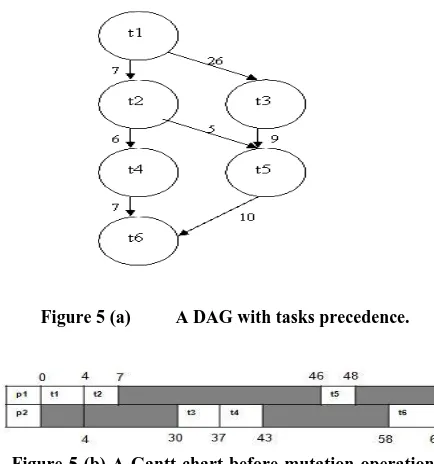
Mutation operator: A mutation operation is designed to reduce the idle time of a processor waiting for the data from other processors. It works by randomly selecting two tasks and swapping them. Firstly, it randomly selects a processor, and then randomly selects a task [21] on that processor. This task is the first task of the pair to be swapped. Secondly, it randomly selects a second processor (it may be the same as the first), and randomly selects a task. If the two selected tasks are the same task the search continues on. If the two tasks are different then they are swapped over (provided that the precedence relations must satisfy). Consider the following example of six tasks DAG with tasks precedence and the execution times of tasks t1 to t6 on processor p1 and p2 are given in
[image:4.595.331.514.293.398.2] [image:4.595.349.528.437.533.2]Figure 5 (a) A DAG with tasks precedence.
Figure 5 (b) A Gantt chart before mutation operation, which takes 67 time units to complete the schedule.
Figure 5 (c) A Gantt chart after mutation operation, which takes 36 time units to complete the schedule
Here the mutation operation swaps task t2 on processor p1
to task t3 on processor p2.
The procedure of the Genetic Algorithm (GA) is:
Step 1: Setting the parameter
Set the parameter: Read DAG (task execution matrix (number of tasks n, number of processors m) and comm. cost), population size pop_size, crossover probability pc, mutation
probability pm, and maximum generation
maxgen
Let generation gen = 0, maxeval = 0 Step 2: Initialization
Generate pop size chromosomes randomly. Step 3: Evaluate
Step 3.1: Calculate the fitness value of each chromosomes
Step 3.2: Task fitness Step 3.2: Processor fitness Step 4:Crossover
Perform the crossover operation on the chromosomes selected with probability pc.
Step 5: Mutation
Perform the swap mutation on chromosomes selected with probability pm.
Step 6: Selection Select pop_size chromosomes from the parents and offspring for the next generation
Step 7: Stop testing If gen = maxgen, then output best solution and stop else gen = gen + 1 and return to step 3
4. EXPERIMENTAL RESULTS AND
PERFORMANCE ANALYSIS
The final best schedule obtained by applying the Genetic Algorithm (GA) to the DAG of Fig. 2 with execution time shown in Table 1 onto the parallelmultiprocessor system is shown in Fig. 6.
Fig. 6:Time taken to complete the schedule by GA, SJF, FCFS, RR, Priority and Largest Job First (LJF) Scheduler on parallel multiprocessor system for task size = 50tasks
We also compare the results with Shortest job First (SJF), First Come First Serve (FCFS), Round Robin (RR), Priority and Largest Job First (LJF) scheduling method [22] on parallel systems and execution of the schedules are shown in Fig. 7 for task size equal to 50.
A. Performance analysis: Speed up (Tsp): Speed up[22]
is defined as the completion time on a uniprocessor divided by completion time on a multiprocessor. In case of homogeneous system, it is denoted as: Tsp = p(1)/p(m). But
in case of heterogeneous system, it is denoted as Tsp= (min
[image:5.595.72.289.57.289.2](p(1)) / p(m) i.e., the best uniprocessor completion time divided by the completion time on a heterogeneous multiprocessor system. The speedup is measured with the execution of tasks on single processor which shows 419 time units for task size equal 50 tasks divided by execution time units on GA, SJF, FCFS, Round Robin (RR), Priority and Largest Job First (LJF) scheduler as shown in Fig. 7.
Fig. 7: Speedup v/s number of parallel
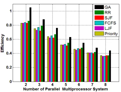
[image:5.595.317.551.137.325.2] [image:5.595.328.554.579.762.2]B. Efficiency (¢): (Tsp / m), where m is the number of
processors.
Fig. 8: Performance comparisons of the GA, SJF, FCFS, RR, Priority and LJF for task size = 50tasks
5. CONCLUSION
In this study we have proposed Genetic Algorithm (GA) for task scheduling in heterogeneous parallel multiprocessor system to minimize the finish time including execution time and waiting or idle time and increase the throughput of the system. The proposed method found a better solution for assigning the tasks to the heterogeneous parallel multiprocessor system. Experimental results and Genetic Algorithm is compared with FCFS, SJF, Round Robin (RR), Priority and Largest Job First (LJF) scheduling methods. The performance study is based on the best randomly generated schedule of the Genetic Algorithm.
6. REFERENCES
[1] Sara Baase, Allen Van Gelder,”Computer Algorithms”, Published by Addison Wesley, 2000. [2] Sartaj Sahni, ”Algorithms Analysis and Design”,
Published by Galgotia Publications Pvt. Ltd., New Delhi, 1996.
[3] Anup Kumar, Sub Ramakrishnan, Chinar Deshpande, Larry Dunning, “ IEEE Conference on Parallel processing”, 1994Page no.83-87.
[4] Ananth Grama, Georage Karypis, Anshul Gupta, Vipin Kumar,“Introduction to parallel computing”, Published by Pearson Education, 2009.
[5] Kalyanmoy Deb,”Optimization for Engineering Design”, Published by PHI, 2003.
[6] Dezso Sima, Terence Fountain, Peter Kacsuk, “ Advanced Computer Architectures”, Published by Pearson Education, 2009.
[7] David E. Goldberg,”Genetic Algorithms in Search, Optimization and Machine Learning”, Published by Pearson Education, 2004, Page No.60-83.
[8] Mitchell, Melanie,” An Introduction to Genetic Algorithm, Published Bu MIT Press 1996
[9] Michael J Qumn, “Parallel Computing Theory and Practices, 2nd Edition”, Published by Tata McGraw Hill Education Private Ltd, Page No. 346-364.
[10] Michael J Qumn, “Parallel Programming”, Published by Tata McGraw Hill Education Private Ltd, Page No. 63-89.
[11]John L Hennessy, David A Pattern, “Computer Architecture, 3rd Edition”, Published by Morgan Kaufmann & Elsevier India, Page No. 528-590. [12]David E Culler, “Parallel Computer Architecture”,
Published by Morgan Kaufmann & Elsevier India. [13]J P Hayes, “Computer Architecture and
Organization”, Published by McGraw Hill International Edition.
[14]J D Carpinalli, “Computer System Organization & Architecture”, Published by Pearson Education. [15]Sung-Ho Woo, Sung-Bong Yang, Shin-Dug Kim, and
tack-Don Han ,” IEEE Trans on parallel System, 1997, Page 301-305.
[16]M.Salmani Jelodar, S.N.Fakhraie, S.M.fakharie, M.N. Ahmadabadi,” IEEE Proceeding, 2006, Page No 340-347.
[17]Man Lin and Laurence tianruo Yang,”IEEE Proceeding”, 1999, Page No 382-387
[18]Yajun Li, Yuhang yang, Maode Ma, Rongbo Zhu, “ IEEE Proceeding”, 2008.
[19]YI-Wen Zhong, Jian-Gang Yang, Heng-Nlan QI,” IEEE Proceeding”, August 2004, Page No. 2463-2468.
[20]Imtiaz Ahmad, Muhammad K. Dhodhi and Arif Ghafoor,” IEEE Proceeding”, 1995, Page No. 49-53. [21]Ceyda Oguz and M.Fikret Ercan,” IEEE Proceeding”,
2004, Page No. 168-170
[22]Kai Hwang & Faye A. Briggs,”Computer Architecture and Parallel Processing”, Published by McGraw Hill ,1985.Page No. 445-47, 612.
[23]Andrei R. & Arjan J.C. van Gemund, “Fast and Effective Task Scheduling in Heterogeneous Systems”, IEEE Proceeding, 2000.
[24]Michael Bohler, Frank Moore, Yi Pan, “Improved Multiprocessor Task Scheduling Using Genetic Algorithms”, Proceedings of the Twelfth International FLAIRS Conference, 1999.
[25]Andrew J. page,” Adaptive Scheduling in Heterogeneous Distributed Computing System”, [26]Jameela Al-Jaroodi, Nader Mohamed, Hong Jiang
and David Swanson,” Modeling Parallel Applications Performance on Heterogeneous Systems”, Proceedings of the International Parallel and Distributed Processing Symposium (IPDPS’03) [27]Yu-Kwong and Ishraq Ahmad, “Static Scheduling
Algorithms for Allocating Directed Task Graphs to Multiprocessors”, ACM Computing Surveys, Vol. 31, No. 4, December 1999
[28]Wai-Yip Chan and Chi-Kwong Li, “Scheduling Tasks in DAG to Heterogeneous Processor System”, Proceeding IEEE 1998.
[29]Wojciech Cencek, “High-Performance Computing on Heterogeneous Systems”, Computational Methods in Science and Technology, 1999
[image:6.595.52.295.109.295.2]