Structural Time Series Modelling of Capacity Utilisation

Munich Personal RePEc Archive

Structural Time Series Modelling of

Capacity Utilisation

Proietti, Tommaso

Università di Udine

6 June 1999

S

TRUCTURAL

T

IME

S

ERIES

M

ODELLING OF

C

APACITY

U

TILISATION

Tommaso Proietti

Dipartimento di Scienze Statistiche,

Universit`a di Udine

Via A. Treppo, 18, 33100 Udine, Italy

E-mail proietti@dss.uniud.it

Tel. +39 0432 249581; Fax: +39 0432 249595

A

BSTRACT

In this paper we introduce a structural non-linear time series model for joint

esti-mation of capacity and its utilisation, thereby providing the statistical underpinnings to

a measurement problem that has received ad hoc solutions, often underlying arbitrary

assumptions. The model we propose is a particular growth model subject to a

satura-tion level which varies over time according to a stochastic process specified a priori. A

bivariate extension is discussed which is relevant when survey based estimates of

utiliza-tion rates are available. Illustrautiliza-tions are provided with respect to the US and the Italian

industrial production.

Key words: Structural Time Series Models, Nonlinear models, Extended Kalman Filter,

1

Introduction

The measurement of productive capacity and its utilization has attracted a lot of attention

in the economic and statistic literature. Since it deals with an artificial construct, its

do-main is rather controversial, and it is not surprising that different methods of measurement

have been proposed, each appealing to economic theory in different degrees.

This article does not aim at reviewing this literature, mostly because excellent

re-views are already available, such as Christiano’s (1981). The recent additions mainly

deal with the related issue of measuring potential output for the aggregate economy, and

are paced to the developments in the econometric analysis of time series. For instance,

DeSerres et al. (1995) measure potential output within a structural VAR framework, as

the output dynamics produced by permanent supply and oil shocks; other bivariate work

exploits either the Okun Law or the Phillips Curve relationships, according to which the

output gap is related to the unemployment rate and to inflation, respectively; see Evans

(1989), Clark (1989), Kuttner (1994) and Norden (1995). The latter uses an observable

index model (Sims and Sargent, 1977), whereas the others treat potential output as a latent

variable.

In this article we propose a measurement method that is quite neutral in that it

does not necessarily assume a particular definition of capacity; perhaps it is closer to an

engineering concept, for which capacity is defined as the as the maximum output that can

be produced using a given plant and equipment under “realistic operating conditions”,

rather that to an economic one.

The main focus will be instead on the time series properties of the model used

to tackle the measurement problem. Our can be considered as an attempt to bring the

measurement problem back to an inferential framework, in which a model is formulated,

its parameters estimated, and goodness of fit assessed.

linear unobserved components model which simultaneously extracts estimates of capacity

and of its utilization. The former represents the saturation level of output which changes

slowly over time as a result of shocks to technology. On the other hand, the extent to

which the resources are employed results from the propagation of innovations that can

have only transitory effects.

The plan of the paper is the following: the next section will introduce the univariate

model, by which capacity is measured using the output series alone. Section 3 presents an

application with respect to US industrial production and the derived measure of capacity

utilization is compared with the estimates produced by the Federal Reserve (FED). The

extension of the model to the bivariate framework, where the output series is used in

conjunction with a survey based index of capacity utilization, is presented in section 4.

The model is illustrated with respect to the Italian industry sector (section 5), and in the

following section we tackle the important issue of interpolating quarterly figures at the

monthly level. Section 7 concludes.

2

The Univariate Model of Capacity Utilization

In this section we introduce a model for the measurement of capacity exploiting the

in-formation contained in the output series alone. Later on we shall be able to argue that

the model provides a rationalisation of the Wharton Index method (see Christiano, 1988,

p.150, for a description), sharing the simplicity and computational ease (The Wharton

Index is currently produced by the Bank of Italy).

Let Y t

; t = 1;:::;T; denote the level of industrial production, usually in index

form; this can be thought of as characterised by an upper limit, namely capacity, which

identifies the maximum output that can be produced, given the current state of technology

decomposing the output at timetas the product of capacity and the utilisation rate: Y t = t t ; (1) where

t denotes capacity, characterised by the property

t Y

t; the utilization rate

is given by the ratio of output to capacity and is denoted here by

t. The latter can be

modelled in the following fashion:

t

=

1

1+exp ( t

) :

We further assume that

tis generated by a linear stationary process admitting, say,

an ARMA(p;q) representation, with innovations t

WN(0; 2

), and mean E[ t

] = b.

Therefore, in the long run

ttends to

[1+] 1

, with =exp ( b), and this is interpreted

as the utilization rate that would be observed at timetin the absence of shocks on t, and

as a first order approximation to E[ t

]. Notice that when = 0, y t

=

t, i.e.

produc-tion takes place at full capacity. The logistic transformaproduc-tion of bounded variables is also

considered in Wallis (1987), although with reference to observables.

Hence,Y

tlies below the saturation level

t, and the range of

tis the interval (0,1).

Rewriting t

= b+

t, where t =

t

b is a zero mean process, and substituting into

(1), we get:

Y t

=

t

1+exp ( t

) ;

then, taking natural logarithms of both sides,

y t

= t

ln[1+exp ( t

)];

withy t

=lnY tand

t

=ln t.

The model implies that the logarithms of capacity and output are non linearly

coin-tegrated, in the sense given by Granger (1991), as the difference t

y

tisshort memory

in mean; this is so sinceE( t+h

y t+h

jF t

)! ln(1+), whereF

tdenotes information

As far as

t is concerned, we adopt the local linear model specification used by

Harvey (1989) to model a trend component:

t =

t 1 +

t 1 +

!

t

; !

t

WN(0

;

2 ! )

;

t =

t 1 +

t

;

t

WN(0

;

2

)

;

with E(

!

t

t

)=0.

If it is deemed that

Y

tis affected by a multiplicative measurement error, model (1)

can be correspondingly extended so as to include it:

Y

t =

t

t

t

;

(2)

so that, rewriting

"

t =ln

t, the logarithmic version of the model becomes:

y

t =

t

ln[1+

exp ( t

)]+

"

t

:

(3)

The model (2) admits the following non linear state-space representation:

y

t

=

z

t

(

x

t

)+

"

t

;

"

t

WN(0

;

2

"

)

x

t

=

T

t

x

t 1

+

R

t

t

;

t

WN(0

;

)

(4)

and for its statistical treatment we shall make reference to the extended Kalman filter. For

a general treatment see Harvey (1989, sec. 3.7).

The state vector can be partitioned as:

x

t = [

x

0 t

; x

0 t

] 0

, with

x

t = [

t

;

t ]

0

, and

x

tbeing an

m

1vector containing the elements of the markovian representation of t,

so that

z

0

x

t

=

t, for

z

= [1

;

0

;:::;

0] 0

;

R

t is a suitable selection matrix acting on the

innovations

t. The covariance matrix of the innovations,

, is assumed diagonal, since

the innovations to the different components are taken to be mutually uncorrelated.

Furthermore, let

x

tjt 1 denote the expectation of

x

tconditional on the information

available at time

t

1, E[

x

t

jF t 1

]; the first order Taylor expansion of

z

t (

x

t )=

t ln[1+

exp ( t

)]about

x

tjt 1 is:

z

t (

x

t )=

z

t (

x

tjt 1 )+

@z

t (

x

tjt 1 )

@x

0 t (

x

t

x

tjt 1

where @z t (x tjt 1 ) @x 0 t = " 1;0; exp ( tjt 1 )

1+exp (

tjt 1 )

;0;:::;0 #

:

Hence, it is possible to rewrite the approximate model:

y t =z t (x tjt 1 )+ @z t (x tjt 1 ) @x 0 t (x t x tjt 1

)+" t

;

which isconditionally Gaussian. Pseudo-maximum likelihood estimates of the

hyperpa-rameters can be obtained via the Kalman filter. However, the presence of nonstationary

components in the state vector poses an additional difficulty concerning initial conditions;

recently, De Jong (1991a, 1991b) has proposed an extended algorithm, thediffuseKalman

filter, that overcomes the problem. Smoothed estimates of the unobserved components,

x

tjT can be obtained by related algorithms. A Gauss program implementing the diffuse

Kalman filter and smoother is available from the author.

As hinted at the beginning of the section, our model based approach shares with the

Wharton Index method the feature of relying solely on the information provided by the

output series. Nevertheless, it differs from it in many respects, and in particular it does

not suffer from the following criticism, which applies to the Wharton Index: (i) it is not

assumed that each major peak underlies the same intensity of resource utilisation; (ii) it

is not assumed that capacity grows linearly from peak to peak; rather, technology shocks

occur with continuity and not only at each cyclical peaks; (iii) the amount of revision as

new data become available is not related to the location of a new peak. The most recent

estimates of capacity are updated as soon as new observations become available.

Up to now, we have abstracted from the presence of seasonality in the output series,

and in fact model (2) is suitable either for annual data or for subannual data that are

seasonally adjusted. However, seasonality deserves further consideration, since the output

in most sectors of the economy is seasonal. In the case of multiplicative seasonality a

seasonal component,S

t, can be brought into the model in the following fashion:

whereY ns

t is modelled as in (2). The notion of capacity is replaced by that ofcapability

adopted by the FED (1985), and the output series can now reach up to a level above

capability due to seasonal peaks. The seasonal component can be modelled by a model of

stochastic seasonality, such as the trigonometric model (see Harvey, 1989), so there is no

real need for prior adjustment of the series, which represents, in our opinion, an additional

advantage of structural modelling.

3

Illustration: US Industrial Production

In order to illustrate the performance of the model proposed in the previous section, we

consider the problem of estimating capacity and its utilization for the US industry sector.

The information set consists of the monthly index of industrial production, seasonally

adjusted, for the sample period 1967:1-1996:7 (the series, whose code is B50001, has

been retrieved from the Internet at the URLhttp://www.bog.frb.fed.us).

The results can be compared with those produced by the US Federal Reserve Board:

this exercise is carried out only in order to certify the reliability of the model, since we

must bear in mind that the procedure used by the FED is much more complex;

further-more, it is based on a larger information set. The main steps are described by Raddock

(1985) and will be summarised in the sequel. (i) Preliminary end of year estimates of

ca-pacity are obtained at the industry level by dividing the production index by an utilization

rate obtained from an external source (BEA, McGraw-Hill, Census Bureau), usually in

the form of a business survey; (ii) the preliminary estimates are found overly procyclical

and are corrected into a refined capacity estimate using the capital stock or capacity data

in phisical units measures as additional information. The rationale underlying the

refine-ment is that it is possible to get rid of the short run fluctuations in capacity exploiting the

cointegration with the capital stock. Thus the predicted values from a regression model

a deterministic polynomial trend. (iii) The monthly capacity series is obtained by linear

interpolation of the end of year refined estimate. (iv) A further adjustment called annual

capability adjustment is made to obtain more appropriate levels of utilization. (v) The

individual series are aggregated into market and industry groups applying value-added

weights. (vi) The utilization rates for each individual series and groups are calculated by

dividing the pertinent production index by the related capacity index.

We are now going to estimate model (2) under two scenarios. In the first, we shall

assume that the average utilisation rate is known a priori, and

will be set equal to

(1

=m

1), where

m

is the FED average utilisation rate in the sample period. In the second,

we will treat

as an unknown parameter, and estimate it via maximum likelihood.

In both cases the logarithm of the capacity index,

t, is modelled as indicated in the

previous section, with the restriction

2

=0(

tis a random walk with drift), whereas for

twe have adopted the trigonometric specification:

t

=

cos

c t 1

+

sin

c

t 1

+

t

;

t

WN(0

;

2 )

t

=

sin

c t 1

+

cos

c t 1 +

t

;

t

WN(0

;

2 )

which has been introduced by Harvey (1989) to model an economic cycle. Thus, thas a

restricted ARMA(2,1) reduced form representation; the restrictions imply, amongst other

things, that the roots of the autoregressive polynomial are a pair of complex conjugates

with modulus

1

and phase

c. The model is stationary if

j

j

<

1. We further assume

that the disturbances

tand

t are uncorrelated with each other and with the disturbances

driving the other components.

The parameter estimates are reproduced in table 1, along with diagnostics and

good-ness of fit. In both cases the irregular component is absent and the model for

tis

con-strained to be a random walk with constant drift. Notice also that the value of

^, very

close to one, implies that t is close to the nonstationarity region at the frequency ^

c,

corresponding to a period of about 57 months (4 years and 9 months). These estimates

quar-terly S GNP: namely, the period of the cycle is virtually the same (22.2 quarters), and the

estimated damping factor is lower (.92) as should be expected since the data considered

are quarterly, rather than monthly.

The diagnostic quantities highlight significant residual correlation at lag 1, which

is responsible for the significant Ljung-Box statistic. Yet the model is satisfactory as it

reproduces the main stylised facts concerning capacity and its utilisation as we are going

to argue.

Figure 1 displays the smoothed estimates of the logarithm of capacity, exp (

tjT

),

for the case

= 1

=m

1; these estimates do not appear unduly procyclical and appear

to capture well the notion of capacity as a potential series whose variations are due solely

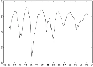
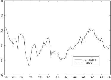
to long run shocks. In figure 2 we compare the implied utilization rates (calculated as

[1+

exp ( tjT

)] 1

), with those calculated by the FED, according to the procedure

outlined above.

The comparison reveals that the profile of the two measures is pretty much the

same, although the FED estimates are somewhat slightly trending downwards, whereas

our estimates hover around a constant level. The main message conveyed by the plot is

that the univariate model, despite its simplicity and the little information requirements,

does a good job in replicating the dynamics of the utilisation rates.

When we treat

as an unknown parameter, the estimated variances of the

distur-bances to both components are somewhat larger. Since the ML estimate of

is less than

the value imposed for the previous model (

^

=

:

06), and corresponds to an average

util-isation rate of 0.94, the capacity series gets closer to the production index (see figure 3);

further, its dynamics are somewhat rougher.

Estimates of the utilization rates, displayed in figure 4, reproduce the dynamics of

figure 2, in the sense that the alternation of low and high capacity utilization regimes

coincides with that highlighted by the FED estimates. However, they oscillate around a

trade-off between the smoothness of capacity and of the utilization rates; usually it is believed

that capacity should be slowly changing, whereas the utilization rates, which are affected

by short run variations, ought to be more volatile.

As far as the average level of capacity utilization is concerned, is a well known fact

that “data based” utilization rates tend to be systematically higher on average than those

computed employing survey based data (Christiano, 1981). This simple example conveys

the message that the main uncertainty concerning capacity measurement concerns the the

average level of capacity, rather than its dynamics.

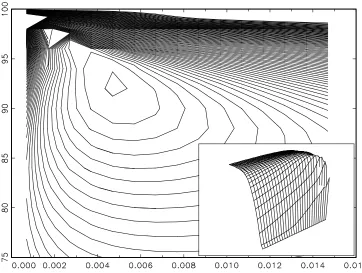
Likelihood contours for the problem at hand, considered as a function of and the

innovation ratio 2 !

= 2

are plotted in figure 5. The cycle parameters were fixed at=:98

and c

= :11. The picture shows on the y axis the utilization rate, (1+) 1

, and the

innovation ratios 2 !

= 2

on the horizontal axis, and confirms that the likelihood is well

behaved, although relatively flat going in the top-left bottom-right direction: in general,

for lower average utilisation rates we expect smoother capacity estimates and rougher

utilization rates.

4

The Bivariate Model

In some countries direct measures of capacity utilization are elicited by business surveys,

asking a sample of companies the percentage at which the company operates in the

ref-erence period. In Italy, for instance, a judgmental survey is conducted quarterly by ISCO

(Istituto Nazionale per lo Studio della Congiuntura) for the manifacturing sector. The

in-dividual responses are then aggregated with weights proportional to a measure of size of

the firm, such as value-added or the number of employees. The respondent is offered no

formal definition, apart from a generic reference to maximum capacity as an upper limit.

The resulting estimates are affected by both sampling errors and non sampling

units usually leads to a gross underrepresentation of small productive units. We shall not

deal with this source of systematic error in the sequel, firstly because it is not easily

quan-tified, secondly because the output measure, at least in Italy, suffers from the same sample

selection bias.

Furthermore, there are two main sources of ambiguity that harm the interpretation

of the results; the first arises as a consequence of the fact that the definition of capacity

is left to the respondent, who may alternatively refer to either a particular productive

factor, namely capital, or to all resources. The second element is “the time horizon that

businesses have in mind in evaluating their capacity” (Christiano, 1981, p.171).

Nevertheless, these measures cohere with the information coming from other sources

and display dynamics reflecting the stage of the business cycle, and what is more, they

can make a significant contribution to the information set for estimating capacity. In this

section we shall make an attempt to incorporate this additional information into a suitable

multivariate structural time series model.

LetU

t denote a survey based measure of capacity utilization, taking values within

the range (0,1] andu

titslogittransformation, namely:

u t =ln U t 1 U t :

We are now in a position to introduce the following bivariate model:

y t

= t

ln[1+exp ( t

)]+" 1t

u t

= b+ t

+" 2t

:

(6)

The second equation captures the idea that the survey based measure has extra

vari-ability due to a measurement error. Since the data sources are independent, it is quite

natural to assume that the measurement noises " 1t and

"

2t are mutually and serially

un-correlated. It should also be noticed that t enters both equations: as a matter of fact, it

is the latent factor of the logit transformation ofU

enters non linearly in the equation fory

t, being the source of the short run fluctuations in

the utilization rates.

Whereas in the univariate case we assumed the stationarity of t, the increase in the

information set can allow more precise statements on the time series properties of the data

generating process for the utilization rate. More precisely, a particular specification for it

may be suggested by the univariate analysis ofu

t. Finally, the parameter

=exp ( b)can

be concentrated out of the likelihood function and estimated in terms of^ b=N

1 P

u t.

As far as the statistical treatment is concerned, the only source of non linearity is the

first measurement equation; the model can be linearised by a first order Taylor expansion

as was done in section 2. The resulting approximated model is conditionally gaussian and

likelihood evaluation and prediction can be performed by means of the extended Kalman

filter with diffuse initial conditions.

As a further extension, it would be interesting to explore the possibility to employ

the information arising from capital stock estimates, which are built in some countries

ac-cording to the perpetual inventory method. Following the point (ii) of the FED procedure,

one can suitably assume that capacity and capital stock are cointegrated with

cointegrat-ing vector [1 1]. This enhances the smoothness of the capacity estimates since the

perpetual inventory methodper seresults in a one sided MA filter applied to the

invest-ment series, smoothing out the high frequency components (although inducing a phase

shift). The model (6) would be amended so as to contain a common trend which enters

log-capacity and the capital stock equation with loadings matrix[11] 0

5

Illustration: Capacity Estimates for the Italian

Indus-trial Sector

In this section we derive capacity estimates for the Italian industrial sector, by applying

the model (6) to a bivariate system made up of the index of industrial production (IP) and

the index of capacity utilisation produced by ISCO. The former is available on a monthly

basis and we consider the seasonally adjusted series with trading days correction. The

latter is available only quarterly, and the most straightforward solution is to aggregate the

IP series to the same observation interval.

Time aggregation is an issue, since for the ISCO series there exists some uncertainty

surrounding the time horizon considered by the respondent in practice; in particular, it is

unclear whether reference is made to the end of the quarter or to the average capacity

utilization over the quarter; the survey question is formulated in terms of the latter, asking

for an assessment “in the course of the quarter”. On the contrary, the entire questionnaire

makes explicit reference to the situation at the end of the quarter; moreover, the respondent

is more likely to refer to the end of period situation in the capacity assessment.

Therefore, we assumed that the quarterly utilization rates are end of period estimates

and we derived a quarterly production series taking a systematic sample of the series

values referring to the last month of each quarter (March, June, September, December).

The sample period goes from the first quarter of 1970 to the fourth quarter of 1993.

Univariate structural time series modelling ofu

tsuggested a stationary AR(1) plus

noise specification for t; table 2 reproduces the maximum likelihood estimates obtained

via the diffuse Kalman filter for the unrestricted case and when the smoothness prior,

2 !

=0, is imposed.

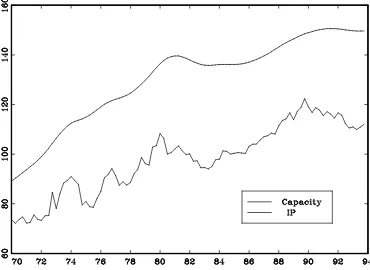
Figure 6 shows the smoothed estimates of capacity,exp ( tjT

), obtained from the

re-stricted model, which, although is not the preferred model, according to the information

high-lights that at the beginning of the 80’s a slowdown affected capacity growth. In figure 7

the implied capacity utilization rates,[1+ ^ exp (

tjT )]

1

, are compared with the ISCO

series, showing that the noise in the latter is somewhat smoothed out.

6

Interpolation

Usually, since the output series are monthly, it is desirable to estimate capacity with the

same periodicity. This need justifies the interpolation technique adopted by the FED

and the peak to peak interpolation in the Wharton Index methodology. The techniques

adopted are quite elementary and result in linear interpolation. The interpolation problem

can actually be solved within the models we have proposed in the previous sections, by a

suitable modification of the measurement equation.

We thus turn our attention to the problem of estimating the model (6) using the

monthly index of production and the quarterly utilization rate series. The latter is subject

to missing values in a systematic fashion, since the first and the second month of each

quarter are not observed. As the unobserved components are stock variables, time

disag-gregation is less of a problem and the model (6) holds at the monthly level without any

modification.

A possible strategy is illustrated in De Jong (1991b), and amounts to setting the

missing values to zero and zeroing out the elements of the measurement equation system

matrices corresponding to the series. This produces a singularity in the covariance

ma-trix of the Kalman filter innovations, which is remedied upon replacing its inverse by a

generalised inverse, using a selection matrix picking up a suitable basis for this matrix.

Preserving the AR(1) specification for t, the maximum likelihood estimates of the

hyperparameters in the unrestricted case are as follows (lnL =1355:76):

t

=0:96 t 1

+ t

; t

^ 2 !

=53710 7

; ^ 2

=:410 7

; ^ 2 " 1

=216910 7

; ^ 2 " 2

=555510 7

.

When the smoothness prior is imposed on the model for capacity, the

hyperpa-rameter estimates are the following (lnL = 1349:66): ^ 2

= 13 10 7 ; ^ 2 " 1 =

248810 7

; ^ 2 " 2

=703910 7

. The model for tis unchanged:

t =0:96 t 1 + t ; t

WN(0;:00182);

The smoothed estimates of productive capacity obtained from the second model

are graphed in figure 8. The series reproduces the behaviour of capacity observed at a

quarterly reference period with the monthly variability being absorbed by the utilization

rate, reported in figure 9.

7

Conclusions

In this paper univariate and bivariate models for measuring capacity and its utilization

were introduced, that are consistent with the recent developments of the econometric

analysis of time series. They are nonlinear structural time series models that estimate

capacity as the saturation level of output.

The performance of the models was illustrated with respect to the US and the Italian

industrial production, and our conclusion is that they qualify as an useful addition to

the currently available methods. Not only do they provide a rationalisation of the ad

hoc procedures used by statistical agencies, but they also allow important issues such as

interpolation to be treated within the same model based framework.

Furthermore, suitable extensions can be envisaged that can deal with related

mea-surement issues, arising when a series is subject to an upper or lower bound, e.g. in the

extraction of the natural rate of unemployment, and so forth.

Financial support from MURST, Funds ex-60%, is gratefully acknowledged. I am

REFERENCES

Christiano L.J. (1981), “A Survey of Measures of Capacity Utilization”,IMF Staff Papers,

28, 1, 144-198.

DeJong P. (1991a), “The Diffuse Kalman Filter”,Annals of Statistics, 19, 2, 1073-1083.

DeJong P. (1991b), “Stable Algorithms for the State Space Model”,Journal of Time Series

Analysis, 12, 2, 143-157.

DeSerres A., Guay A., and St.Amant, P. (1995), “Estimating and Projecting Potential

Output using Structural VAR Methodology: The Case of the Mexican Economy”,

MimeoBank of Canada.

Evans, G.E. (1989), “Output and Unemployment Dynamics in the United States: 1950:1985”,

Journal of Applied Econometrics, 4, 213-237.

Granger, C.W.J. (1991), “Some Recent Generalizations of Cointegration and the Analysis

of Long-Run Relationships”, in Engle, R.F. and Granger, C.W.J. (eds.) Long-Run

Economic Relationships. Readings in Cointegration, Advanced Texts in

Economet-rics, Oxford University Press, 277-287.

Harvey A.C. (1989), Forecasting, Structural Time Series Models and the Kalman Filter,

Cambridge University Press, Cambridge, UK.

Kuttner K.N. (1994), “Estimating Potential Output as a Latent Variable”,Journal of

Busi-ness and Economic Statistics, 12, 3, 361-368.

Raddock R.D. (1985), “Revised Federal Reserve Rates of Capacity Utilization”, Federal

Sargent T.J., and Sims C.A. (1977), “Business Cycle Modeling without Pretending to Have

Too Much A Priori Economic Theory”, in Mew Methods in Business Cycle

Re-search(C. A. Sims, ed), Minneapolis, Federal Reserve Bank.

Wallis, K.F. (1987), “Time Series Analysis of Bounded Economic Variables”, Journal of

Table 1:US Industrial Production, 1967:1.1996.6. Parameter estimates, Diagnostics and Goodness of Fit.

=1

=m

1

unrestricted ^

2

0 0

^

2

! 83 256

^

2 11952 56113 ^

.98 .99 ^

c .11 .11

^

.06

lnL 1683.96 1686.94

AIC -3361.92 -3363.88 BIC -3342.41 -3346.37

R

2

d .13 .11

r

1 .23 .24

Q

(12) 39.93 48.65

G

1 2.67 0.56

G

2 64.23 43.19

G

66.90 43.75 NOTES: All variances are multiplied by10

7

. r

1 denotes the residual correlation at lag 1.

Q(12)is

Ljung-Box statistic based on 12 residual autocorrelations. G

1 is a test for residual skewness based on

the standardised third moment of the residuals about the mean (see Harvey, 1989, 5.4.2.); G

2 is a test

for residual kurtosis andG = G 1

+G

2is the Bowman and Shenton test for non-normality. R

2 D

=1 SSE=SSD, whereSSEis the residual sum of squares andSSDis the sum of squares of the centered first

differences. The Akaike Information Criterion is computed as AIC= 2lnL+2h, wherehis the number

[image:21.595.227.383.133.347.2]

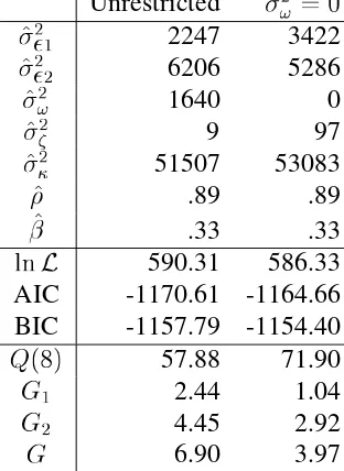
Table 2:Italy, Bivariate Model for Capacity Estimation, 1970:1.1993.4. Unrestricted 2 ! =0 ^ 2 1 2247 3422 ^ 2 2 6206 5286 ^ 2

! 1640 0

^ 2 9 97 ^ 2 51507 53083 ^ .89 .89 ^ .33 .33

lnL 590.31 586.33

AIC -1170.61 -1164.66 BIC -1157.79 -1154.40

Q(8) 57.88 71.90 G

1 2.44 1.04

G

2 4.45 2.92

G 6.90 3.97

NOTES: see notes at table 1. The statisticsQ(8);G 1

;G 2 and

Gare the multivariate Ljung-Box and

[image:22.595.144.515.294.568.2]

Figure 1: US Capacity,exp (

tjT

), and Industrial Production. The parameter

is set equal

[image:23.595.143.515.288.563.2]

Figure 2: US Index of Capacity Utilisation. The parameter

is set equal to (1

=m

1),

[image:24.595.142.515.294.566.2]

Figure 3: US Capacity (upper line),exp ( tjT

), and Industrial Production (lower line). The

[image:25.595.143.516.291.559.2]

[image:26.595.145.507.300.573.2]

Figure 5: Likelihood Contours. The vertical axis measures the utilization rate,(1+) 1

, and the horizontal axis the ratio

2 !

= 2

[image:27.595.145.515.296.566.2]

[image:28.595.142.515.289.559.2]

[image:29.595.146.513.287.561.2]

[image:30.595.143.515.290.558.2]