Using Discrete Wavelet analysis and Sequential test to
detect the endpoint in CMP process
Sihem Ben Zakour Hassen Taleb
Department of quantitative methods Department of quantitative methods
Higher institute of management of Tunis,Tunisia Higher institute of Business administration of Gafsa, Tunisia
ABSTRACT
Due to the development in new technologies like semiconductor industry, with advances in sensors and information technology oblige us to handle with large datasets do not stop increasing, while monitoring devices are becoming more and more complexes and sophisticated. As the measurement points become closer. Among the complex monitoring process, the detection of the end of polishing (EPD) during the chemical mechanical planarization (CMP) process is considered as a critical task in semiconductor manufacturing. In this paper, an Acoustic emission (AE) signal is collected during the progression of the CMP process will be monitored using an online method in which the signal will be preprocessed using wavelet analysis (WA) to clean the data from noise and at the same time, a sequential probability ratio test (SPRT) will be developed. This test was applied to the wavelet decomposed. Eventually, it has shown to be efficient in controlling complex processes and suitable for real-time application by developing a moving block strategy.
General Terms
Wavelet Representations Signal Processing, Adaptive Control, Sequential Decision Theory.
Keywords
Sequential Probability Ratio Test (SPRT), End point detection (EPD), Chemical mechanical planarization (CMP), Acoustic emission (AE), Wavelet Analysis (WA), monitoring process.
1.
INTRODUCTION
The semiconductor wafer, composed by a tranche of silicon on which one comes to deposit successive layers of metallization, has been a subject of interest these last years. Indeed, the reduction of its size, the introduction of new materials like the copper and low-k dielectrics and the superposition of different metals create an enormous challenge in terms of accomplishment of wafer production and checking its quality. The CMP process combines mechanical and chemical properties. Hence, the chemical agents react to the surface of wafer and transform it. The abrasive particles come to remove this layer of transformed matter. Joseph et al. [1] define three main players in this process, shown in figure 1, presented by: 1. The surface to be polished. 2. The pad - it is called fabric and has a porous structure which enables it to transport the slurries towards the
[image:1.595.319.563.280.432.2]wafer, and thus facilitates the chemical action 3. The slurry provides both chemical and mechanical reactions.
Fig 1: Chemical mechanical planarization (CMP) machine
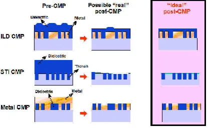
During the polishing, it seems necessary, even crucial to determine the right moment of stopping this process, as shown in figure 2.
Fig 2: The need of CMP process to achieve ideal planarization
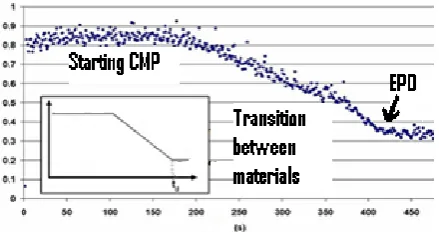
[image:1.595.320.528.497.630.2]non-stationary of CMP seems to be a necessity. Due to the difference between materials, AE sensor is implemented to monitor the process and to detect transitions from one layer to another, during the progression CMP, shown in figure 3.
Fig 3: Evolution of an acoustic signal during the polishing
In this paper, Sequential Probability Ratio Test (SPRT) for variance and coefficient of variation applied on the wavelet decomposed AE data will be presented. A comparaison between these two tests will be conducted to identify the most powerful one. The organization of this paper is as follow: An overview of wavelet based multi-resolution analysis will be present in section 2. In section 3, detailed description about the online monitoring using SPRT will be proposed. The experimental setup and results will be given in section 4. In section 5, presents the concluding remarks and future researches.
2.
OVERVIEW OF WAVELET BASED
MULTIRESOLUTION ANALYSIS
In general, statistical analysis picks out a sample with the aim of making inferences about the population from which the sample is selected. But last years, the need to increase the number of fields has become more widespread and offers more efficiency. The real-life data observed, taken from the sample, are called functional data (FD) [6] which incorporate rich information about process conditions. The representation of process as a signal can include different phenomena such as mean shift, variance shift and noise. Hence, they do not have stable probability distribution. Monitoring FD in such process is to analyze process variables at multiple locations and the precision in time-frequency localization is achieved made thanks to the use of wavelet based multi-resolution analysis (MRA) approach. Modelling time-series has appeared as an interesting approach to explore the dynamics process. Classical time-series methods can only be used for stationary time-series (in which the density probability distribution and properties do not vary with time). However, monitoring polishing time-series are typically noisy, complex and strongly non-stationary. Given this specific nature of the signal, wavelet analysis appears particularly attractive because it is well suited to the analysis of non-stationary signals. Recently, a lot of papers use wavelet analysis in many applications, we can mention some of them in Politic [7], time series analysis [8], medicine [9], Geophysical [10], also in semiconductor industry [11]. Here, we will give a review about multi-resolution analysis and wavelet analysis.
2.1
Multi-resolution analyses
Mallat [12] is the pioneer of MRA. This method allows to represent data at different levels of resolution and to study the data features situated at a specific and the desired scale. The main component is the vector spaces. For each vector space, there is a vector space of higher resolution until getting the highest possible resolution. Mallat’s transform
J
subspaces
V
0
V
1
V
2
....
V
j (1) The MRA follows the following conditions:
V
j
V
j1,
j
Z
(2) Where, Z denotes the set of all integers.2
( )
j j
V
V
L R
j 1W
(3)
{0}
j j
V
V
(4)For
f x
( )
L R
2( )
1
( )
j(2 )
jf x
V
f
x
V
(5)
( )
j(
)
jf x
V
f x k
V
(6)
Which represent respectively the scale and the shift invariances. Another method is used to obtain V J by eliminating the orthogonal complement from the higher space VJ+1. Thus, the orthogonal complement space W j is defined as follows:
W
j
{
f
V
j1f g
,
0,
g
V
j}
(7) Where <o,o> represents an inner product of linear functions. The space W j fills the difference between VJ+1 and V J ( Vj+1= Vj
W j ), with
the orthogonal summation. Hence, VJ can be represented by the nested orthogonal summation1 2 1 0 0
...
j j j
V
W
W
W
W
V
(8)( )
t
is a Mother wavelet, used to define details for each fixed j which will be2
2
,
( )
2
(2
)
j
j
j k
t
t
k
j k
,
Z
(9)With
( )
t
0.
And scaling function called also a Father Wavelet,
2
2
,
2
(2
)
j
j
j k
t
k
(10)With
( )
t
1.
examine global characteristics at a zoomed-out level by focusing in on low frequency components and also examine local behavior at a zoomed-in level by analyzing high frequency components at a particular location along the x-axis. The benefits of MRA for statistical process control (SPC) are the detection a wide range of process changes, also the identification of the type of change and its location along the x-axis. For more details concerning MRA see [14].
2.2 Wavelet analysis
2.2. 1. From Fourier transform to wavelet
transform
Fourier Transform (FT) is a tool for analysis and processing of many natural signals. It is a function which converts the signal from time versus amplitude to frequency versus amplitude. In spite of offering the possibility to detect many of these periodicities, it cannot determine temporal variations. That is why, all the temporal information in the signal are lost. It is a purely frequency localization domain. Another shortcoming appears due to the assumption of signal in FT which obliges us to use specifically of a periodic and stationary signal. To solve this problem, the Short-Time Fourier Transform (STFT) or Windowed Fourier Transform (WFT) has the ability to convert the signal to frequency versus time and gives information about signal simultaneously in the time domain and in the frequency domain. The capture of the temporal aspects is done by analyzing a short segment of the signal at a time through the use of a fixed window size. STFT has not the ability to get a decent resolution for both high and low frequencies. This dilemma of resolution is explained as follows: having narrow window corresponds to poor frequency resolution and having wide window corresponds to poor time resolution. Hence, a new time-scale based Wavelet Transform (WT) has appeared. The first one that developed this technique is Calderon in pure mathematics [15]. It is a kind of extension of Fourier analysis. It shows its power as mathematical tool for analyzing stationary and non-stationary signals and providing excellent time-frequency localized information due to the presence of several aspect ratios. To get more accuracy in low-frequency information, the use long time intervals will be necessary, and for high-frequency information, the shorter regions will be required. Hence, High frequency components capture the least smooth function behaviour while low frequency components capture smooth features. In wavelet analysis (Time-Frequency domain), some frequency localization and some time localization are maintained, so it is a compromise between using filters (time domain) and Fourier transforms (frequency domain). Wavelet analysis can model complicated functions with sharp changes and discontinuous derivatives, computationally efficient, useful for online applications, and signal identification in presence of noise, able to de-correlate auto-correlated observations, adaptable to the changing scale of the function offering a good frequency and time resolution.
[image:3.595.315.534.75.197.2]
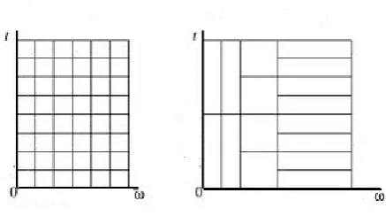
Fig 4: On the left Window Fourier transform and on the right Wavelet transform
As we see in figure 4, for time–frequency resolution of the wavelet approach, when the scale decreases, the time resolution improves but the frequency resolution gets poorer and is shifted towards high frequencies. Conversely, an increases the boxes shift towards the region of low frequencies, the height of the boxes becomes shorter (with a better frequency resolution) but their widths are longer (with a poor time resolution). In contrast with wavelets, all the boxes of the windowed Fourier transform are obtained by a time- or frequency shift of a unique function, which yields the same variance, spreads over the entire time–frequency plane. With wavelet transform of a signal is defined
* *
,
1
( , )
( )
(
)
( )
( )
x a
t
W a
x t
dt
x t
t dt
a
a
(11)2.2. 2 De-noising procedure
The wavelet analysis uses linear combinations of basic functions (wavelets), localized both in time and frequency, to represent any function in the L2(R) space. It provides a tool for time-frequency localization.
, ,
( )
j k j k( )
f t
b w
t
(12)Where j is the dilation (or scale) index and k is translation index. Wj,kdenotes a collection of basic functions, and bj,k
designates the coefficients of these functions. Also the wavelet basis functions can be derived from the dilation and
translation of scaling functions
( )
that span the subspace L2(R). By the combination of the scaling and the wavelet functions, any class of signal will be represented as follows:0
0
, ,
( )
j k(
)
j k(2
j)
k k j j
f t
c
t k
d w
t k
(13)Where
c
jo,k andd
j,kare coefficients for the scaling andwavelet functions, respectively. They are also called the discrete wavelet transform (DWT) of the function and it is customary to start with j0=0. If the wavelet system is
0,,
( ),
0,( )
( )
0,( )
j k j k j k
c
f t
t
f t
t dt
(14),
( ),
,( )
( )
,( )
j k j k j k
d
f t w
t
f t w
t dt
(15)The de-noising objective is to suppress the noise part of the signal S and to recover f.
S
f
noise
(16)2. 2. 2. 1 Decomposition
The first step in this procedure is decomposition: at this stage, the appropriate wavelet is selected according to its associated properties given by the table 1.
Table1. Summary of wavelet families and associated properties
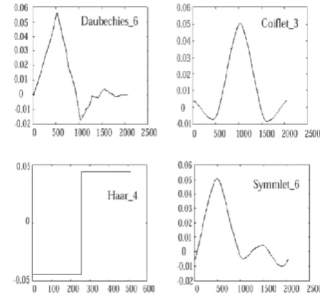
Hence, making the choice of a wavelet could be made according to these type classifications continuous versus discrete wavelets, orthogonal versus redundant decompositions. Briefly, the continuous wavelets present a disadvantage concerning redundancy in decomposition, but they are more robust to noise compared with other decomposition schemes. Discrete wavelets have fast implementation but generally, the number of scales and the time invariant property depends closely on the data length. In figure 5, different types of wavelet have presented. The differences between different mother wavelet functions (e.g. Haar, Daubechies, Coiflets, Symlet and etc.) show the manner of these scaling signals and the wavelets are defined.
Fig 5: Different families of wavelet
It should be noted that the number near to wavelet type correspond to the vanishing moment – 1 (n = N − 1). Also, Haar wavelet has the same representation of Daubechie 1. All wavelets are indexed by the number of vanishing moments.
There are several methods for choosing the higher level of decomposition , among them we can cited, after
decomposing the signal of length (n) to the maximum allowed level of decomposition j=n/2,
1) Apply threshold value and observing the significant coefficients
2) Calculate the Energy function and choose the level after which there is a significant drop in the energy content
2 2
, 1
( )
(2
)
n
j
j j j k
k
EN
f t dt
d w
t k
(17)3) Making test to the noise at each level of decomposition and stopping the test when the noise is removed
4) Define the denoising level and use an iterative scheme in which the relative difference of the energy is consider as a stopping criterion.
Finally, Calculating the coefficients
0,
j k
c
andd
j k, from the scaling and wavelet functions, respectively as showen in figure 6.Property Haar Db Sym Coif
Crude
Infinitely regular
Arbitrary regularity * * *
Compact supporte orthogonal
* * * *
Compact supporte bi-orthogonal
Symmetry *
Asymmetry *
Near symmetry * *
Arbitrary number of vanishing moment
* * *
Vanishing moment for father wavelet
*
Existence of father wavelet
* * * *
Orthogonal analysis * * * *
Bi-orthogonal analysis
* * * *
Exact reconstruction * * * *
FIR filters * * *
Continuous transform * * * *
Discrete transform * * * *
Fast algorithm * * * *
[image:4.595.314.539.247.457.2]Fig 6. A diagram showing analysis of cj — 1 into cj and dj. Approximation coefficients and detail coefficients at scale j can be obtained from approximate coefficients at scale j–1.
2.2.2.2 Thresholding
The second step of de-noising procedure is thresholding in which the thresholded value is calculated using Visushrink method (or Donohos universal threshold rule proposed by Donoho et al.[ 16, 17]and is given as follows:
2 log( )
j j
t
n
(18)Where n: the length of signal and
j is the standard deviation of the noise at scale j.,
1
(
)
0.675
j
median d
j k
(19)Where
d
j k, are the wavelet coefficients. The
j is the standard deviation (j) estimated from the median of the absolute deviation of the wavelet coefficients at the same scale j. Only the significant wavelet coefficients situated outside of the threshold limits are extracted by applying soft or hard thresholding. The thresholded coefficients are given as follow:1) Hard thresholding:
, ,
, ,
0
j k j kj k j k
if d
t
d
d if d
t
(20)
2) Soft thresholding:
, ,
, , ,
0
(
)(
1)
j kj k
j k j k j k
if d
t
d
sign d
d
if d
t
(21)Where sign (dj ,k ) is the positive or negative sign of the
wavelet coefficient dj ,k. For more details about soft and hard
thresholding read [16, 17, 18, and 19].
2.2.2.3 Reconstruction
The last step of wavelet analysis is reconstruction. The signal ft is reconstructed from the thresholded wavelet coefficients through the use of inverse wavelet transforms. After the determination of the thresholded details and approximations at level J, they will be used as inputs to calculate the coefficients at level (j-1) until getting the original signal with the noise eliminated. The reconstructed signal at the level j is as follows:
,
( )
(2
j)
j j k
k
f t
d
w
t
k
(22)
3
. ONLINE MONITORING STRATEGY
USING SPRT AND WA
3.1 SPRT
Wald [20] defined a parametric statistical test, named sequential test, where the number of data collected is not predetermined and treated as a random variable. This method is developed especially for monitoring the quality of a specific product. The sequential method of testing a hypothesis H has three decisions at any stage of experiment: (1) To accept the hypothesis H0. (2) To reject
the hypothesis H0. (3) To continue the experiment by
making an additional observation. In classical hypothesis testing, analysis and conclusion are done until all the data are collected and the size of samples is fixed. In contrast, Wald’s sequential probability ratio test is different from the above test; every sample collected is analyzed immediately in a sequential manner. And, to construct the most powerful test for simple test, the Neyman- Pearson (N-P) Lemma , states that, for a fixed sample size of (n), the optimal design (the most powerful test) for simple hypothesis (H0 against H1) can be obtained from the likelihood ratio (
n ) is given by:Accept H0 if
n
k
(23)
Reject H0 if
n
k
(24)With 1
1 0
(
)
(
)
ni n
i i
f X
f X
(25)k is the decision limit associated with level of significance
(the critical region size), and (i) denotes the observation index. The distribution of Xi must be Gaussian for implementing SPRT because this test is not applied to the original data but to the wavelet details (which is the Xi). Applying SPRT on the variance and CV of wavelet details, the upper control limits are needed to detect the end point.The parameters of SPRT chart are
0,
1,
and
.
And, the equations A,
0and
1are defined as follow:2 1
2 0
2 2
0 1
1
2 log(
)
log(
)
1
1
(
)
n
A
n
(25)
2 4
0 0
4
( 1
)
*
c
S
h
S
c
2 4
1 1
4
( 1
)
*
c
S
h
S
c
(27)The values of h0 and h1 are selected according to the
datasets and
c
4 is a constant and depend only on the valueof n, expressed by:
4
4(
1)
(4
3)
n
c
n
(28)In table 2, SPRT for variance and SPRT for coefficient of variation are presented. H0 is verified for the variance if its value exceed A and for coefficient of variation if the
[image:6.595.58.292.324.447.2]coefficient exceed
A
/
ATable 2: SPRT for variance and coefficient of variation
3.2. Real time multiscale monitoring
methodology
An online methodology with multiscale analysis to monitor the status of the wafer polishing. It contains two stages: Firstly, the application of wavelet based multiresolution analysis in online strategy. Secondly, using the data analyzed previously to control the progression of CMP process keeping it in the real time implementation [21]. The implementation of sensors allows to measure and to convert the output of data and the environmental factors into signal. Subsequently, to transmit the obtained signal to data acquisition system. The PC based DAQ system is charged of the acquisition of electrical signals and digitized it. To make interface between data acquisition system (DAS) and MATLAB, the use of appropriate scientific engineering software will be unavoidable allowing the transfer of the data digitized by DAS at a particular dyadic length, to a (.m) file in MATLAB. The obtained Matlab file is considered like the first block of input. This latter is executed automatically to analyze digitized data. The execution of multi-resolution analysis will be as follow: Firstly, the decomposition, in this step, selecting the depth of wavelet decomposition to optimize the representation of the filtered signal. We select also the dyadic width of the testing window which should not less than the high level of decomposition, the choice of
wavelet type is done according to the type of the studied data. Secondly, thresholding only the details with the appropriate thresholded values to obtain only the coefficients which have significant information about the monitored process. After that, reconstruct the signal from the thresholded wavelet coefficients. This signal will be studied using an appropriate statistical test. The choice of the test should take into account the integration of online implantation to make good decision about the quality of the product. The application of statistical testing is done to the details obtained from wavelet reconstruction. Hence, the control chart should not only being adaptable to the online implantation but also very sensitive to small change in the signal due to the use of details usually very small in magnitude and any change in these details caused by an assignable event is smaller. The real-time implementation does not specify the moment of stopping the process and therefore it does not precise the length of data previously. Given the reasons mentioned above, the use of sequential probability ratio test will be considered as the perfect choice in this case. The real-time methodology has the ability to display real-time SPRT plots and to detect the event of interest when it occurs. The strategy of moving block is computationally able to deal with very high data collection rates by writing an efficient code that does not require storing of huge data in the temporary memory of the computer. The details were plotted and SPRT chart defines the hypothesis test. When H0 is rejected, the wavelet details
and SPRT chart are plotted only till this moment.
3.3. Online moving block strategy in SPRT
The first dyadic data block is formed, through the use of data acquisition systems. The data are wavelet decomposed into coefficients at the appropriate level based on data type. After that, the obtained coefficients are denoised using thresholding methods and reconstructed into the time domain. Standard deviation of the wavelet details in the first data block is calculated and affected to
s
. The value ofs
will be used to calculate
0 and also
1. The mean also should be countedin order to determine the coefficient of variation. Hence, the two SPRT limits are specified. At each block containing the new collected data to be monitored, the variance and coefficient of variation of wavelet detail are defined and plotted against the SPRT limits. The standard deviation of each point in new block is equal to the standard deviation of all the previous wavelet details until the current point. At each new formation of data block, one must always up-date the standard deviation and coefficient of variation of the wavelet details. The value of
s
will be equal to the average of the standard deviations of the current and all of the past blocks. And the values of
0 and also
1 will change according tothe new value of
s
. Hence, the upper SPRT limit of CV and variance are also up dated. As, the upper control limit for every block are drawn from the data itself, allow us to have robust limits against all the fluctuations in the details. The desired event occurs (correspond on the acceptance of H1), when the increased value of the variance of the wavelet details exceed the upper control limit of the SPRT chart. And, exceeding the upper limit of the control chart will indicate the beginning of the end of planarization. The sequential test will be programmed using Matlab.For variance
For CV
Reject HO
2
n
A
n/
n
A
/
AKeep on sampling
2
n
A
4.
DESCRIPTION OF EXPERIMENTAL
SETUP AND RESULTS
[image:7.595.318.542.72.231.2]The test bad should be equipped with an AE sensor in order to collect the data during CMP. The raw signal is non stationary since the mean value change during the progression of CMP process. The planarization of the wafer is done under a specific combination of rotational speed (rpm) and downward pressure (psi). In this paper, the studied data are simulated. A sample of these data, plotted in figure 7, shows the presence of noise which should be eliminated to have a robust statistical tool used in monitoring the CMP process.
Fig 7: The representation of the simulated raw acoustical signal
The amplitude of the AE signal tends to decrease during the progression of polishing procedure allowing to better situate the status of wafer (under polished, desired level of polishing, over polished). The non-stationary mentioned above, the presence of white noise and the autocorrelation in AE signal have justify the use of wavelet analysis. The examination of the AE signal in offline method is done after collecting the entire signal (after CMP process was completed) makes the right moment of stopping the polishing process at the right moment is redoubtable. Furthermore, the application of dyadic discretization (wavelet decomposition with down sampling by two) in offline implementation, is made by the choice of the longest possible Dyadic length (correspond to the entire data length) from the prescreened data but it can introduce time delay in the computation of the coefficients at no dyadic locations, which will be very apparent at coarser scales. To surmount these two problems, the need of an online approach was perceived. The strategy ofdetecting the occurrence of the desired event employs specific segments of the data generated during the progression of the CMP process called moving block. When the CMP progresses and the collected data length is equal to the selected window width, the analysis begins. The first step of the denoising procedure is done for the data in the
first block.
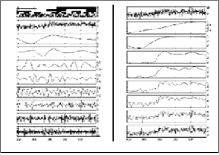
Fig 8: The Multi-resolution of the simulated signal
(on the left coefficients signal and details, on the right signal and approximations)
In figure 8, at each scale of decomposition, the high frequency
is filtered out, represented by the detail coefficients
.
Secondly, the application of soft thresholding to the resulting wavelet coefficients at each scale of decomposition. The reconstruction of details in time domain is done from the thresholded wavelet coefficients. At each new formed window, all details are checked. The values of
and
are equal to 0.1 and 0.1 respectively. And the choice of the values h0and h1 equal to 2and 1.5 are made according to the simulated data, in order to optimize the power of SPRT chart. The wavelet chosen is Daubechies fourth-order wavelet basis functions (db4) since it is more widespread and practical in the discrete wavelet analysis. The highest energy value, which corresponds on the depth of decomposition, is equal to 8. Hence, the dyadic block width should be equal to 8 (contains 256) as the minimum length value. And the multi-resolution analysis is restricted to eight levels of decomposition. At each scale of decomposition, the high frequency filtered out shows by the detail coefficient. Theoriginal signal will be approximated through the use of the set of the basic functions (wavelets) of the first scale in order to give the approximation coefficient a1 and the coefficient
detail d1 represents the difference between the first approximation signal a1 and the original signal. To determinate
approximation at level two, a1 is taken and approximated by a
set of basis of the second scale to obtain a2 with d2 the
difference between a1 and a2. The same work is done until the
[image:7.595.55.292.217.320.2]Deviation is a measure of how closely a series of numbers tracks from its expected value and the coefficient of variation measures the spread of a set of data as a proportion of its mean. Based on this simulation, the acceptance of H1 is verified on the 231 point for variance SPRT and 202 collected point for the coefficient of variation. The SPRT for the first block are plotted. The SPRT of variance plotted against its upper limit in the first dyadic block. It is useless to form a new block. As the normal distribution have two parameters: mean and variance, employing coefficient of variation seems to be more reliable and efficient for detecting the end of polishing.
5. CONCLUSION AND FUTURE WORK
The most industrial processes are represented by data situated at multiple scales due to the occurrence of various events in a process at different time and frequency localizations. Hence, the application of wavelet analysis in the context of system identification has become ineluctable. And the best strategy for monitoring the wafer in the semiconductor industry is the online strategy based on Acoustic emission sensors. This strategy is widespread due to drawbacks of the offline method. In this paper, the acoustic signal has been analyzed using wavelet based multi-resolution. At the same time, each constructed block will be monitored using SPRT for variance and CV. This SPRT chart is applied to the reconstructed details coefficients to detect the end point, showing its performance in detecting the end point. But, CV SPRT allows detecting the starting of the end point of polishing earlier compared to variance SPRT. This result is expected due to the use of pre-proceeded detail coefficients, by wavelet analysis, which follows normal distribution. The suggested researches in the future are examination of the on-line performances using wavelet-based multi-scale to different defect in CMP process, using wavelet analysis to identify the type of defect according to the obtained values of decomposed coefficients (studying local changes using wavelet analysis to differentiate the type of defects).
6. REFERENCES
[1] Joseph M. Steigerwald, Sgyam P. Murarka and Ronald J. Gutma, 1997, Chemical Mechanical Planarization of Microelectronic.
[2] P. B. Zantye, A. Kumar, and A. K. Sikder, 2004, Chemical mechanical planarization for microelectronics applications, Mater. Sci. Eng. R. Rep., vol. 45, nos. 3–6, pp. 89–220.
[3]W. Lih, S. T. S. Bukkapatnam, P. Rao, N. Chandrasekaran, and R. Komanduri, 2008, Adaptive neuro-fuzzy inference system modeling of MRR and WIWNU in CMP process with sparse experimental data, IEEE Trans. Autom. Sci. Eng., vol. 5, no. 1, pp. 71–83.
[4] S. Bukkapatnam, P. Rao, and R. Komanduri, 2008, Experimental dynamics characterization and monitoring of MRR in oxide chemical mechanical planarization (CMP) process, Int. J. Mach. Tools Manuf., vol. 48.
[5] U. Phatak, S. Bukkapatnam, Z. Kong, N. Chandrasekaran, S. Varghese, and R. Komanduri, 2009, Sensor based modeling of slurry chemistry effects on MRR in copper CMP, Int. J. Mach. Tools Manuf., vol. 49, no. 2, pp. 171–181.
[6] Ramsay, J. O. and Dalzell, C , 1991, Some tools for functional data analysis (with discussion), Journal of the Royal Statistical Society 53.
[7] Lu´ıs Aguiar-Conraria , Pedro C. Magalha˜es
Maria Joana Soares, 2012, Cycles in Politics:Wavelet Analysis of Political Time Series, American Journal of Political Science,
[8] Gustavo Didiera and Vladas Pipiras, 2010, Adaptive wavelet decompositions of stationary time series, journal of time series.
[9] Steffen Unkel, C. Paddy Farrington and Paul H. Garthwaite, 2012, infectious disease outbreaks: a review, J. R. Statist. 1, pp. 49–82.
[10] S. Ker,Y. Le Gonidec, D. Gibert and B. Marsset, 2011,
Multiscale seismic attributes: a wavelet-based method and its application to high-resolution seismic and ground truth data, Geophys. J. Int.
[11] Hongyun Wang, Zhengshang Da, Baiyu Liu and Hui Liu, 2012, Investigation of the arbitrary waveform semiconductor laser as seed light source for high energy laser, Microwave and Optical Technology Letters, Volume 54, Issue 3, pages 751–755.
[12] Mallat, S.G. , 1989, Multiresolution approximations and wavelet orthonormal bases, Transactions of the American Mathematical Society,315(1), 6987.
[13] Daubechies, I , 1990, The Wavelet Transform, Time-Frequency Localization and Signals Analysis, IEEE Transactions on Information Theory, Vol.36.
[14] Meyer, Y. , 1993, Wavelets: Algorithms and Applications, SIAM, Philadelphia, PA..
[15] Calderon A.P., 1964, Intermediate spaces and interpolation, the complex method, Studia Math. 24.
[16] Donoho, D.L. and Johnstone, I.M. , 1994, Ideal spatial adaptation by wavelet shrinkage, Biometrica, 81, 425455.
[17] Donoho,D.L. and Johnstone, I.M. , 1995, Adapting to unknownsmoothness via wavelet shrinkage, Journal of the American Statistical Association, 90(432), 12001224.
[18] Donoho,D.L., Johnstone, I.M.,Kerkyacharian,G. and Picard,D. , 1995, Wavelet shrinkage: asymptopia (with discussion), Journal of the Royal Statistical Society, 57(2), 301369.
[19] Donoho, D.L. and Johnstone, I.M. , 1998, Minimax estimation via wavelet shrinkage, The Annals of Statistics, 26, 879921.
[20] Wald A. (1973) Sequential analysis, Dover, New York.