An Adaptive Sliding Mode Controller for High Power Factor Boost Rectifier in Continuous Conduction mode

An Adaptive Sliding Mode Controller for High Power

Factor Boost Rectifier in Continuous Conduction mode

K.Ramalingeswara

Prasad

Lakireddy Balireddy College of Engineering, Mylavaram, India

P.Depak Reddy

Lakireddy Balireddy College of Engineering,

Mylavaram, India

M.B.Chakkravaarthy

Lakireddy Balireddy College of Engineering,

Mylavaram, India

Kranti Kiran

Ankam

Sana Engineering Colege,Kodada

ABSTRACT

This paper presents a new Adaptive Sliding Mode Control for high power factor boost rectifier operating in the continuous conduction mode. Through gain scheduling, the controller is designed to monitor the output loading condition, and adaptively changes its control parameters to give optimal dynamic performances corresponding to any loading variations. Simulations have been carried out to verify the idea. The results show faster transient response and reduced steady state error during over-loaded operation, and improved controller’s reliability during under loaded operation, under the adaptive controller. The general features are no input voltage sensing, and no use of multiplier. Control complexity is the same as that of standard current-mode controls. Simulation is done by using mathematical model of boost rectifier in MATLAB/SIMULINK environment.

Index terms

Modeling of Boost Rectifier, CCM, VSCS and SMC, Adaptive SMC

1. INTRODUCTION

With the ever-increasing demand for power quality from the utility grid, power factor correction (PFC) is becoming a basic requirement for switch-mode power supplies. An inherent limitation of conventional power factor correction converters is their slow dynamic response. In fact, sinusoidal input current means large input power fluctuations at twice the line frequency, resulting in low-frequency output voltage ripple, which cannot be corrected by the control, otherwise input current waveform is affected. Big output filter capacitors must therefore be adopted in order to limit the voltage ripple, which further reduces the bandwidth of the voltage control loop. In practice, this bandwidth limitation can be overcome if some input current distortion is accepted (within the limits posed by the standards, e.g. IEC 555-2), provided that this results in smaller power fluctuation. From this point of view, sliding mode control is very powerful, since it can provide an optimal trade-off between the needs for increasing response speed and reducing input current distortion and output voltage ripple. Control of switch-mode power supplies can be difficult, due to their intrinsic non-linearity. In fact, control should ensure system stability in any operating condition and good static and dynamic performances in terms of rejection of input voltage disturbances (audio susceptibility) and effects of load changes (output impedance). These characteristics, of course, should be maintained in spite of large input voltage, output current, and even parameter variations (robustness). In classical control approach relies on the knowledge of a linear small-signal model of the system to develop a suitable regulator. The design procedure is well known, but is generally not easy to account for the wide variation of system parameters, because

of the strong dependence of small-signal model parameters on the converter operating point. This aspect becomes even more problematic in Power Factor Correction circuits, in which the operating point moves continuously, following the periodic input/output voltage variations.

A different approach, which complies with the non-linear nature of switch-mode power supplies, is represented by the sliding mode control, which is derived from the variable structure systems (VSS) theory. This control technique offers several advantages:

 First, let N be the system order, system response has order N-1. in fact, under sliding mode only N-1 state variables are independent, the N-th being constrained by sliding surface.

 Second, system dynamic is very fast, since all control loops are concurrently.

 Third, stability (even for large input and output variations) and Robustness (against load, supply and parameter variations) are excellent, as for any other hysteretic control.

 Fourth, system response slightly on actual converter parameters.

However, there is a slight drawback with conventional SM controlled converters, that is, their dynamic and steady state performances deteriorate if the loading condition differs from the nominal condition. When operated below the nominal load, there will be overshoots and ringing during transient. When operated above the nominal load, the response will be slow with a high steady state error.

Therefore, in this paper, an adaptive sliding mode controller which can optimize the dynamic performance of the converter during load variations, is proposed. This is realized through the incorporation of a gain scheduling scheme [6] into the conventional SM controller. The scheme automatically varies the controller parameters according to the output loading condition. The investigation was conducted on a commonly used topology: boost converter in continuous conduction mode (CCM). Nevertheless, the idea can be extended to other topologies.The proposed sliding mode control is based on the property of quasi-steady-state operation of CCM converters.

2. CONTROL DESIGN

Control of Variable Structure Systems: The Sliding Mode Approach

control system varies from one structure to another thus earning the name variable structure control (VSC).

VSC is a high-speed switching feedback control resulting in a sliding mode. For example, the gains in each feedback path switch between two values according to a rule that depends on the value of the state at each instant. The purpose of the switching control law is to drive the nonlinear plant’s states trajectory on this surface for all subsequent time. This surface is called Switching Surface. When the plants state trajectory is “above” the surface, feedback path has one gain and a different gain if the trajectory drops “below” the surface. This surface defines the proper rule for switching. The surface is also called Sliding Surface because, ideally speaking, once intercepted, the switching control maintains the plant’s state trajectory on the surface for all subsequent time and the plant’s state trajectory along this surface. The plant dynamics restricted to this surface represent the controlled system behavior.

A VSC control design breaks into two phases.

 The first phase is to design or choose a switching surface so that the plant state trajectory restricted to the surface has desired dynamics.

 The second phase is to design a switched control that will drive the plant state to the switching surface and maintain into on the surface upon interception. A lyapunov approach is used to characterize this second design phase. Here a generalized Lyapunov function, that characterizes the motion of the state trajectory to the surface, is defined in terms of the surface. For each chosen switched control structure, one chooses the “gains” so that the derivative of this lyapunov function is negative definite, thus guaranteeing motion of the state trajectory to the surface. To emphasize the important role of the Sliding mode, the control is also called Sliding mode control. It should be noted that a variable structure control system can be devised without a sliding mode, but such system does not possess the associated merits.

2.1.System Model, and Control Structure, and Sliding Mode

Let us consider now a class of systems with a state model nonlinear in the state vector x(.) and linear in the control vector u(.) in the form

( )

m

x t



R

(1)

Where

x t

( )



R

m , and

B x t

( , )



R

n m :

further, each entry in f(x,t) and B(x,t) is assumed continuous with a bounded continuous derivative with respect to x. The first phase is to designed or chooses a switch surface so that the plant state trajectory restricted to the surface has desired dynamics. According to the Sliding mode control theory [17], all state variables area sensed, and the states are multiplied by proper gains Ki and added together to form the

sliding function



( , )

x t

. Then, hysteretic block maintains this function to zero, so that we can define sliding surface as:

1

( , ) . 0

N i i

x t K x









(2)

Where N is the system order (number of state variables) For second order systems

1

.

2

x

x



 



(3)

Which is a linear combination of the two state variables. In the phase plane, equation



=0 represents a line, called

sliding line, passing through the origin (Which is the final equilibrium point for the system).

We now define the following control strategy

If



   



u

0

(4)

If



   



u

1

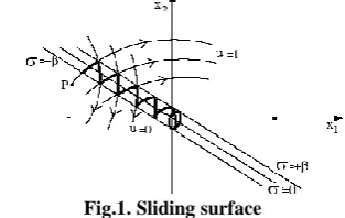
[image:2.595.350.507.280.379.2]

Where β define a suitable hysteresis band. In this way, the phase plane is divided in two regions separated by the sliding line, each associated to one of the two sub topologies defined by switch status u. When the system status is in P, Since we are in the region



 



, the switch is closed and the motion occurs along a phase trajectory corresponding to u=1. When the system status crosses the line



 



, according to (4), u=0 and the system status follows a phase trajectory corresponding to u=1. observing that the phase trajectories, in proximity of the sliding line, are directed toward the line itself, the resulting motion is made by continuous commutations around the sliding line, so that the system status is driven to the final equilibrium point.

Fig.1. Sliding surface

From this example, in the hypothesis of a suitable small value of β, two important conclusions arise

 When the system is in the sliding mode, its evolution is independent of the circuit parameters. It depends only on the sliding line chosen. In the example shown in Fig.3 the dynamic is of the first order with a time constant equal to τ.

 If N is the order of the original system, the dynamic of the controlled system in sliding mode has order N-1, since the state variables are constrained by the equation





0

. Note that the switching frequency is determined by the amplitude of the hysteresis band β. The potentialities of this control technique in the application to switch to switch-mode power supplies are now evident: it exploits the intrinsic non-linear nature of these converters and it is able to provide dynamic behaviors that are different from that of the substructures composing the system, and correspond to that of a reduced system.

2.2. Switching surface design

In the simple case of the second-order systems considered in the previous section, sliding mode control design requires only selection of parameter τ. Selection, must be done in order to ensure the following three constraints The hitting condition, which requires that the system trajectories cross the sliding line irrespective of their starting point in the phase plane; The existence condition, which requires that the system trajectories near the sliding line (in both regions) are directed toward the line itself; The stability condition of the system motion on the sliding line (i.e. the motion must be toward the equilibrium point).

2.3. Existence Condition:

form V x t( , , ) 0.52( )x . To determine the gains necessary to drive the system state to the surface



( )

t



0

, they may be choose so that

2

. _{( )} .

( , , ) 0.5d ( )d x . 0

V x t x

dt dt







 





 

 (5)

Thus sliding mode does exist on a discontinuity surface whenever the distances to this surface and the velocity of its

hange .



are of opposite signs, i.e. when

. 0

lim 0

x





and .

0

lim 0

x

2.4. Stability Condition

Switching surface design is predicted upon knowledge of the system behavior in a sliding mode. This behavior depends on the parameters of the switching surface. In any case, achieving a switching-surface design requires analytically specifying the motion of the state trajectory in a sliding mode. The so called method of equivalent control is essential to this specification. 2.5. Equivalent Control

Equivalent control constitute an equivalent input which, when exciting the system, produces the motion of the system on the sliding surface whenever the initial state is on the surface. Suppose at t1 the plant’s state trajectory intercepts the switching surface, and a sliding mode exists. The existence of

a sliding mode implies that, for all tt₁, ( ( ), ) x t t 0, and hence .( ( ), )x t t 0. Using the chain rule, we define the equivalent control ueq for system of the form eq.3.70 as the

input satisfying

. .

( , ) ( , ) eq 0

x f x t B x t u

t x t x x

    

     

     (6)

Assume that the matrix product _{B x t( , )} x





 is nonsingular

for all t and x, and one can compute ueq as

1

( , ) ( , )

eq

u B x t f x t

t t x

   

  

   

 _{  }  _

  

   

(7)

Therefore, given that



( ( ), )

x t

₁

t

₁



0

, then for all

t



t

₁, the dynamics of the system on the switching surface will satisfy

. 1 1

( ) ( , ) ( , ) ( , ) ( , ) ( , )

x t I B x t B x t f x t B x t B x t

x x x t

     

   

  

   

 _{ }  _{ }

 _{ }  _{ }

   

 

 

(8)

This equation represents the equivalent system dynamics on the sliding surface. The driving term is present when some form of tracking or regulation is required of the controlled system, e.g. when

( , ) . ( ) 0

1 N

x t K x_{i i} r t

    (9)

With r(t) serving as a “reference” signal.

2.6. Physical Meaning of the Equivalent Control

A real control always includes a slow component to which a high rate component maybe added. So decompose the control structure as

( , ) ( , ) ( , )

u x t u_eq x t u_N x t (10) Where ueq is only valid on the sliding surface and uN assures

the existence of a sliding mode. And uN is defined as

( , )

sgn( )

N

u

x t





(11)

Where sgn( ) 





Since a control plant is a dynamic object, its behavior is largely determined by the slow component while its response to the high rate component is negligible. On the other hand, the equivalent control method demands a substitution of the real control in the motion Eq (10) with a continuous function u

eq-(x,t), which does not contain any high rate component. The equivalent control equals the slow component of the real control i.e. average control value and may be measured by a first order linear filter provided its time constant is small enough as compared with the slow component, yet large enough to filter out the high rate component and approximately matched with the boundary layer width.

3.

ADAPTIVE

SLIDING

MODE

CONTROL OF HIGH POWER FACTOR

BOOST RECTIFIER

In this work a new variation of Sliding mode control of High Power Factor Boost rectifier based on Quasi-Steady-State operation of CCM converter is proposed.

3.1 System Model

Taking into account that the cut-off frequency of the filter is much higher the line frequency, the resulting close loop dynamic behavior of the boost Power Factor Correction rectifier can be approximated by the following relations:

sgn(

)

i L in

i



i

V

(12)

.di _{in o}. _eq

L V V u dt 

(13)

. o . o

eq

dV V

C i u dt   R

(14)

Where ueq is the average values of the control variable u (u=0 when switch is on and u=1 when switch is off).

3.2.Controller Design

The input current of a Active Power Factor Correction must fallow the shape the line voltage as a resistor, and simultaneously, the average value of the output voltage

(<V-o>) must be regulated to a reference value (Vo ref). both control

goals be achieved if the input current satisfies the following relation.

in L

eq

V i

R

 (15)

Where iL is the inductor current of the converter and Req is the

emulated resistor the values of which are related to the input power and the output voltage. The value of Req must be

controlled to make the average value <Vo> follow a reference

value Vo ref.

The control scheme consists of both an outer control loop, which regulates the value of the emulated resistor, and an inner control loop, which is used to make the input current

follow a reference value Vin

Req

.

To implement the relation of Eq. (15), avoiding the sensing of the line voltage and the use of an analogue multiplier, the quasi-steady-state approach is considered. According to the approach, the ratio between the line and the output voltage can be approximated by the voltage conversion ratio of a DC/DC boost converter. Therefore, the following relationship can be used in the control design

1

Vo

V_in u

  

(16)

Substituting Eq.(16) for Eq.(15) yields a new expression of the control goal is

.

V_o u

iL Req

 

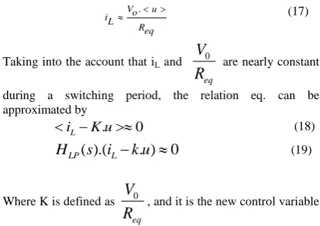
 (17)

Taking into the account that iL and 0

eq

V

R

are nearly constant during a switching period, the relation eq. can be approximated by

.

0

L

i

K u

 



(18)

( ).(

. )

0

LP L

H

s

i



k u



(19)

Where K is defined as 0

eq

V

R

, and it is the new control variable which is used to regulate the output voltage. In order to achieve the unity-power-factor, the expression (18) must be satisfied when the sliding regime is reached. The expression of this required sliding surface can be deduced by identifying the invariance condition





0

with Eq.(18).

( ).(

. )

LP L

H

s

i

k u







(20)

Note that this sliding surface will satisfy the transversal condition if HLP(s) is the first order low pass filter

(HLP(s)=so/s+so), it can be used to calculating the average

value of

i

_L



k u

.

during a switching period. The control law associated with this surface is deduced by using the

reaching condition, .

.

0

 



[7], which yields

1...

0

0...

0

when

u

when









 

_



Moreover, a proportional-integral control of K has been used to make the output voltage be regulated to a reference value Vo ref.

( ) ( )

0 t

K K_p V V_o K_I V V d_o

oref oref 

     (21)

In the design of the SM controller, K is typically set as a constant parameter corresponding to a nominal operating condition, to facilitate practical implementation. This makes the sliding line static irrespective of the operating condition. Strictly speaking, this is an inappropriate approach, which leads to unsatisfactory performance when there is a large deviation in the operating conditions. it is known that K is proportional inversely proportional to load resistance, RL, which may not be constant. Consequently, we can re-express it as:

𝛼 ∝_𝑅1

𝐿 (22)

The reason for introducing an adaptive system into the SM voltage controller is to alleviate the problems associated with the deviation of loading conditions. This is possible by manipulating the relationship of α and RL described in (22), which gives

𝐾 =𝐾(𝑛𝑜𝑚 )𝑅𝐿(𝑛𝑜𝑚 )

𝑅𝐿 (23) where K is the instantaneous sliding line gradient; RL is the instantaneous loading resistance; and RL(nom) and K(nom) are respectively the nominal loading resistance and sliding

line gradient. Since it is not possible to measure resistance directly, the relationship:

𝑅𝐿=

𝑉𝑂

𝑖𝑅

where 𝑖𝑅≠ 0 (24) is exploited to obtain the instantaneous loading resistance. The incorporation of (23) and (24) will result in an adaptive SM controller which will monitor the output voltage and load current, and adjust α accordingly to provide optimal dynamic performances corresponding to any load variation. This can be performed by gain scheduling [8], which effectively generates a value k corresponding to

𝑘 =𝑅𝐿(𝑛𝑜𝑚 )

𝑅𝐿 (25)

The value of k is then used to vary α in the SM voltage controller through a multiplier, i.e.,

[image:4.595.307.541.87.582.2]

K = kK(nom). (26) A block diagram of the proposed adaptive SM voltage controller is illustrated in Fig. 2. It is worth mentioning that this controller can easily be implemented using low cost op- amps and simple analog multiplier/divider ICs.

Fig.2. Block Diagram of proposed controller

4. SIMULATION RESULTS

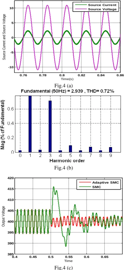
Fig.3. Simulation diagram of proposed controller A Sliding mode controller based on variable structure theory has been simulated. Fig.3 shows the simulation diagram of proposed controller. Simulation is done by using MATLAB/SIMULINK with the help of mathematical model of boost converter. Mathematical model of boost converter is developed by using state space averaging technique. The output voltage of the rectifier is regulated at 400V. The simulation waveforms of the input current (i), input voltage (v

in), at different load conditions are shown in Fig.4.(a) and

[image:4.595.52.282.93.255.2]

output voltage is regulated with low ripple factor under steady-state condition.

Fig.4 (a)

Fig.4 (b)

Fig.4 (c)

Fig.4.Simulation results: (a) are input current and voltage,(b) THD in input current, (c) are output voltage when load is R=250Ω-650Ω at 0.5sec respectively

5. CONCLUSION

The proposed adaptive SM controller alleviates the problem of deteriorated dynamic and steady state performances faced by conventional non-adaptive SM controlled high power factor boost rectifier. This is performed by employing the gain scheduling scheme which monitors the output voltage and load current to vary the sliding line of the system. Simulation results showed that the adaptive SM controlled converter has faster dynamic response when it is operated above the nominal load, and it eliminates overshoots and ringing in the transient response when operated below the nominal load.

6. REFERENCES

[1]. P.Mattavelli, L. Roossetto, G. Spiazzi, “General purpose sliding mode controller for DC-DC converter applications”, PESC’93, pp.609-615.

[2]. P.mattavelli, L. rossetto, L. malesani, “Application of sliding mode control design to Switch-Mode Power Supplies”.

[3]. O. Lopez, L. Garacia de Vicuna and M. Castilla “Sliding Mode Control Design of a Boost High-Power Factor pre-regulator vased on the Quasy-Steady-State Approach”, IEEE Trans. 2001, pp.932-935.

[4]. J.Y.Yung, W. Gao and J.C.Hung, “Variable Structure Control: A Survey”, IEEE Trans. Ind. Electronics, vol 40, pp.2-22.Feb.1993.

[5]. R.A. Decarlo, S.H. Zak, S.V.Drakunov, “Varaible Structure, Sliding Mode Control Design”, Control System Hand Book, pp:941-951.

[6]. K.J. Astrom and B. Wittenmark, Adaptive Control. Reading, Mass.: Addison-Wesley, 2nd ed., 1995.

0.76 0.78 0.8 0.82 0.84 0.86 -10

-5 0 5 10

Time(s)

S

ou

rc

e

C

ur

re

nt

a

nd

S

ou

rc

e

V

ol

ta

ge

Source Current Source Voltage

0.4 0.45 0.5 0.55 0.6 0.65 385

390 395 400 405 410 415 420

Time

O

ut

pu

t

V

ol

ta

ge

[image:5.595.59.271.103.559.2]