Munich Personal RePEc Archive
R-estimation for ARMA models
Allal, Jelloul and Kaaouachi, Abdelali and Paindaveine,
Davy
2001
R-ESTIMATION FOR ARMA MODELS
By J. Allal, A. Kaaouachi and D. Paindaveine
Universit´e Mohamed Ier, Oujda (Morocco)
Universit´e Libre de Bruxelles (Belgium)
ABSTRACT
This paper is devoted to the R-estimation problem for the parameter of a stationary ARMA model. The asymptotic uniform linearity of a suitable vector of rank statistics leads to the asymptotic normality of√
n-consistent R-estimates resulting from the minimization of the
norm of this vector. By using a discretized√
n-consistent preliminary estimate, we construct
a new class of one-step R-estimators. We compute the asymptotic relative efficiency of the proposed estimators with respect to the LS estimator. Efficiency properties are investigated via a Monte-Carlo study in the particular case of an AR(1) model.
KEYWORDS AND PHRASES: R-estimation, ARMA models, local asymp-totic normality, asympasymp-totic linearity.
1
Introduction
R-estimation — estimation methods based on ranks — was initiated by Hodges and Lehmann (1963), who proposed the first R-estimator for location. The theory subsequently has been de-veloped and systematized in the general framework of linear models with independent errors; we refer to the papers by Adichie (1967), Jureˇckov´a (1971), Koul (1971) and Jaeckel (1972), and the monographs by Puri and Sen (1985) and Jureˇckov´a and Sen (1996) for a detailed account and extensive bibliography.
Introducing R-estimation ideas to the context of time series analysis has been much slower. A first successfull attempt has been made by Allal (1991), who proposes a R-estimator for the parameter of a first-order autoregressive (AR(1)) model, based on the serial linear rank statistics introduced by Hallin et al. (1985) and Hallin and Puri (1988). A theory of R-estimation has been developed for higher order AR(p) models by Koul and Saleh (1993); the statistics on which their method relies however are not genuinely rank-based, as they involve both the ranks (of residuals) and the observations themselves.
The purpose of this paper is to investigate the problem of R-estimation in the more general context of ARMA(p, q) models, of the form
where{εt;t∈Z}is white noise with unspecified densityg. Contrary to Koul and Saleh (1993), the
statistics we are using are genuinely rank-based, in the sense that they only depend on the vector of (residual) ranks.
An important tool in our approach is the LAN property of ARMA models for giveng(satisfying mild regularity assumptions). This LAN result was established in Kreiss (1987, a and b). More particularly, we will use a rank-based version of this result, as given in Hallin and Puri (1994).
The paper is organized as follows. Section 2 introduces notation and the main technical as-sumptions. Section 3 presents the asymptotic representation and asymptotic normality results for serial rank statistics to be used in the sequel. Section 4 studies the R-estimation problem in ARMA model. Section 5 gives a method of constructing, with the help of a preliminary √n-consistent estimate of θ0, a class of asymptotic R-estimators. Section 6 provides the asymptotic relative efficiencies of R-estimators with respect to the least-squares estimate. In Section 7, we investigate the finite-sample performance of the proposed estimates via a Monte-Carlo study. The appendix contains details of the proof of Proposition 3.3.
2
Notation and basic assumptions
In this section we introduce a class of serial rank statistics and state the basic assumptions to be made. The ARMA(p, q) model (1) can be written under the form
A(L)Xt=B(L)εt, t∈Z,
where L is the lag operator, A(L) := 1−
p
X
i=1
AiLi and B(L) := 1 + q
X
i=1
BiLi. The parameter θ0 = (A1, ..., Ap, B1, ..., Bq) ∈ Rp+q is chosen in such a way that both the stationarity and the
invertibility conditions are fulfilled.
LetX(n) := (X1(n), . . . , Xn(n)) be an observed series of length n, and denote by Hg(n)(θ0) the
hypothesis under which X(n) is generated by model (1). Denote by R(tn)(θ0) the rank of the
residualZt(n)(θ0) among
n
Z1(n)(θ0), . . . , Z (n)
n (θ0)
o
, where
Zt(n)(θ0) :=
A(L)
B(L)X (n)
t , t= 1, . . . , n.
We suppose that the vector (ε−q+1, . . . , ε0, X−p+1, . . . , X0) is observed, or that Xt(n) = 0,
t ≤ 0. Such assumptions have no influence on asymptotic results. Then, under Hg(n)(θ0),
n
Z1(n)(θ0), . . . , Z (n)
n (θ0)
o
is white noise, with probability density functiong.
Consider the serial rank statistics of orderk(k= 1, . . . , n−1), known as a rank autocorrelation of orderk,
rk(n)(θ0) :=
(
(n−k)−1
n
X
t=k+1
J1
R(tn)(θ0)
n+ 1
!
J2
R(t−kn)(θ0)
n+ 1
!
−m(n)
) ,
σk(n), (2)
where J1 and J2 are score functions, and m(n) and σk(n) are normalizing constants such that (n−k)1/2r(n)
k (θ0) is standardized underH(n)(θ0) (the hypothesis under which the densitygremains
unspecified). See Hallin and Puri (1994), pp. 186-187 for explicit values ofm(n) andσ(n)
Also denote by rk,g(n) the g-rank autocorrelation of order k, i.e., the rank statistic (2) with
J1 :=ϕg◦G−1 and J2:=G−1, whereϕg(.) := −g
′
g (.) andG
−1 denotes the generalized inverse of the cdfGassociated withg.
Throughout the paper we assume that the following assumptions hold for the error density g
and the score functionsJ1 andJ2.
AssumptionsA.1.
(i)
Z
xg(x)dx= 0 and 0< σ2:=
Z
x2g(x)dx <∞.
(ii) g is absolutely continuous, with a.e. derivativeg′, and strongly unimodal.
1. The Fisher informationI(g) :=
Z hg′(x)
g(x)
i2
g(x)dxis finite.
(iii) g(x) > 0 ∀x∈ R and (ε−q+1;. . .;ε0;X−p+1;. . .;X0) possesses a nowhere vanishing joint
densityg0(.,θ) that satisfiesg0(.,θ(n))
−g0(.,θ0) =o
p(1), underHg(n)(θ0), asθ(n)→θ0.
AssumptionsA.2.
(i) J1 and J2 are nondecreasing and square-integrable functions such that 1
Z
0
Ji(u)du = 0,
i= 1,2.
(ii) J1◦GandJ2◦Gare Lipschitz.
Remark 2.1
Assumptions A.1 are used in proving the LAN property. AssumptionA.2(ii) is verified, for example, ifJi= Φ−1(.) andGis normal (Φ(.) stands for the standard normal distribution function),
Ji(u) = 2u−1 andG is normal or logistic orJi(u) = ln(1−uu ) and G is logistic. It easily can be
weakened into a piecewise Lipschitz assumption, which also accomodates such distributions as the double exponential.
3
Asymptotic representation and asymptotic normality
Consider the sequence of local alternatives Hg(n) θ0+n−1/2τ(n), where τ(n) := (γ(n),δ(n)) ∈
Rp+q is such that sup
n
τ(n)′τ(n) < ∞, and denote by nψt(1), . . . , ψ(tp+q);t∈Zo a fundamental system of solutions of the homogeneous equation
A(L)B(L)ψt= 0, t∈Z
Associated with this fundamental system, denote byCψ(θ0) andW2ψ(θ0) the matrices whose
elements areψ(ij) and ∞
X
t=1
ψ(ti)ψ
(j)
t (i, j= 1, . . . , p+q), respectively. Finally, let
M(θ0) :=
1 0 . . . 0 1 0 . . . 0
g1 1 . . . h1 1 . . . ..
. ... ... ...
gp−1 . . . 1 hq−1 . . . 1
gp . . . g1 hq . . . h1 ..
. ... ... ...
gp+q−1 . . . gq hp+q−1 . . . hp
,
wheregiandhiare the Green’s functions associated with the operatorsA(L) andB(L) respectively.
Note that all the above quantities are continuous functions of θ0. In the sequel, the notation
ψ(ti)(θ0),Cψ(θ0),M(θ0) andW2ψ(θ0) will be avoided.
Now define the vector of rank statistics
√
nT(n)(θ0) :=
n−1
X
k=1
(n−k)1/2ψ(1)k (θ0)rk,g(n)(θ0), . . . ,
n−1
X
k=1
(n−k)1/2ψk(p+q)(θ0)rk,g(n)(θ0)
!′
. (3)
Then we can show the following proposition :
Proposition 3.1 (Asymptotic representation) Assume thatA.1 andA.2(i)hold. Then,
(i)n1/2r(n)
k (θ0) =I −1 (J1,J2)n
−1/2
n
X
t=k+1
J1◦G(Zt(n)(θ0))J2◦G(Zt−k(n)(θ0))+op(1), underHg(n)(θ0),
asn→ ∞, whereI2
(J1,J2):=
1
Z
0
[J1(u)]2 du
1
Z
0
[J2(u)]2 du;
(ii) the rank statistics n1/2r(n)
k (θ0)is asymptotically standard normal underH(n)(θ0)
Proof. (i) See Section 4 of Hallin et al. (1985).
(ii) Use (i) and the central limit theorem of k-dependent random variables (See Yoshihara
(1976)). ✷
Proposition 3.2 (Hallin and Puri 1994) Local asymptotic normality.
Assume that A.1 and A.2(i) hold. Let Λ = Λ(θn)
0+n−1/2τ(n)/θ0;g be the log-likelihood ratio for Hg(n)(θ0+n−1/2τ(n))with respect toHg(n)(θ0). Then, underHg(n)(θ0),
Λ =τ(n)′∆(gn)(θ0)−
1 2σ
2I(g)τ(n)′
Γ(θ0)τ(n)+op(1),
asn→ ∞, where
∆(gn)(θ0) :=σ[nI(g)]1/2M′(θ0)C′−ψ1(θ0)T
(n)(
and
Γ(θ0) :=M′(θ0)C′−ψ1(θ0)W2ψ(θ0)C−ψ1(θ0)M(θ0).
Moreover, the limiting distribution of∆(gn)(θ0)under Hg(n)(θ0)isN 0, σ2I(g)Γ(θ0).
Proof. See Proposition 4.1 of Hallin and Puri (1994). ✷
As a consequence we obtain the following corollary.
Corollary 3.1 Assume that A.1 and A.2(i) hold. Then, the following properties hold : (i) The limiting distribution of ∆(gn)(θ0) − σ2I(g)Γ(θ0)τ(n) under H
(n)
g (θ0 + n−1/2τ(n)) is
N 0, σ2I(g)Γ(θ0)
.
(ii) The limiting distribution of n1/2r(n)
k (θ0) under H
(n)
g (θ0 + n−1/2τ(n)) is
Nc(J1, J2, g)(ak(n)+b(kn)),1
, where
c(J1, J2, g) :=I(−J11,J2) 1
Z
0
J1(u)ϕg◦G−1(u)du
1
Z
0
J2(u)G−1(u)du.
and
a(kn):=
p
X
j=1
γj(n)gk−j and b(kn):= q
X
j=1
δ(jn)hk−j.
Proof. (i) This follows by applying Le Cam’s third lemma (see H´ajek and ˇSid´ak (1967)) in Proposition 3.2.
(ii) The asymptotic normality under Hg(n)(θ0+n−1/2τ(n)) follows by piecing together Proposi-tion 3.1, the asymptotic joint normality of n1/2r(n)
k (θ0),Λ
(n)
θ0+n−1/2τ(n)/θ0;g
under Hg(n)(θ0),
and Le Cam’s third lemma. ✷
Let us now turn to asymptotic uniform linearity of the rank autocorrelation coefficients :
Proposition 3.3 Assume that A.1 andA.2 hold. Then, for all kand all c >0, underHg(n)(θ0),
asn→ ∞,
sup
kτ(n)k≤c
n
1/2hr(n)
k (θ0+n
−1/2τ(n))
−r(kn)(θ0)i+c(J1, J2, g)(a(kn)+b(kn))
=op(1). (4)
The proof is rather technical and we defer it to the Appendix.
4
Estimators based on ranks
4.1
Definition of the R-estimators
Define the vector of rank statistics
√
nT(Jn1),J2(θ0) :=
n−1
X
k=1
(n−k)1/2ψ(1)k (θ0)rk(n)(θ0), . . . ,
n−1
X
k=1
(n−k)1/2ψk(p+q)(θ0)r(kn)(θ0)
!′
and put
∆(Jn1),J2(θ0) :=n
1/2M′
(θ0)C′−ψ1(θ0)TJ(n1),J2(θ0).
Obviously, when the scoresJ1(.) andJ2(.) areϕg◦G−1(.) andG−1(.) respectively, we obtain the
central sequence up to a positive factor. More precisely,
∆(gn)(θ0) =σI1/2(g)∆
(n)
ϕg◦G−1,G−1(θ0).
It easily follows from Proposition 3.1 that the vector∆(Jn1),J2(θ0) is asymptotically normal, under
Hg(n)(θ0), with mean zero and covariance matrix Γ(θ0). This suggests estimating the unknown
parameterθ0 by the value ofθfor which ∆J(n1),J2(θ) is as near to zero as possible, i.e., to estimate
θ0 by
¯
θ(n):= arg min
θ k∆
(n)
J1,J2(θ)k, (5)
wherek.kis any standard norm inRp+q.
4.2
Asymptotic uniform linearity
In this subsection we give the asymptotic uniform linearity of∆(Jn1),J2(θ0+n−1/2τ(n)) inkτ(n)k ≤ c.
Proposition 4.1 Assume that A.1 andA.2hold. Then for allc >0, underHg(n)(θ0), asn→ ∞,
sup
kτ(n)k≤c
∆
(n)
J1,J2(θ0+n
−1/2τ(n))−∆(n)
J1,J2(θ0) +c(J1, J2, g)Γ(θ0)τ
(n)
=op(1). (6)
Proof. Fors= 1, . . . , p+q, denote byTJ(1n,J)s2(.) thesth component of √
nT(Jn1),J2(.). We proceed by proving that
sup
kτ(n)k≤c
T
(n)s
J1,J2(θ0+n
−1/2τ(n))
−TJ(1n,J)s2(θ0) +c(J1, J2, g)
∞
X
k=1
ψk(s)(θ0)(ak(n)+b(kn))
=op(1),
underHg(n)(θ0), asn→ ∞. We have
TJ(n1,J)s2(θ0+n−1/2τ(n))−TJ(n1,J)s2(θ0) +c(J1, J2, g)
∞
X
k=1
ψk(s)(θ0)(ak(n)+b(kn)) = (7)
n−1
X
k=1
ψk(s)(θ0)
n
(n−k)1/2hrk(n)(θ0+n−1/2τ(n))−r(kn)(θ0)
i
+c(J1, J2, g)(a(kn)+b
(n)
k )
o
+c(J1, J2, g)
∞
X
k=n
ψk(s)(θ0)(ak(n)+b(kn))
+
n−1
X
k=1
(n−k)1/2hψ(ks)(θ0+n−1/2τ(n))−ψ(ks)(θ0)
i
Since the AUL result of Proposition 3.3 holds uniformly over the set{k= 1, . . . , n−1}, the first term of the right side of (7) is ¯op(1), asn→ ∞, where ¯op(1) stands for some sequence converging to
zero uniformly over the set
kτ(n)k ≤c . The particular form ofak(n)andb(kn), and the exponential decrease inkofψk(s)(.) imply that the second term of the right side of (7) converges to 0, uniformly in kτ(n)k ≤c as n → ∞. The exact variance of the third term, under Hg(n)(θ0+n−1/2τ(n)), is bounded by
∞
X
k=1
h
ψk(s)(θ0+n−1/2τ(n))−ψk(s)(θ0)
i2
+
∞
X
k=1
ψ
(s)
k (θ0+n−1/2τ(n))−ψ(ks)(θ0)
!2
.
This latter quantity is o(1) as n → ∞; indeed, supn ψ
(s)
k (θ)
:s= 1, . . . , p+q;θ∈K o
≤ A bi,
where A > 0, 0 < b < 1 and K is a compact set in Rp+q, and θ 7→ ψ(ks)(θ) is continuous. Consequently, under Hg(n)(θ0), hence also, due to contiguity, under Hg(n)(θ0+n−1/2τ(n)), the third term on the right side of (7) is ¯op(1), asn→ ∞. This completes the proof of (6).
The end of the proof is obvious, becauseM(θ0+n−1/2τ(n)) andCψ(θ0+n−1/2τ(n)) converge respectively toM(θ0) andCψ(θ0), uniformly inkτ(n)k ≤c.
✷
4.3
Asymptotic normality of R-estimates
This subsection gives the limit law of R-estimates.
Proposition 4.2 Assume that A.1 andA.2 hold. Let (¯θ(n)) be a √n-consistent solution of (5), then the asymptotic distribution of√n¯θ(n)−θ0
underHg(n)(θ0)isN 0, c−2(J1, J2, g)Γ−1(θ0).
Proof. From Proposition 3.1, the vector ∆(Jn1),J2(θ0) is asymptotically normal with mean 0 and covariance matrix Γ(θ0), under H(n)(θ0). The result follows from the Cram´er-Wald device and Proposition 4.1. ✷
Proposition 4.3 Assume that A.1 and A.2 hold, and suppose that λ′∆J(n1),J2(θ0+b n
−1/2λ) is monotone in bfor everykλk= 1. Then, for any solution(¯θ(n))of (5), the asymptotic distribution of √nθ¯(n)−θ0
underHg(n)(θ0)isN 0, c−2(J1, J2, g)Γ−1(θ0).
Proof. The proof proceeds along the same lines as in Jureˇckov´a (1971). ✷
However, it is not easy to prove the√n-consistency of any solution of (5), or to find reasonable assumptions ensuring the monotonicity inbofλ′∆(Jn1),J2(θ0+b n−1/2λ). That is why we propose the following construction of R-estimators, that allows for trivial asymptotic properties and achievable local and asymptotic optimality.
5
Construction of asymptotic R-estimates
In this section we adopt the Le Cam-H´ajek approach to construct a class of asymptotic R-estimators ˆ
θ(n)satisfying
∆(Jn1),J2(ˆθ(n)) =op θ0
For this purpose, let (˜θ(n)) denote a discretized√n-consistent preliminary estimate of θ0, i.e., a sequence of estimates such that
(i)√n˜θ(n)−θ0
=Op θ0
(1), as n→ ∞,
(ii) the number of possible values of ˜θ(n)in balls of the form
θ∈Rp+q :√nkθ−θ0k ≤c , c >0 fixed remains bounded, asn→ ∞.
The √n-consistent condition is satisfied by all estimates that are usually considered in the context of ARMA models (see for example Fuller (1976)), and the discreteness condition goes back to Le Cam and has been useful in a variety of problems connected with the analysis of time series data.
Proposition 5.1 Assume thatA.1 andA.2 hold. Define
ˆ
θ(n)= ˜θ(n)+√1 nc
−1(J
1, J2, g)Γ−1(˜θ (n)
)∆(Jn1),J2(˜θ(n)). (8) Then,
√
n(ˆθ(n)−θ0) =c−1(J1, J2, g)Γ−1(θ0)∆J(n1),J2(θ0) +opθ 0
(1), (9)
and the asymptotic distribution of√nˆθ(n)−θ0
underHg(n)(θ0)isN 0, c−2(J1, J2, g)Γ−1(θ0)
. In addition
∆(Jn1),J2(ˆθ
(n) ) =op
θ0
(1).
Finally, the sequence of estimators(ˆθ(n))associated with the scoresJ1:=ϕg◦G−1andJ2:=G−1 is locally and asymptotically minimax under the innovation density g.
Proof. SinceΓ(˜θ(n)) is consistent forΓ(θ0), we have
√
nˆθ(n)−θ0
−c−1(J1, J2, g)Γ−1(θ0)∆(Jn1),J2(θ0)
=√nθ˜(n)−θ0
+c−1(J1, J2, g)Γ−1(θ0)
∆(Jn1),J2(˜θ
(n)
)−∆(Jn1),J2(θ0)
+op θ0
(1),
which, in view of Proposition 4.1, is aop θ0
(1). The end of the proof is straightforward. ✷
The following corollary shows that ˆθ(n) and ¯θ(n)are asymptotically equivalent.
Proposition 5.2 Assume that A.1 andA.2 hold. Let (¯θ(n)) be a √n-consistent solution of (5). Then
√
nˆθ(n)−θ¯(n)=op(1),
under Hg(n)(θ0).
Proof. The desired result readily follows from the fact that both ˆθ(n)and ¯θ(n) satisfy (9). ✷
Score functions Density types
J1(u)J2(v) Normal Logistic Double-exp.
van der Waerden 1.000 1.048 1.226
Φ−1(u)Φ−1(v)
Wilcoxon 0.948 1.098 1.482
(2u−1) ln( v
1−v)
Laplace 0.612 0.812 2.000
sign(2u−1)F−1
e (v)
Figure 1: Asymptotic relative efficiencies of the proposed R-estimator (for van der Waer-den, Wilcoxon and Laplace scores) w.r.t. the LS-estimator under normal, logistic and double-exponential innovation densities.
6
Asymptotic relative efficiencies
We now compute theAREof the proposed estimators with respect to the usual Gaussian estimator, namely the LS estimator. TheseAREsare obtained as the ratios of the asymptotic variances of the considered estimators. The asymptotic variance-covariance matrix of the proposedR-estimate ˆθ(n)
is given in Proposition 5.1, and it is well-known that the asymptotic variance-covariance matrix of the LS estimate ˆθ(LSn)is Γ−1(θ0). Therefore, the AREof ˆθ(n)w.r.t. ˆθ(LSn)is given by
AREg(ˆθ
(n)
/θˆ(LSn)) =c2(J1, J2, g).
Figure 1 summarizes the numerical values of the AREs of the proposed R-estimator w.r.t. the least-squares estimator for various score functions and density types.
Figure 1 illustrates the gains of efficiency achievable by using R-estimator. Note that, when using van der Waerden scores, theAREs are uniformly larger than or equal to one. This result was established by Chernoff and Savage (1958) for linear models with independent errors and extended to the ARMA case by Hallin (1994).
Proceeding as above, we can check that theARE of the proposed R-estimator w.r.t. the LAM (locally and asymptotically minimax) estimator (i.e., the one based on the scoresJ1:=ϕg◦G−1
andJ2:=G−1 underHg(n)(θ0)) is given by
AREg(ˆθ
(n)
/ˆθ(LAM,gn) ) =c2(J1, J2, g)σ−2I−1(g).
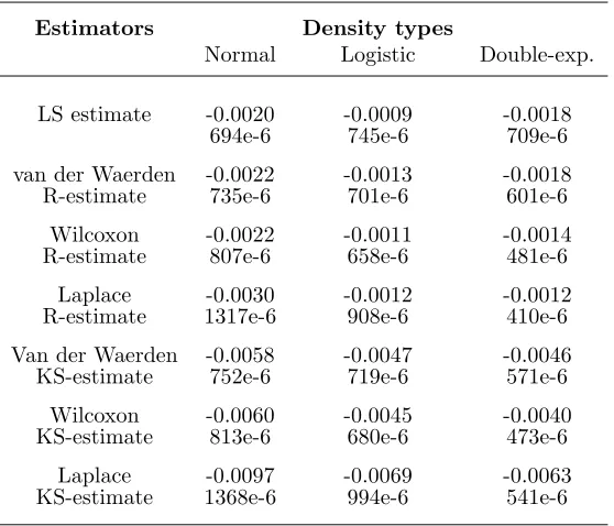
7
Simulation results
[image:10.595.139.431.125.276.2]Estimators Density types
Normal Logistic Double-exp.
LS estimate -0.0020 -0.0009 -0.0018
694e-6 745e-6 709e-6
van der Waerden -0.0022 -0.0013 -0.0018
R-estimate 735e-6 701e-6 601e-6
Wilcoxon -0.0022 -0.0011 -0.0014
R-estimate 807e-6 658e-6 481e-6
Laplace -0.0030 -0.0012 -0.0012
R-estimate 1317e-6 908e-6 410e-6
Van der Waerden -0.0058 -0.0047 -0.0046
KS-estimate 752e-6 719e-6 571e-6
Wilcoxon -0.0060 -0.0045 -0.0040
KS-estimate 813e-6 680e-6 473e-6
Laplace -0.0097 -0.0069 -0.0063
[image:11.595.147.426.124.363.2]KS-estimate 1368e-6 994e-6 541e-6
Figure 2: Simulation results.
independentlyM = 300 series ofn= 500 observations from an AR(1) model with parameterθ0=
ρ0= 0.8 and standard normal, logistic and double-exponential innovation densities, respectively. For each series, we computed the following seven estimators ofρ0: Koul and Saleh’s estimator (for van der Waerden, Wilcoxon and Laplace scores), our one-step estimator (for van der Waerden, Wilcoxon and Laplace scores), and the LS estimator. For each estimate, we report the mean deviation 1
M
PM
m=1ρˆ (n)
m −ρ0and the mean square errorM1 PMm=1(ˆρ (n)
m −ρ0)2. Results are presented
in Figure 2.
Figure 2 confirms the hierarchy of theAREs in Figure 1. Note, in particular, that correctly specified scores lead to the most efficient estimators. The proposed estimators compete very well w.r.t. Koul and Saleh’s estimators (see Koul and Saleh (1993)).
8
Appendix
We now prove Proposition 3.3. Along the same lines as in the proof of Proposition 5.1 of Hallin and Puri (1994), we show that underHg(n)(θ0),
n1/2hr(kn)(θ0+n−1/2τ(n))−rk(n)(θ0)
i
+c(J1, J2, g)(a(kn)+b
(n)
k ) =op(1), (10)
asn→ ∞.
Using the asymptotic representation in Proposition 3.1, one could obtain
˜
rk(n)(θ0+n−1/2τ(n))−r˜k(n)(θ0) +Ic(J1, J2, g)(a(kn)+b
(n)
k ) =opθ
0
(1), as n→ ∞, (11)
where
˜
rk(n)(.) =n−1/2
n
X
t=k+1
J1◦G(Zt(n)(.))J2◦G(Zt−k(n)(.)).
Letε >0. As in Kreiss (1987,b), we decompose the set B ={τ ∈Rp+q :kτk ≤c} into the hypercubes whose vertices are at the points ε(j1, ..., jp+q), ji = 0,±1, ...,±N(ε), i= 1, ..., p+q.
For each τ ∈ B, let τ∗ denote the vertex nearest to zero of the sub-cube containing τ and we adopt the notationsθ=θ0+n−1/2τ andθ∗=θ0+n−1/2τ∗.
From (11) we have
sup
kτk≤c
r˜
(n)
k (θ ∗
)−˜rk(n)(θ0) +Ic(J1, J2, g)(a(kn)∗+b
(n)∗ k )
=opθ
0
(1), as n→ ∞, (12)
where a(kn)∗ and bk(n)∗ are associated with τ∗. Considering an arbitrary hypercube B∗ in the
decomposition, we have
sup
τ∈B∗ r˜
(n)
k (θ ∗)
−˜rk(n)(θ) +Ic(J1, J2, g)(a(kn)∗+b
(n)∗ k −a
(n)
k −b
(n)
k )
≤U
(n)+V(n), (13)
where
V(n)= sup
τ∈B∗
Ic(J1, J2, g)(a
(n)∗ k +b
(n)∗ k −a
(n)
k −b
(n)
k )
≤I|c(J1, J2, g)|(p+q)ε, (14)
U(n) = sup
τ∈B∗ ˜r
(n)
k (θ ∗)
−r˜(kn)(θ) = sup τ∈B∗ n
−1/2
n
X
t=k+1
J1◦G(Zt(θ∗))J2◦G(Zt−k(θ∗))−J1◦G(Zt(θ))J2◦G(Zt−k(θ))
≤ Uk,(n1)+Uk,(n2),
where
Uk,(n1)= sup
τ∈B∗ n
−1/2
n
X
t=k+1
[J1◦G(Zt(θ∗))−J1◦G(Zt(θ))]J2◦G(Zt−k(θ∗))
,
and
Uk,(n2)= sup
τ∈B∗ n
−1/2
n
X
t=k+1
[J2◦G(Zt−k(θ∗))−J2◦G(Zt−k(θ))]J1◦G(Zt(θ))
.
Kreiss (1987b, equation (2.3)) shows that
where z(θ)(t−1,θ∗
) :=
t
X
s=1
h∗s−1(Xt−s, ..., , Xt−s+1−p, Zt−s(θ), ..., Zt−s+1−q(θ))′ (here the (h∗i)’s
denote the Green’s functions associated with the operator B∗[L] := 1 +
q
X
i=1
Bi∗Li). From this
identity and assumption A.2(ii),Uk,(n1)is bounded by
n−1H1(p+q)ε sup
τ∈B∗
n
X
t=k+1
kz(θ)(t−1,θ∗)k
J2◦G(Zt−k(θ
∗))
, (15)
whereH1is the Lipshitz constant forJ1◦G. Now consider the maximum over all hypercubes ofB. We have
Eθ0maxB∗ sup
τ∈B∗ z
(θ)(t
−1,θ∗) 2 ≤ p−1 X i=0
Eθ0max
B∗ τsup∈B∗ " t
X
s=1
h∗s−1Xt−s−i
#2
+
q−1
X
i=0
Eθ0max
B∗ τ∈Bsup∗ " t
X
s=1
h∗s−1Zt−s−i(θ)
#2
.
The first term can be bounded by
t
X
s=1
[max suph∗s−21]Eθ0[X1]
2, which isO(1) uniformly int, because
of Lemma 5.1 of Kreiss (1987,b). The second term can be bounded by
O(1) +Eθ0max sup[
t
X
s=1
h∗s−1(θ0−θ)z(θ0)(t−s−k−1,θ)]2, which is O(1) +O(
ε2
n).
It follows that Eθ0maxB∗ sup
τ∈B∗k
z(θ)(t−1,θ∗)k2 = O(1) uniformly in t. Similarly, using the inequality [J2◦G(Zt−k(θ∗))]2 ≤2[J2◦G(Zt−k(θ∗))−J2◦G(Zt−k(θ0))]2+ 2[J2◦G(Zt−k(θ0))]2,
we obtain thatEθ
0maxB∗τ∈Bsup∗[J2◦G(Zt−k(θ
∗))]2=O(1), uniformly int.
The Cauchy-Schwarz inequality applied to (15) then yields
Eθ
0maxB∗ U
(n)
k,1 =ε O(1). (16) Analogous to (16), one obtains
Eθ
0maxB∗ U
(n)
k,2 =ε O(1). (17) Piecing together (13), (14), (16), and (17) we thus have, asn→ ∞,
max
B∗ τsup
∈B∗ r˜
(n)
k (θ ∗
)−r˜(kn)(θ) +Ic(J1, J2, g)(ak(n)∗+b(kn)∗−ak(n)−b(kn))
=opθ
0
(1). (18)
References
Adichie, J.N. (1967). Estimation of regression parameters based on rank tests,Ann. Math. Statist.
38, 894-904.
Allal, J., (1991). R-estimation dans le mod`ele autor´egressif d’ordre un, Th`ese de Doctorat. Uni-versit´e libre de Bruxelles.
Chernoff, H. and Savage, I.R., (1958). Asymptotic normality and efficiency of certain nonparamet-ric tests. Ann. Math. Statist. 29, 972-994.
Fuller, W.A., (1976). Introduction to statistical time series,J. Wiley, New York.
H´ajek, J. and ˇSid´ak, Z., (1967). Theory of rank tests,Academic press, New York.
Hallin, M., (1994). On the Pitman-nonadmissibility of correlogram-based methods. Journal of Time Series Analysis15, 607-612.
Hallin M., Ingenbleek, J.F. and Puri M.L., (1985). Linear serial rank tests for randomness against ARMA alternatives,Ann. Statist. 13, 1156-1181.
Hallin, M. and Puri, M.L., (1994). Aligned rank tests for linear models with autocorrelated error terms,J. Multivariate Anal. 50, 175-237.
Hodges, J.L. and Lehmann, E.L., (1963). Estimates of location based on rank tests,Ann. Math. Statist. 34, 589-611.
Jaeckel, L.A., (1972). Estimating regression cœfficients by minimizing the dispersion of the resid-uals,Ann. Math. Statist. 43, 1449-1458.
Jureˇckov´a, J. (1971). Nonparametric estimate of regression cœfficients,Ann. Math. Statist. 42, 1328-1338.
Jureˇckov´a, J. and Sen, P.K. (1996), Robust statistical procedures : asymptotics and interrelations.
Koul, H.L., (1971). Asymptotic behavior of a class of confidence regions based on ranks in regres-sion,Ann. Math. Statist. 42, 466-476.
Koul, H.L. and Saleh, A.K.Md.E., (1993). R-estimation of the parameters of autoregressive AR(p) models, Ann. Statist. 21, 534-551.
Kreiss, J.P., (1987-a). On adaptive estimation in stationary ARMA processes, Ann. Statist. 15, 112-133.
Kreiss, J.P., (1987-b). A note on M-estimation in stationary ARMA processes,Statistics and De-cisions3, 317-336.
Le Cam, L., (1960). Locally asymptotically normal families of distributions. University of Cali-fornia. Publications in Statistics,3, 37-98.
Puri, M.L. and Sen, P.R. (1985), Nonparametric methods in general linear models.
J. Allal and A. Kaaouachi, D. Paindaveine,
D´epartement de Math´ematiques, Universit´e Libre de Bruxelles,
Universit´e Mohamed Premier, D´epartement de Math´ematique et ISRO
Oujda 60000. Maroc Campus de la Plaine, CP 210,
Fax: 212 6 50 06 03 1050 Bruxelles, Belgium