The Exact Formulation of the Inverse of the Tridiagonal Matrix for Solving the 1D Poisson Equation with the Finite Difference Method

(1)

http://dx.doi.org/10.4236/jemaa.2014.610030

The Exact Formulation of the Inverse of

the Tridiagonal Matrix for Solving the

1D Poisson Equation with the Finite

Difference Method

Serigne Bira Gueye

Département de Physique, Faculté des Sciences et Techniques, Université Cheikh Anta Diop, Dakar-Fann, Sénégal

Email: [email protected]

Received 21 June 2014; revised 15 July 2014; accepted 8 August 2014

This work is licensed under the Creative Commons Attribution International License (CC BY). http://creativecommons.org/licenses/by/4.0/

Abstract

A new method for solving the 1D Poisson equation is presented using the finite difference method. This method is based on the exact formulation of the inverse of the tridiagonal matrix associated with the Laplacian. This is the first time that the inverse of this remarkable matrix is determined directly and exactly. Thus, solving 1D Poisson equation becomes very accurate and extremely fast. This method is a very important tool for physics and engineering where the Poisson equation ap-pears very often in the description of certain phenomena.

Keywords

1D Poisson Equation, Finite Difference Method, Tridiagonal Matrix Inversion, Thomas Algorithm, Gaussian Elimination, Potential Problem

1. Introduction

The finite difference method is a very useful tool for discretizing and solving numerically a differential equation. It is effectively a classical method of approximation based on Taylor series expansions that has help during the last years theoretical results to gain in accuracy, stability and convergence.

(2)

domi-nant, can be inverted with methods such as Gauss elimination, Thomas Algorithm Method [1]. These technics are powerful and very efficient.

We proposed here, a new and direct method of inversion of this tridiagonal matrix independently of the right- hand side. For Dirichlet-Dirichlet boundary problems, this innovative method is faster than the Thomas Algo-rithm. It gives better accuracy and is far more economical in terms of memory occupation.

First, the finite difference method is presented for the 1D Poisson equation. Secondly, the properties of the matrix associated with the Laplacian and its inverse are discussed. Then, the inverse matrix is determined and its properties are analyzed. Thus, verification is done considering an interesting potential problem, and the sensibil-ity of the method is quantified.

2. Finite Difference Method and 1D Poisson Equation

We consider a function Φ

( )

x which satisfies the Poisson equation ∆Φ

( )

x = f x

( )

, in the interval ] , [a b , where f is a specified function. Φ

( )

x fulfills the Dirichlet-Dirichlet boundary conditions Φ

( )

a = Φa and

( )

b b

Φ = Φ . We consider an one-dimensional mesh with N+2 discrete points

( )

xi . Each point

( )

xi is de-

fined by x_i = + ⋅ ∆a i x, where

(

)

1

b a

x h

N

−

∆ = =

+ being the step size. We define Φ ≈ Φi

( )

xi , fi = f x

( )

i , 0,1, , 1

i=  N+ .

We have chosen the centered difference approximation

(

_O

( )

_∆_x2

)

_{, in this work, for the fact that it gives a}

tri-diagonal, diagonally dominant, and symmetric matrix. Considering all the above mentioned criteria, one can re-write the 1D Poisson equation in a set of algebraic equations:

2

1 2 1 , 1, 2, , . i− i i+ h fi i N

Φ − Φ + Φ = = _ (1)

One gets a linear system of N equations, which can be written in a matrix form [2]

2

1 1

2

2 2

2

3 3

2 4

5

1

: :

2 1 0 0 0 0 1 2 1 0 0 0 0 1 2 1 0 0 0 0 1 2 1 0 0 0 0 1 2

0

0 0 0 0 1

0 0 0 0 0 0 1 2

a

N N

h f h f h f h

−

= =

Φ

−   − Φ

 

 

 ₋  _Φ

 

 −  Φ

 

Φ

− _ _

 _× ₌

 

 ₋  _Φ

 

  _Φ

 

 ₋   _Φ 

   

Φ  

          



      

  

A

4 2

5

2 1 2

: N N b

f h f

h f h f

−

=

 

 

 _{− Φ} 

 





F

(2)

Thus, solving the 1D Poisson equation means to invert the negative definite, and regular N×N-matrix

( )

aij

=

A . Its inverse, that we noted B=

( )

b_ij , is also symmetric. Both matrices have the following properties:

2,

1, 1 0, 1

ij

i j

a i j

i j

− =



=_ − =

 _{− >}



(3)

and

1

1 2

1 1

1

2

2 , 1 , 2

i i i j ij ij ij i

N iN iN i

b b

b b b j N

b b

δ δ δ

− +

−

− + =

 ₋ ₊ ₌ _{< <}



 ₋ ₌



(4)

where

δ

ij is the Kronecker’s delta.

3. The Inverse of Matrix

A

(3)

(

)

1 1 and 1 1 ij ij i ij i

b+ =b +b b = jb + −j (5)

with (5), one sees that the matrix B is entirely determined if the term b₁₁ is known. This term can be deter-mined by observing the behavior of B for different N values: It holds

11=

1 N b

N −

+ (6) From (5) and (6), we get

(

)

(

)

1

1 1

j

i

N j

b

N

N i

b

N

− −

 = −

 +



− −

 _{= −}

 ₊



(7)

Now, the matrix B is completely and exactly determined. B=

( )

bij ; ,i j=1, 2,,N with

(

)

(

)

1 ,

1 _;

1 , 1

ij

N i

j i j

N b

N j

i i j

N  _ − − _

− ≥



 +

= 

− −

 

 ₋  _<

 ₊



(8)

(

)

(

)

(

)

(

)

(

)

(

)

(

)

(

)

(

)

(

)

(

)

(

)

(

)

(

)

(

)

(

) (

)

(

)

(

) (

)

(

)

(

)

1 2 1 3 2 1

1 2 1 2 2 2 1 6 4 2

2 2 2 3 2 3 1 9 6 3

1

1 2 1 3 1 1 3 2

1

3 6 9 3 3 2 2 2 2

2 4 6 2 2 2 2 1 1

1 2 3 2 1

N N N N j

N i N i N i i N i i i i

N

j N N N

=

− − − −



 ₋ ₋ ₋ _ ₋ ₋ _

 



 ₋ ₋ ₋ _ ₋ ₋ _

 

  − 

− − − − − − − −

       

        

+  

− − −

− −



 

        

 

        

 

B

,          

 

 _

The solution of the 1D Poisson equation is obtained with a simple, extremely fast matrix multiplication:

=

Φ BF. Thus, the numerical resolution of the 1D Poisson equation which is an interesting topic in physics and engineering is made easy and very accurate.

Analysis

A first analysis of the matrix

( )

B let us believe that, this new method possesses an algorithm complexity of

( )

(

2

)

O N , which is situated between the Gauss eliminations

(

( )

3

)

O N and the one of Thomas’s

(

O N

( )

)

[1]. A deeper analysis of the matrix

( )

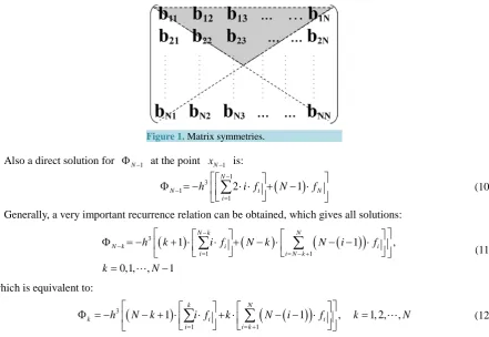
B shows that the complexity brought by the Thomas method is largely improved in this study. In addition, one can see a close link between its row vectors and column vectors.

The matrix

( )

B is also persymmetric:

1, 1 ij N j N i b =b _{− +} _{− +}

All the information about it, can be found in the upper triangle (in gray color, see Figure 1).

Further, we can even find very interesting relations in this matrix which can help refining the final solution. That is what we effectively did, and one can see a direct solution for Φ_N at the point x_N, which can be ex-pressed by

3

1 N

N i

i h i f

=

(4)

[image:4.595.93.535.84.388.2]

Figure 1. Matrix symmetries.

Also a direct solution for Φ_N₋₁ at the point x_N−₁ is:

(

)

1 3 1

1

2 1

N

N i N

i

h i f N f

−

=

  

Φ = − __ ⋅ ⋅ _+ − ⋅ _

 



∑

 (10)

Generally, a very important recurrence relation can be obtained, which gives all solutions:

(

)

(

)

(

)

3

1 1

1 1 ,

0,1, , 1

N k N

N k i i

i i N k

h k i f N k N i f

k N

− −

= = − +

    

Φ = − _ + ⋅_ ⋅ _+ − ⋅_ − − ⋅ __

   

 

= −

∑



(11)

which is equivalent to:

(

)

(

( )

)

3

1 1

1 1 , 1, 2, ,

k N

k i i

i i k

h N k i f k N i f k N

= = +

    

Φ = − _ − + ⋅_ ⋅ _+ ⋅_ − − ⋅ __ =

   



∑

  (12)

This very innovative Equation (12) gives directly and accurately all the solution that we are looking for. It proves that our method is direct, faster than the one of Thomas’s in this context and gives as well better accuracy. Furthermore, it is far more economical in terms of memory occupation. This is due to the fact that the matrix

( )

B does not necessitate to be generated. A programmer does not need to declare nor to define the matrix

( )

B

in his code.

In conclusion to this, we can say that the matrix

( )

B is the key of this efficient new method. This matrix

( )

B , which is the inverse of matrix

( )

A , is determined explicitly, directly, and independently of the right-hand side of the Poisson equation.

N.B.: One can prove using mathematical induction that det

( ) ( ) (

A = −1N N+1

)

. It holds for the

( )

i j,

co-factor of A: 1

(

)

( 1)N 1 ,

ij

CofA = − + j⋅_N− −i _ i≥ j. We call the matrix B Bira’s Matrix.

4. Verification with a Potential Problem

We consider a scalar potential Φ

( )

x , defined in [0, 1], which satisfies

( )

2

( )

2

(

)

2 cos π 1 2

x

x f x x

x ∂ Φ

∆Φ = = = − −

∂ . Φ

( )

x fulfills the following boundary conditions: Φ

( )

0

( )

1 0

= Φ = . The exact solution is

( )

2

2 exact

1 cos π

2

4 2π 4

x

x x

x

   ₋    _ _

 

 

Φ = − + +

 

 

(13)

With the finite difference method, we take N=100, 1 1 x h

N ∆ = =

+ , xi= ⋅ ∆i x , Φ ≈ Φi

( )

xi , and

2 1

( ) cos π 2

i i i

f = f x = − _ _x − __

 

(5)

2 1 1 2 2 2 2 3 3 2 4 4 2 5 5 2 99 99 2 100 100

100 99 98 3 2 1

99 198 196 6 4 2

1

101

3 6 9 294 196 98

2 4 6 196 198 99

1 2 3 98 99 100

h f h f h f h f h f h f h f

Φ  

 

   

 _Φ 

  

 

  

 Φ 

  

 

Φ −   

 _{ =} _×

  

 _Φ 

  

 

  

 

  

_Φ 

  

  _ _

_Φ  

                                ,           (14)

Discussions

We define the variable

ε

i

( )

100 , which is the relative error at point xi for

(

N=100

)

. ΦiFDM represents i

Φ .

Generally, we have

( )

FDM exact

exact

i i

i

N

ε = Φ − Φ

Φ (15)

We can also define the average value of the relative error for a given N:

ε

( )

N . For N =100, it is:

( )

5

100 6.160 10

ε

_≈ _× −

.

We obtain the following results, presented in Table 1.

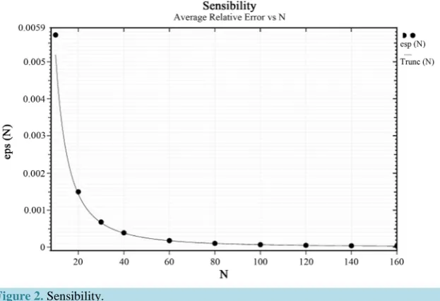
The table shows that the solution is very accurate. Notwithstanding that we have been interested in determin-ing the sensibility of the proposed method. Effectively, we have plotted

ε

( )

N for different N values.

We obtain a hyperbola, which can be predicted as proportional to h2=1

(

N+1

)

2 = ∆x2.

This curve is fitted with a function which can be defined as

( )

(

)

2 2 Trunc , 1 N h N α α = ⋅ =

+ (16)

where

α

≈0.62598. We obtain two curves represented in Figure 2.

Table 1. Results and relative error.

FDM exact (100)

1 9.90099009900990 003 2.47532050462650 003 2.47531263320003 003 3.1799726459536950 0006 2 1.98019801980198 002 4.95054591793065 003 4.95051434685110 003 6.3773332093484231 0006 3 2

i i i i

i x

E E E E

ε

Φ Φ

− − − −

.97029702970297 002 7.42539189910138 003 7.42532094619246 003 9.5555342911444034 0006 4 3.96039603960396 002 9.89938595762298 003 9.89926009306004 003 1.2714542476634171 0005 5 4.95049504950495 002 1.23

E E E E

E

− − − −

− 718692811413 002 1.23716731875297 002 1.5850209475913139 0005 6 5.94059405940594 002 1.48419992841306 002 1.48417179157622 002 1.8957938019221409 0005

7 6.93069306930693 002 1.73087528675008 002 1.73083

E E E

E E E E

E E

− − −

− − − −

− − 715085596 002 2.2033207515521614 0005 8 7.92079207920792 002 1.97709303765360 002 1.97704346980271 002 2.5071705121898528 0005 9 8.91089108910891 002 2.22271602418517 002 2.22265363570344 002 2.80693674

E E

E E E E

E E E

− −

− − − −

− − − 98980424 0005

10 9.90099009900990 002 2.46759042854172 002 2.46751388035270 002 3.1022394496623757 0005

94 9.30693069306931 001 1.73087528675008 002 1.73083715085596 002 2.2033207516323428 0005 95 9

E

E E E E

−

− − − −

    

.40594059405941 001 1.48419992841306 002 1.48417179157622 002 1.8957938020390243 0005 96 9.50495049504951 001 1.23718692811413 002 1.23716731875297 002 1.5850209474510952 0005 97 9.60396039603961 001 9.

E E E E

E

− − − −

− 89938595762299 003 9.89926009306005 003 1.2714542475933209 0005 98 9.70297029702970 001 7.42539189910138 003 7.42532094619247 003 9.5555342903267151 0006 99 9.80198019801980 001 4.95054591793065 003 4.9

E E E

E E E E

E E

− − −

− − − −

− − 5051434685111 003 6.3773332088227983 0006 100 9.90099009900990 001 2.47532050462650 003 2.47531263320003 003 3.1799726454280849 0006

E E

E E E E

− −

(6)

[image:6.595.159.471.86.299.2]

Figure 2. Sensibility.

We realize that the average relative error

ε

( )

N behaves like a truncation error that we express in the fol-

lowing manner

( )4

_{( )}

2

exact

12

h Φ c

. Φ( )_exact4

( )

c is the fourth order derivative of the Φ_exact function in a point (here

C) which belongs to the interval

[ ]

a b, .

For our given function Φ_exact and also the results from the fitting, we have the following relations [3]:

( )

(

)

2 2

2

4π , 12 1

h

N h

N

α

ε ≈ ⋅α = <

+ (17)

This proves that the method is very accurate, naturally stable, robust, quick and precise.

5. Conclusions

This paper has provided a new improved method for solving the 1D Poisson equation with the finite difference method. Accurate results have been obtained with a sensibility found to be as the function of 1

(

N+1

)

2. In fact, the inverse of the tridiagonal matrix, which is associated with this differential equation, is determined directly, exactly, and independently to the right-hand side. Thus, a new formulation of the solution is given with an algo-rithmic complexity of O(N). With this innovative method, the 1D Poisson equation, with Dirichlet-Dirichlet boundary condition is solved, with only one programming loop. This new approach provides also gain in accu-racy and economy in memory allocation.

A future work can consider Neumann or mixed boundary conditions.

Acknowledgements

I would like to thank my colleagues Dr. Cheikh Mbow and Dr. Kharouna Talla for benefit discussions and re-marks that contribute to improving the quality of this paper.

References

[1] Conte, S.D. and de Boor, C. (1981) Elementary Numerical Analysis: An Algorithmic Approach. 3rd Edition, McGraw- Hill, New York, 153-157.

[2] Leveque, R.J.E. (2007) Finite Difference Method for Ordinary and Partial Differential Equations, Steady State and Time Dependent Problems. SIAM, 15-16. http://dx.doi.org/10.1137/1.9780898717839