Numerical Approximation of Quantum Integrals Using the Appropriate Nodes and Weights

(1)

http://dx.doi.org/10.4236/am.2015.66088

Numerical Approximation of

Quantum-Integrals Using the Appropriate

Nodes and Weights

S. M. Hashemiparast

1,2

, D. A. Ghondaghsaz

2

, M. Maghasedi

2 1_{School of Mathematics, KNT University of Technology, Tehran, Iran}

2_{Department of Mathematics, College of Basic Sciences, Karaj branch Islamic Azad University, Alborz, Iran}

Email: [email protected]

Received 18 April 2015; accepted 30 May 2015; published 2 June 2015

This work is licensed under the Creative Commons Attribution International License (CC BY). http://creativecommons.org/licenses/by/4.0/

Abstract

In this paper, we present a procedure for the numerical q-calculation of the q-integrals based on appropriate nodes and weights which are determined such that the error of q-integration is mini-mized; a system of linear and nonlinear set of equations respectively are prepared to obtain the nodes and weights simultaneously; the error of q-integration is considered to be minimized under this condition; finally some application and numerical examples are given for comparison with the exact solution. At the end, the related tables of approximations are presented.

Keywords

q-Calculation, Numerical Approximation, q-Integration, q-Derivative

1. Introduction

(2)

definitions and theorems related to the q-integrals; in Section 3, the main algorithm for the numerical approxi-mation based on appropriate nodes and weights is introduced and the system of linear equations for the nodes and also nonlinear equations for the weights are established; in Section 4, numerical examples for illustration of the procedure are shown; finally, the related tables and graphs and conclusion are given.

2. Basic Definitions and Theorems

In this section we define the basic definitions and theorems related to the quantum integration Jackson’s definition [15] for the q-integral is:

( )

(

)

( )

0 0

d 1 0 1

z

n n

q

n

f x x z q f q z q q

∞

=

= −

∑

< <

∫

(1)

when z→ ∞

( )

(

)

( )

0

d_q 1 n n 0 1.

n

f x x q f q q q

∞ ∞

=−∞

= −

∑

< <

∫

(2)

For the continuous function f in the interval [0, z] we have [8]:

( )

1

0 0

lim d d

z z

q

q→

∫

f x x=

∫

f x x (3)

and

( )

0 0

d d d .

b b a

q q q

a

f x x= f x x− f x x

∫

(4)

The generalized q-integral for α∈N is defined as:

( )

(

)

0

( )

0

d 1 0 1.

z

n n

q n

f x αx=z −qα

∑

∞₌ f q z qα < <q

∫

(5)

Similarly

( )

1

0 0

lim d d .

z z

q q

f x αx f x x

α→

∫

=

∫

(6)

For the integer number n, the quantum integer is defined as a [n]q (bracket n) such that

[ ]

1 . 1

n

q

q n

q − =

− (7)

In [16], for q≠1 q-derivative operator D_q is defined as:

( )

(

)

( )

0 1

0

q

f x f qx x q x

f D f x

x −



≠

 ₋

 _′ ₌

= 

 0

(8)

and the generalized q-derivative for α∈N is defined as:

( )

₍

( )

₎

. 1

q

f x f xq

D f x

q x

α

− =

− (9)

Similarly 1

limD_qα Dq

α → = .

(3)

3. Numerical Approximation of q-Integral

For a given value of q the following approximation can be established

( ) ( )

₍

_{) ( ) ( )}

1 d d i x b n i q q i i a a

x f x x x xf x x

x a µ µ µ = ≅ −

∑

∫

(10)

where

∑

µ_i=1, x_is and µ_is are the nodes and weights respectively and must be determined. Similar to the definition of precision degree for integral, we have for the q-integral

( ) ( )

₍

_{) ( ) ( )}

1 d d i x b n i q q i i a a

x a µ µ µ = = −

∑

∫

(11)

By calculating the limits in either side we get

( ) ( )

₍

_{) ( ) ( )}

1 d d i x z n i i i a a

x a µ µ µ = = −

∑

∫

(12)

Similar to the algorithm used in [5] we have the following theorem:

Theorem: The q-normal equations for

µ

r

( )

x =x rr; =0,,n and a=0,b=1, gives the following system

of equations

[ ]

[

]

( )

[ ]

[

]

( )

[

]

[

]

[

]

[

]

( )

1

0 1 2

0 1 0 1 0 1 0 1 0

1 1 1

d

2 3 1

1 1 1 1

d

2 3 4 2

1 1 1 1

d

1 2 3 2 1

n q

q q q

n q

q q q q

n

n q

q q q q

x x x x f x x

n

x x x xf x x

n

x x x x f x x

n n n n

+ + + + = + + + + + = + + + + + = + + + +

∫

       (13)

Proof: Without losing the generality, for

( )

j; 0,1, , 1

f x =x j=  n− , 1 1 n i i µ = =

∑

, µ

( )

x =1, [a,b] = [0,1] from (12) we have

1

1 1

0 0

d d ; 0,1, , 1

i x n

j i j

q q

i i

x x x x j n

x

µ +

=

∑

= −

∫

 (14)

[

]

[

]

2

1

; 0,1, , 1

1 2 j n i i i i q q x j n

j x j

µ +

=

= = −

+

∑

+  (15)

[

]

1 1

[ 2]

; 0,1, , 1. 1 n q j i i i q j

x j n

j µ

+

= +

= = −

+

∑

 (16)

Hence, we have the following system of equations

[ ]

[

]

[ ]

1 1 0

1 1 2 2 1 2 2 2

1 1 2 2 2

1 1 1

1 1 2 2 1

1 2 3 2 1 n

n n q

q n n

q

n n n

q

x x x

n

x x x

n

µ µ µ γ

µ − µ − µ − γ

(4)

This can be summarized as the following matrix form such that for

[

]

[ 2]

1

q j q j

j γ

+ =

+ :

C

γ

Ω = (18)

where

1 0 0

2 1 1 1

, ,

n

n n n n

c C

c

γ γ γ

γ

γ ₋ γ γ ₋ ₋

−

     

     

Ω =_ _ =_ _ =_ _

  ₋   

     



    



(19)

is a Toeplitz matrix [10,11], whose entries are quantum numbers so, we call it quantum Toeplitz matrix, an especial form of n-diameter quantum matrix and keeps the non-singularity or singularity properties of the origi-nal matrix, because all elements of matrix have been changed simultaneously, positive Toplitz matrices, quan-tum matrices and Inversion of Toeplitz matrices are considered in [19]-[23], so for having a unique solution, the same conditions for the original system of equations (q = 1) must be satisfied (12) for the different values of q, the elements of vector C and the nodes satisfy in the following characteristics equation [13]

1

0 1 1 0.

n n

c x +c x− + + c₋x+c = (24) Now, the roots of above characteristics equations are the appropriate nodes, satisfying in the system of simul-taneous equations, then having these nodes the weighs μi can be evaluated, and by applying these values in (12) the system of Equation (13) will be obtained to evaluate the approximate values of the quantum integral, ob-viously the unknown in the system of equations depend upon the quantum parameter q: 0< <q 1.

In Section 3 we illustrate the algorithm for the numerical approximation of q-integral and some examples to illuminate the exactness of the method.

4. Algorithm for the Numerical Solution

We start the algorithm by the small values of n and similar method can be extended to any value of n, let n = 2, then for the evaluated values of xi s and μi

( )

1 2

0

0 0

d d

i x i

q q

i i

f x x xf x x

x

µ

=

≅

∑

∫

(25)

characteristic equation is

2

0 1 1 0

c x +c x+ = (26)

The system of equations is:

[

]

[

]

2 1 0 0

3 2 1 1

2 where

1

q j

q j c

c j

γ γ γ

γ

γ γ γ

+ −

    

= =

   ₋  ₊

   

  (27)

[ ]

1

0 1 0,1,

1 j

q

j q j

q −

= < < =

− (28)

Then

[ ]

[ ] [ ]

[ ]

0 1

3 2

2 1

2

4 3

3 2

q q

q

q q

c c

 

 

− 

 _{  }

 

=

 _{  }

−

 

 

  _ _

 

 

(29)

different approximation can be expected for the different values of q, which for some values of q, 0 < q < 1,

q-integral may have minimum error, if q→0 then matrix entry γ →i 1; i = 1, 2, … and if q→1 then 0

i

(5)

0 1

1.009 1.1 1

.

1.0009 1.009 1.1

c c

−  

   

=  

  ₋ 

     (30)

This gives

0 1

2.42434 . 1.31469

c c

−

  ₌ 

   

 

  (31)

Then the characteristic equation is

2

2.42434x 1.31469x 1 0.

− + + = (32)

Gives the following roots

1 0.425994, 2 0.968283.

x = − x =

By solving the linear system we obtain μ1, μ2

(

)

(

)

[ ]

1 2

1

0.425994 0.968283 2_q 1.1

µ µ

µ

+ =



 ₋ ₊ ₌ ₌

 (33)

1 0.0944701 2 1.09447.

µ = − µ =

And the numerical q-integration formula for q = 0.1 can be evaluated from

( )

1

( )

2

( )

1

1 2

0 0 0

d d d

x x

q q q

f x x xf x x xf x x

x x

µ µ

≅ +

∫

(34)

( )

1 0.425994 0.968283

0 0 0

d_q 0.22176 d_q 1.13032 d_q .

f x x≅ − xf x x+ xf x x

∫

(35)

Let n = 3, then for the evaluated values of xis and, xis

( )

1

( )

2

( )

3

( )

1

3

1 2

1 2 3

0 0 0 0

d d d d .

x

x x

q q q q

f x x xf x x xf x x xf x x

x x x

µ

µ µ

≅ + +

∫

(36)

Characteristics equations is

3 2

0 1 2 1 0.

c x +c x +c x+ = (37) For n = 3, the system of equations is

3 2 1 0 0 4 3 2 1 1 5 4 3 2 2

c c c

γ γ γ γ

−

     

    _{= −} 

     

    _{  }− _

 

(38)

[ ]

[ ] [ ]

[ ]

0 1 2

4 3

2

3 2

1

5 4 3

2 .

4 3 2

3

6 5 4

2

5 4 3

q q

q

q q

q q q

q

q q q

q

q q q

q

q q q

c c c

 

 

 _{  } ₋



 _{  }

= − 

 _{  }

 

 _{  }

   

 

−

 

   

 

(39)

Similarly, for q = 0.1 numerical q-integration is

0 1 2

1.0009 1.009 1.1 1

1.00009 10009 1.009 1.1 .

1.000009 1.00009 1.0009 1.009

c c c

−

     

    ₌ ₋ 

     

    − 

     

(40)

(6)

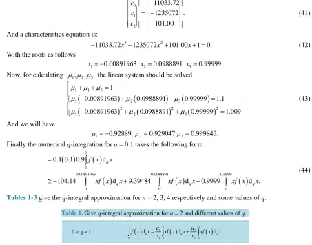
0 1 2

11033.72

1235072 .

101.00

c c c

−

   

  _{= −} 

   

   

(41)

And a characteristics equation is:

3 2

11033.72x 1235072x 101.00x 1 0.

− − + + = (42)

With the roots as follows

1 0.00891963 2 0.0988891 3 0.99999.

x = − x = x =

Now, for calculating µ µ µ₁, ₂, ₃ the linear system should be solved

(

)

(

)

(

)

(

)

(

)

(

)

1 1 3

1 2 3

2 2 2

1 2 3

1

0.00891963 0.0988891 0.99999 1.1 .

0.00891963 0.0988891 0.99999 1.009

µ µ µ

 + + =

 ₋ ₊ ₊ ₌

 

− + + =



(43)

And we will have

1 0.92889 2 0.929047 3 0.999843.

µ = − µ = µ =

Finally the numerical q-integration for q = 0.1 takes the following form

( )

1 0

0.00891963 0.0988891 0.9999

0 0 0

0.1 0.1 0.9 d

104.14 d 9.39484 d 0.9999 d .

q

q q q

f x x

xf x x xf x x xf x x

=

≅ − + +

∫

(44)

[image:6.595.87.541.89.444.2]

Tables 1-3give the q-integral approximation for n = 2, 3, 4 respectively and some values of q.

Table 1. Give q-integral approximation for n = 2 and different values of q.

( ) 1 ( ) 2 ( )

1

1 2

0 10 2 0

d f d d

x x

q q q

f x x x x x xf x x

x x

µ µ

≅ +

∫

0 q 1

( ) ( ) ( )

1 0.425994 0.968283

0 0 0

dq 0.22176 dq 1.13032 dq

f x x≅ − xf x x+ xf x x

∫

q = 0.1

( ) ( ) ( )

1 0.367354 0.940327

0 0 0

dq 0.3323 dq 1.1933 dq

f x x≅ − xf x x+ xf x x

∫

q = 0.2

( ) ( ) ( )

1 0.319002 0.916554

0 0 0

dq 0.972855 dq 1.429637 dq

f x x≅ − xf x x+ xf x x

∫

q = 0.3

( ) ( ) ( )

1 0.198698 0.8902836

0 0

dq 2.35192 dq 1.64814 dq

f x x≅ − xf x x+ xf x x

∫

０ q = 0.4

( ) ( ) ( )

1 0.258459 0.883551

0 0 0

dq 2.08851 dq 1.74273 dq

f x x≅ − xf x x+ xf x x

∫

q = 0.5

( ) ( ) ( )

1 0.236532 0.873087

0 0 0

dq 2.76961 dq 1.89569 dq

f x x≅ − xf x x+ xf x x

∫

q = 0.6

( ) ( ) ( )

1 0.221425 0.866244

0 0 0

dq 3.46192 dq 2.03933 dq

f x x≅ − xf x x+ xf x x

∫

q = 0.7

( ) ( ) ( )

1 0.210175 0.862271

0 0 0

dq 4.16026 dq 2.17378 dq

f x x≅ − xf x x+ xf x x

∫

q = 0.8

( ) ( ) ( )

1 0.20059 0.86045

0 0 0

dq 4.88649 dq 2.30111 dq

f x x≅ − xf x x+ xf x x

∫

(7)

Table 2. Give the q-integral approximation for n = 3 and different values of q.

( ) 1 ( ) 2 ( ) 3 ( )

1

3

1 2

0 1 0 2 0 30

d d d d

x

x x

q q q q

f x x xf x x xf x x xf x x

x x x

µ

µ µ

≅ + +

∫

0 q 1

( ) ( ) ( ) ( )

1 0.00891963 0.0988891 0.9999

0 0 0 0

dq 104.14 dq 9.39484 dq 0.9999 dq

f x x≅ − xf x x+ xf x x+ xf x x

∫

q = 0.1

( ) ( ) ( ) ( )

1 0.0192011 0.182476 0.999892

0 0 0 0

dq 512789 dq 5.34473 dq 0.999815 dq

∫

q = 0.2

( ) ( ) ( ) ( )

1 0.0268083 0.249164 0.999173

0 0 0 0

dq 40.3706 dq 4.33208 dq 1.0037 dq

∫

q = 0.3

( ) ( ) ( ) ( )

1 0.0445189 0.313376 0.997668

0 0 0 0

dq 24.8842 dq 3.50782 dq 1.01091 dq

∫

q = 0.4

( ) ( ) ( ) ( )

1 0.053713 0.357446 0.994861

0 0 0 0

dq 22.2718 dq 3.29942 dq 1.03103 dq

∫

q = 0.5

( ) ( ) ( ) ( )

1 0.0549073 0.37657 0.990456

0 0 0 0

dq 24.1157 dq 3.35099 dq 1.07248 dq

∫

q = 0.6

( ) ( ) ( ) ( )

1 0.0452327 0.631928 0.982296

0 0 0 0

dq 34.2422 dq 3.89172 dq 1.1609 dq

∫

q = 0.7

( ) ( ) ( ) ( )

1 0.0404423 0.165438 0.951337

0 0 0 0

dq 108.109 dq 24.1038 dq 1.4553 dq

∫

q = 0.8

( ) ( ) ( ) ( )

1 0.0484744 0.373827 0.975824

0 0 0 0

dq 37.2967 dq 4.12227 dq 1.2983 dq

∫

[image:7.595.98.539.399.715.2]

q = 0.9

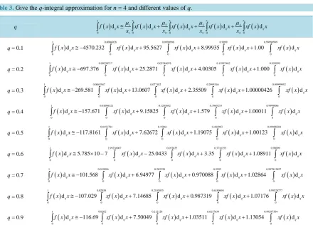
Table 3. Give the q-integral approximation for n = 4 and different values of q.

( ) 1 ( ) 2 ( ) 3 ( ) 4 ( )

1

3

1 2 4

0 10 2 0 3 0 4 0

d d d d d

x

x x x

q q q q q

f x x xf x x xf x x xf x x xf x x

x x x x

µ

µ µ µ

≅ + + +

∫

q

( ) ( ) ( ) ( ) ( )

1 0.0004028 0.0999998 0.9999 0.99999999

0 0 0 0 0

dq 4570.232 dq 95.5627 dq 8.99935 dq 1.00 dq

f x x≅ − xf x x+ xf x x+ xf x x+ xf x x

∫

q = 0.1

( ) ( ) ( ) ( ) ( )

1 0.00250717 0.03748678 0.19997462 0.999999

0 0 0 0 0

dq 697.376 dq 25.2871 dq 4.00305 dq 1.000 dq

∫

q = 0.2

( ) ( ) ( ) ( ) ( )

1 0.0063567 0.077182 0.2995346 0.99999952

0 0 0 0 0

dq 269.581 dq 13.0607 dq 2.35509 dq 1.00000426 dq

∫

q = 0.3

( ) ( ) ( ) ( ) ( )

1 0.01096321 0.1203692 0.3965253 0.9999886

0 0 0 0 0

dq 157.671 dq 9.15825 dq 1.579 dq 1.00011 dq

∫

q = 0.4

( ) ( ) ( ) ( ) ( )

1 0.0151781 0.15861 0.484903 0.99988304

0 0 0 0 0

dq 117.8161 dq 7.62672 dq 1.19075 dq 1.00123 dq

∫

q = 0.5

( ) ( ) ( ) ( ) ( )

1 2.99236007 0.052835 0.3716355 0.98999

0 0 0 0 0

dq 5.785 10 7 dq 25.0433 dq 3.35 dq 1.08911 dq

f x x≅ × − xf x x− xf x x+ xf x x+ xf x x

∫

q = 0.6

( ) ( ) ( ) ( ) ( )

1 0.019896 0.203338 0.5992 0.997813857

0 0 0 0 0

dq 101.568 dq 6.94977 dq 0.970088 dq 1.02864 dq

∫

q = 0.7

( ) ( ) ( ) ( ) ( )

1 0.02038 0.2105035 0.6180694 0.99528777

0 0 0 0 0

dq 107.029 dq 7.14685 dq 0.987319 dq 1.07176 dq

∫

q = 0.8

( ) ( ) ( ) ( ) ( )

1 0.0202 0.212128 0.6217634 0.99297304

0 0 0 0 0

dq 116.69 dq 7.50049 dq 1.03511 dq 1.13054 dq

∫

(8)

[image:8.595.85.539.106.291.2]

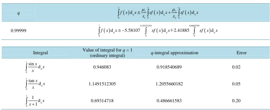
Table 4.Give the q-integral approximation for n = 2 and almost extreme value of q = 0.99999 for three different integrants in a specified interval.

q ( ) ( ) ( )

1 2

1

1 2

0 10 2 0

d d d

x x

q q q

f x x xf x x xf x x

x x

µ µ

≅ +

∫

0.99999 ( ) ( ) ( )

1 0.19371354 0.8603795

0 0 0

dq 5.58107 dq 2.41885 dq

f x x≅ − xf x x xf x x

∫

＋

∫

Integral Value of integral for _{(ordinary integral)}q = 1 q-integral approximation Error

1 0

sin dq

x x x

∫

0.946083 0.918540689 0.02

1 0

tan dq

x x x

∫

1.1491512305 1.2055660182 0.05

1 0

1 d

1 qx

x+

∫

0.69314718 0.486661583 0.20

5. Error Analysis and Application of q-Integral for Integral Approximation

The numerical values show for all values of n the error of q-integrations fluctuate for different values of q, it seems q = 0.70 gives the worse error almost for all values of n, the errors decreases as q approaches to the ex-treme values 0 and 1. Using this result and (3) the q-integral can be calculated for very large value of q ap-proaching to 1 which will approximate the ordinary integrals whose q-integrals is easier than ordinary integrals by using q-integral approximation for n = 2 and different values of q, as illustrated inTable 4 and following the examples, where

( )

1

0 0

lim d d .

z z

q

q→

∫

f x x=

∫

f x x

6. Conclusion

In this paper, a new algorithm for the numerical approximation of q-integration based on q-calculation of appro-priate nodes and weights is introduced. The evaluation of nodes and weight is based on q-integral error minimi-zation, as expected in the numerical examples which give a good approximation in comparison with exact solu-tions for the given values of q and fixed n. As the q-fractional integration can be transferred to q-integrals, the procedure is also applicable for q-fractional integration, and also improper integrals for the large values of q.

References

[1] Rajkovic, P.M., Marinkovic, S.D. and Stankovic, M.S. (2007) Fractional Integrals and Derivatives in q-Calculus. Ap-plicable Analysis and Discrete Mathematics, 1, 311-323. http://dx.doi.org/10.2298/AADM0701311R

[2] Bostan, A., Salvy, B., Chowdhury, M.F.I., Schost, E., Lebreton, R. and Max, E. (2014) Power Series Solution of Sin-gular q-Differential Equations. Journal of Combinatorial Theory, Series A, 121, 45-63.

http://dx.doi.org/10.1016/j.jcta.2013.09.005

[3] Kim, T. (2007) On the Analogs of Euler Number and Polynomials Associated with p-Adic q-Integral on Zp at q = −1.

Journal of Mathematical Analysis and Applications, 331, 779-792. http://dx.doi.org/10.1016/j.jmaa.2006.09.027 [4] Lim, S.C., Eab, C.H., Mak, K.H., Li, M. and Chen, S.Y. (2012) Solving Linear Coupled Fractional Differential

Equa-tions by Direct Operational Method and Some ApplicaEqua-tions. Mathematical Problems in Engineering, 2012, Article ID: 653939. http://dx.doi.org/10.1155/2012/653939

[5] Foupouagnigni, M., Koepf, W. and Ronveaux, A. (2004) On Factorization and Solutions of q-Difference Equations Sa-tisfied by Some Classes of Orthogonal Polynomials. Journal of Computational and Applied Mathematics, 162, 299- 326. http://dx.doi.org/10.1016/j.cam.2003.04.005

(9)

[7] De la Sen, M. (2014) On Nonnegative Solutions of Fractional q-Linear Time-Varying Dynamics. Hindawi Publisher Co. Abstract and Applied Analysis, 2014, Article ID: 247375. http://dx.doi.org/10.1155/2014/247375

[8] Simsek, Y. (2006) q-Dedekind Type Sums Related to q-Zeta Function and Basic L-Series. Journal of Mathematical Analysis and Applications, 318, 333-351. http://dx.doi.org/10.1016/j.jmaa.2005.06.007

[9] Abdeljavad, T., Benli, B. and Baleanu, D. (2012) A Generalized q-Mittag-Leffler Function by q-Captuo Fractional Li-near Equations. Hindawi Publisher Co. Abstract and Applied Analysis, 2012, Article ID: 546062.

[10] Ismail, M.E.H. and Stanton, D. (2003) q-Taylor Theorems, Polynomial Expansions and Interpolation of Entire Func-tions. Journal of Approximation Theory, 123, 125-146. http://dx.doi.org/10.1016/S0021-9045(03)00076-5

[11] Stankovic, M.S., Rajkovic, P.M. and Marinkovic, S.D. (2006) Inequalities Which Includes q-Integrals. Bulletin: Classe des sciences mathematiques et natturalles, 133, 137-146.

[12] Wu, G.-C. and Baleanu, D. (2013) New Application of the Variation Iteration Method from Differential Equation to q-Fractional Difference Equations. Advanced in Difference Equation, 21.

[13] Hashemiparast, S.M. (2011) Numerical Solution of the Integrals by Using Appropriate Nodes and Weights. Proceed-ings of theICMS Conference, Istanbul.

[14] Ernst, T. (2003) A Method for q-Calculus. Journal of Nonlinear Mathematical Physics, 10, 487-525. http://dx.doi.org/10.2991/jnmp.2003.10.4.5

[15] Jackson, F.H. (1910) On q-Definite Integrals. Quarterly Journal of Pure and Applied Mathematics, 41, 193-203. [16] Koekoek, R., Alesky, P. and Swarrouw, R. (2010) Hyper Geometric Orthogonal Polynomials and Their q-Analogues.

Cambridge University Press, Cambridge.

[17] Miao, Y. and Feng, Q. (2009) Several q-Integrals Inequalities. Journal of Mathematical Inequalities, 3, 115-121. http://dx.doi.org/10.7153/jmi-03-11

[18] Hashemiparast, S.M., Eslahchi, M.R. and Dehghan, M. (2007) Determination of Nodes in Numerical Integration Rules Using Difference Equations. Applied Mathematics and Computation, 176, 117-122.

[19] Rietsch, K. (2001) Totally Positive Toeplitz Matrices and Quantum Cohomology of Partial Flag Varieties. Journal of the American Mathematics Society, 16, 363-392.

[20] Andersen, J.E. and Berg, C. (2009) Quantum Hilbert Matrices and Orthogonal Polynomials. Journal of Computational and Applied Mathematics, 233, 723-729.

[22] Gray, R.M. (2006) Toeplitz and Circulant Matrices: A Review. Department of Electrical Engineering, Stanford Uni-versity, Stanford.