Physically Inspired Models for the Synthesis of Stiff Strings with Dispersive Waveguides

(1)

Physically Inspired Models for the Synthesis of Stiff

Strings with Dispersive Waveguides

I. Testa

Dipartimento di Scienze Fisiche, Universit`a di Napoli “Federico II,” Complesso Universitario di Monte S. Angelo, 80126 Napoli, Italy Email:[email protected]

G. Evangelista

S. Cavaliere

Received 30 June 2003; Revised 17 November 2003

We review the derivation and design of digital waveguides from physical models of stiffsystems, useful for the synthesis of sounds from strings, rods, and similar objects. A transform method approach is proposed to solve the classic fourth-order equations of stiffsystems in order to reduce it to two second-order equations. By introducing scattering boundary matrices, the eigenfrequencies are determined and theirn2 _{dependency is discussed for the clamped, hinged, and intermediate cases.} On the basis of the frequency-domain physical model, the numerical discretization is carried out, showing how the insertion of an all-pass delay line generalizes the Karplus-Strong algorithm for the synthesis of ideally flexible vibrating strings. Know-ing the physical parameters, the synthesis can proceed usKnow-ing the generalized structure. Another point of view is offered by Laguerre expansions and frequency warping, which are introduced in order to show that a stiffsystem can be treated as a nonstiffone, provided that the solutions are warped. A method to compute the all-pass chain coefficients and the optimum warping curves from sound samples is discussed. Once the optimum warping characteristic is found, the length of the dis-persive delay line to be employed in the simulation is simply determined from the requirement of matching the desired fun-damental frequency. The regularization of the dispersion curves by means of optimum unwarping is experimentally evalu-ated.

Keywords and phrases:physical models, dispersive waveguides, frequency warping.

1. INTRODUCTION

Interest in digital audio synthesis techniques has been rein-forced by the possibility of transmitting signals to a wider au-dience within the structured audio paradigm, in which algo-rithms and restricted sets of data are exchanged [1]. Among these techniques, the physically inspired models play a privi-leged role since the data are directly related to physical quan-tities and can be easily and intuitively manipulated in order to obtain realistic sounds in a flexible framework. Applica-tions are, amongst the others, the simulation of a “physical situation” producing a class of sounds as, for example, a clos-ing door, a car crash, the hiss made by a crawlclos-ing creature, the human-computer interaction and, of course, the simulation of musical instruments.

In the general physical models technique, continuous-time solutions of the equations describing the physical

(2)

In the following, we will focus on stiffvibrating systems, including rods and stiff strings as encountered in pianos. However, extensions to two- or three-dimensional systems can be carried out with little effort.

Vibrating physical systems have been extensively studied over the last thirty years for their key role in many musi-cal instruments. The wave equation can be directly approxi-mated by means of finite difference equations [3,4,5,6,7], or by discretization of the wave functions as proposed by Jaffe and Smith [8,9] who reinterpreted and generalized the Karplus-Strong algorithm [10] in a wave propagation setting. The outcome of the approximation of the time domain solu-tion of the wave equasolu-tion is the design of a digital waveg-uide simulating the string itself: the sound signal simulation is achieved by means of an appropriate excitation signal, such as white noise. However, in order to achieve a more realistic and flexible synthesis, the interaction of the excitation sys-tem with the vibrating element is, in turn, physically mod-eled. Digital waveguide methods for the simulation of physi-cal models have been widely used [11,12,13,14,15,16]. One of the reasons for their success is that they are appropriate for real-time synthesis [17,18,19,20]. This result allowed us to change our approach to model musical instruments based on vibrating strings: waveguides can be designed for modeling the “core” of the instruments, that is, the vibrating string, but they are also suitable for the integration of interaction mod-els, for example, for the excitation due to a hammer [21] or to a bow [9], the radiation of sound due to the body of the instrument [22,23,24,25], and of different side-effects in plucked strings [26]. It must be pointed out that the interac-tions being highly nonlinear, their modeling and the deter-mination of the range of stability is not an easy task.

In this paper, we will review the design of a digital waveg-uide simulating a vibrating stiff system, focusing on stiff strings and treating bars as a limit case where the tension in negligible. The purpose is to derive a general framework inspiring the determination of a discrete numerical model. A frequency domain approach has been privileged, which allows us to separate the fourth-order differential equation of stiffsystems into two second-order equations, as shown in Section 2. This approach is also useful for the simula-tion of two-dimensional (2D) systems such as thin plates. By enforcing proper boundary conditions, we obtain the eigenfrequencies and the eigenfunctions of the system as found, for the case of strings, in the classic works by Fletcher [27, 28]. Once the exact solutions are completely charac-terized, their numerical approximation is discussed [29,30] together with their justification based on physical reason-ing. The discretization of the continuous-time domain so-lutions is carried out in Section 3, which naturally leads to dispersive waveguides based on a long chain of all-pass fil-ters. From a different point of view, the derived structure can be described in terms of Laguerre expansions and frequency warping [31]. In this framework, a stiffsystem can be shown to be equivalent to a nonstiff(Karplus-Strong like) system, whose solutions are frequency warped, provided that the ini-tial and the possibly moving boundary conditions are prop-erly unwarped [32,33]. As a side effect, this property can be

exploited in order to perform an analysis of piano sounds by means of pitch-synchronous frequency warped wavelets in which the excitation can be separated from the resonant sound components [34].

The models presented in this paper provide at least two entry points for the synthesis. If the physical parameters and boundary conditions are completely known, or if it is de-sired to specify them to model arbitrary strings or rods, then the eigenfunctions, hence the dispersion curve, can be deter-mined. The problem is then reconducted to that of finding the best approximation of the continuous-time dispersion curve with the phase response of a suitable all-pass chain us-ing the methods illustrated inSection 3. Another entry point is oﬀered if sound samples of an instrument are available. In this case, the parameters of the synthesis model can be determined by finding the warping curve that best fits the data given by the frequencies of the partials, together with the length of the dispersive delay line. This is achieved by means of a regularization method of the experimental dis-persion data, as reported inSection 4.

The physical entry point is to be preferred in those sit-uations where sound samples are not available, for example, when we are modeling a nonexisting instrument by extension of the physical model, such as a piano with unusual speak-ing length. The other entry level is best for approximatspeak-ing real instrument sounds. However, in this case, the synthesis is limited to existing sources, although some variations can be obtained in terms of the warping parameters, which are related to, but do not directly represent, physical factors.

2. PHYSICAL STIFF SYSTEMS

In this section, we present a brief overview of the stiﬀ string and rod equations of motion and of their solution. The purpose is twofold. On the one hand, these equations give the necessary background to the physical modeling of stiﬀ strings. On the other hand, we show that their fre-quency domain solution ultimately provides the link between continuous-time and discrete-time models, useful for the derivation of the digital waveguide and suitable for their sim-ulation. This link naturally leads to Laguerre expansions for the solution and to frequency warping equivalences. Further-more, enforcing proper boundary conditions determines the eigenfrequencies and eigenfunctions of the system, useful for fitting experimentally measured resonant modes to the ones obtained by simulation. This fit allows us to determine the parameters of the waveguide through optimization.

2.1. Stiff string and bar equation

The equation of motion for the stiﬀstring can be determined by studying the equilibrium of a thin plate [35,36]. One ob-tains the following 4th-order diﬀerential equation for the de-formation of the stringy(x,t):

−ε∂4y(x,t) ∂x4 +

∂2_y₍_x_,_t₎ ∂x2 =

1

c2

∂2_y₍_x_,_t₎ ∂t2 ,

ε=EI

T, c=

T ρS,

(3)

featuring the Young modulus of the materialE, the inertia moment I with respect to the transversal axis of the cross-section of the string (for a circular cross-section of radiusr,I = πr4_/_{4 as in [}₃₆_{]), the tension of the string}_T_{, and the mass}

per unit lengthρS. Note that forε→0, (1) becomes the well-known equation of the vibrating string [35]. Otherwise, if the applied tensionTis negligible, we obtain

−ε∂4y(x,t)

which is the equation for the transversal vibrations of rods. Solutions of (1) and (2) are best found in terms of the Fourier transform ofy(x,t) with respect to time:

Y(x,ω)= +∞

−∞ y(x,t) exp(−iωt)dt, (3)

whereωis the angular velocity related to frequencyf by the relationship f =2πω.

By taking the Fourier transform of both members of (1) and (2), we obtain

for the stiﬀstring and

ε∂

4_Y₍_x_,_ω₎

∂x4 −ω

2_Y₍_x_,_ω₎₌₀ ₍₅₎

for the rod.

The second-order−∂2_/∂x2_{spatial di}_ﬀ_{erential operator is}

defined as a repeated application of theL2space extension of

the−i(∂/∂x) operator [37]. To the purpose, we seek solutions whose spatial and frequency dependency can be factored, ac-cording to the separation of variables method, as follows:

Y(x,ω)=W(ω)X(x). (6)

Substituting (6) in (4) and (5) results in the elimination of the W(ω) term, obtaining ordinary diﬀerential equations, whose characteristic equations, respectively, are

ελ4−λ2−ω2

c2 =0 (stiﬀstring), ελ4−ω2=0 (rod).

(7)

The elementary solutions for the spatial partX(x) have the formX(x)=Cexp(λx). It is important to note that in both cases, the characteristics equations have the following form:

whereξ1 andξ2 are, in general, complex numbers that

de-pend onω. Equation (8) allows us to factor both equations in (4) and (5) as follows:

The operator −∂2_/∂x2 _{is selfadjoint with respect to the}_L 2

scalar product [37]. Therefore, (9) can be separated into the following twoindependentequations:

As we will see, (10) justifies the use, with proper modifica-tions, of a second-order generalized waveguide based on pro-gressive and repro-gressive waves for the numerical simulation of stiﬀsystems.

2.2. General solution of the stiff string and bar equations

In this section, we will provide the general solution of (8). The particular eigenfunctions and eigenfrequencies of rods and stiﬀstrings are determined by proper boundary condi-tions and are treated inSection 2.3. From (7), it can be shown

Note that in both cases, the eigenvaluesξ1±are complex

num-bers, whileξ2±are real numbers. It is also worth noting that

ξ2

where ξ1 corresponds to the positive choice of the sign in

front of the square root in (12) andξ2= |ξ2±|. As expected, if

we letT →0, then both sets of eigenvalues of the stiﬀstring tend to those found for the rod. Using the equations in (12), we then have for both strings and rods

Y1(x,ω)=c+1exp

(4)

From (12), we see that the primary eﬀect of stiﬀness is the dependency on frequency of the argument (from now on,

phase) of the solutions of (4) and (5). Therefore, the propa-gation of the wave from one section of the string located atx

to the adjacent section located atx+∆xis obtained by multi-plication of a frequency dependent factor exp(ξ1∆x).

Conse-quently, the group velocityu, defined asu≡(dξ1/dω)−1, also

depends on frequency. This results in a dispersion of the wave packet, characterized by the functionξ1(ω), whose modulus

is plotted inFigure 1for the case of a brass string using the following values of the physical parametersr,T,ρ, andE:

Clearly, the previous example is a very crude approximation of a physical piano string (e.g., real-life piano strings in the low register are built out of more than one material and a copper or brass wire is wrapped around a steel core). For the sake of completeness, we give the explicit expression of|u|in both the cases we are studying. We have

|u| = 2c

IfT →0, the two group velocities are equal. Moreover, if in the first line in (16), we letε→0, thenu→c, which is the limit case of the ideally flexible vibrating string. These facts further justify the use of a dispersive waveguide in the nu-merical simulation. With respect to this point, a remark is in order: the dispersion introduced by stiﬀness can be treated as a limiting “nonphysical” consequence of the Euler-Bernoulli beam equation:

wherepis the distributed load acting on the beam. It is “non-physical” in the sense that u → ∞as√ω. However, in the discrete-time domain, this “nonphysical” situation is avoided if we suppose all the signals be bandlimited.

2.3. Complete characterization of stiff string and rod solution

Boundary conditions for real piano strings lie in between the conditions of clamped extrema:

Y

Figure1: Plot of the phase module of the stiﬀmodel equation so-lution forε=π/4 cm2_and_c_≈₂_∗₁₀4_{cm s}−1_.

Before determining the conditions for the eigenfrequencies of the considered stiﬀsystems, we find a more compact way of writing (18) and (19). Starting from the factorized form of the stiﬀsystems equation (see (10)), and using the symbols introduced inSection 2.2, we have

Y1(x,ω)=ψ1+(x,ω) +ψ1−(x,ω),

Conditions (18) can then be rewritten as follows:

Y1

At the terminations of the string or of the rod, we have

(5)

which can be rewritten in matrix form:

By left-multiplying both members of (24) for the inverse of the_ξ1 1+

The matrix Sc relates the incident wave with the reflected wave at the boundaries. Independently of the rootsξi, it has the following properties:

which, in matrix form, becomes

TheSh matrix for the hinged stiﬀsystem is independent of rootsξi. The matricesSh andScare related in the following way:

_Sh_{= −}_Sc_, S2

h=S2c.

(32)

In conclusion, the boundary conditions for stiffsystems can be expressed in terms of matrices that can be used in the numerical simulation of stiffsystems. Moreover, since the real-life boundary conditions for stiffstrings in piano lie in

between the conditions given in (18) and (19), we can com-bine the two matrices Sc andSh in order to enforce more general conditions, as illustrated inSection 3. In the follow-ing, we will solve (4) and (5) applying separately these sets of boundary conditions.

2.3.1. The clamped stiff string and rod

In order to characterize the eigenfunctions in the case of con-ditions (18), in (12) we let

ξ1=iξ1 (33)

for both the stiﬀstring and the rod solution. By definition,

ξ1is a real number. Moreover, for the rod, we haveξ1 =ξ2.

With this position, it can be shown that conditions (18) for the stiﬀstring lead to the equations [35,38]

while, for the rod, we have

cosξ1L

coshξ2L

=1. (35)

Equations (34) and (35) can be solved numerically. In partic-ular, taking into account the second line in (12), solutions of (35) are [35]

A similar trend can be obtained for the stiﬀstring. In view of their historical and practical relevance, we here report the numerical approximation for the allowed eigenfrequencies of the stiﬀstring given by Fletcher [27]:

If we expand the above expression in a series of powers of

αtruncated to second order, we have the following approxi-mate formula valid for small values of stiﬀness:

ωn

The last approximation does not apply to bars. Forε=0, we haveα=0 and the eigenfrequencies tend to the well-known formula for the vibrating string [35]:

ωn=nω1. (39)

(6)

r=3 mm

r=1 mm

0 10 20 30 40

Partial number 0

1 2 3 4 5 6 7 8 9

R

elati

ve

spacing

Figure 2: Typical eigenfrequencies relative spacing curves of the clamped stiﬀstring for diﬀerent values of the radiusrof the sec-tionS.

shown inFigure 2with variabler, where values of the other physical parameters are the same as in (15).

Due to the dependency on the frequency of the phase of the solution, the eigenfrequencies of the stiffstring are not equally spaced. For a small radius r, hence for low degree of the stiffness of the string (see (1)), the relative spacing is almost constant for all the considered order of eigenfrequen-cies. However, for higher stiffness, the spacing of the eigen-frequencies increases, in first approximation, as a linear func-tion of the order of the eigenfrequency. The above results are summarized by the typical “warping curves” of the system, shown inFigure 3, in which the quantityωn−ωn, which rep-resents the deviation from the linearity, is plotted in terms of spacing∆ωnbetween consecutive eigenfrequencies.

In the stiﬀstring case, we have two sets of eigenfunctions, one having even parity and the other one having odd parity, whose analytical expressions are respectively given by [38]

Y(x,ω)=C(ω) cos

ξ1L₂

cosξ1x

cosξ1(L/2)

− cosh

ξ2x

coshξ2(L/2)

,

Y(x,ω)=C(ω) sin

ξ1L₂

sinξ1x

sinξ1(L/2)

− sinh

ξ2x

sinhξ2(L/2)

,

(40)

whereC(ω) is a constant that can be calculated imposing the initial conditions.

2.3.2. Hinged stiff string and rod

Conditions (19) lead to the following sets of equations for the stiﬀstring:

sinξ1L

sinhξ2L

=0,

ξ1 2

+ξ2 2 =0,

(41)

r=3 mm

r=1 mm

0 500 1000 1500 2000

Frequency (Hz) 0

500 1000 1500 2000 2500 3000 3500

De

vi

ation

fr

o

m

linear

it

y

(Hz)

Figure3: Typical warping curves of the clamped stiﬀstring for dif-ferent values of the radiusrof the sectionS.

and for the rod:

sinξ1L

sinhξ2L

=0. (42)

The second line in (41) has no solutions since bothξ12and ξ2

2 are real functions. It follows that hinged stiﬀsystems are

only described by (42). In this equation, sinh(ξ2L) =0 has

no solution, hence the eigenfrequencies are determined by the condition

ξ1= nπ

L . (43)

Using the parameters αandαrespectively defined in (36) and (37), the eigenfrequencies for the hinged stiﬀstring are

exactlyexpressed as follows:

ωn=

nπc L

n2_π2_α2_{+ 1}_, ₍₄₄₎

while for the rod, we have

ωn=n2_π2_α2_. ₍₄₅₎

As the tension T → 0, (44) tends to (45). Figure 4shows the relative spacing of the eigenfrequencies in the case of the hinged stiﬀstring.

Relative eigenfrequencies spacing curves are very similar to the ones of the clamped string and so are the “warping curves” of the system, as shown inFigure 5.

Using (45), we can give an analytic expression for the rel-ative spacing of the eigenfrequencies of the hinged rod. We have

π2_α2₍₂_n_{+ 1)}_. ₍₄₆₎

(7)

r=3 mm

r=1 mm

0 10 20 30 40

Partial number 0

2 4 6 8 10

R

elati

ve

spacing

Figure 4: Typical eigenfrequencies relative spacing curves of the hinged stiﬀstring for diﬀerent values of the radiusrof the section

S.

r=3 mm

r=1 mm

0 500 1000 1500 2000

Frequency (Hz) 0

500 1000 1500 2000 2500 3000 3500 4000

De

vi

ation

fr

o

m

linear

it

y

(Hz)

Figure5: Typical warping curves of the hinged stiﬀstring for dif-ferent values of the radiusrof the sectionS.

eigenfunctions for the stiﬀstring [38]:

Yn(x,ω)=2D(ω) sin

2nπ L x

,

Yn(x,ω)=2D(ω) cos

(2n+ 1)π

L x

,

(47)

whereD(ω) must be determined by enforcing the initial con-ditions. It is worth noting that both functions in (47) are in-dependent of the stiﬀness parameterε. InSection 3, we will use the obtained results in order to implement the dispersive waveguides digitally simulating the solutions of (4) and (5).

Finally, we need to stress the fact that the eigenfrequen-cies of the hinged stiﬀstring are similar to the ones for the clamped case except for the factor (1 + 2α+ 4α2_{). Therefore,}

for small values of stiﬀness, they do not diﬀer too much. This

X(z) 2Pdelays Y(z)

z−2P

G(z) (low-pass)

Figure6: Basic Karplus-Strong delays cascade.

can also be seen from the similarity of the warping curves ob-tained with the two types of boundary conditions.

Taking into account the fact that real-piano strings boundary conditions lie in between these two cases, we can conclude that the eigenfrequencies of real-piano strings can be calculated by means of the approximated formula [27,28]:

ωnAnBn2_{+ 1,} ₍₄₈₎

whereAandBcan be obtained from measurements. Approx-imation (48) is useful in order to match measured vibrating modes against the model eigenfrequencies.

3. NUMERICAL APPROXIMATIONS OF STIFF SYSTEMS

Most of the problems encountered when dealing with the continuous-time equation of the stiﬀstring consist in de-termining the general solution and in relating the initial and boundary conditions to the integrating constants of the equation. In this section, we will show that we can use a sim-ilar technique also in discrete-time, which yields a numerical transform method for the computation of the solution.

InSection 2, we noted that (1) becomes the equation of vibrating string in the case of negligible stiﬀness coeﬃcientε. It is well known that the technique known as Karplus-Strong algorithm implements the discrete-time domain solution of the vibrating string equation [8], allowing us to reach good quality acoustic results. The block diagram of the adopted loop circuit is shown inFigure 6.

The transfer function of the digital loop chain can be written as follows:

H(z)= 1

1−z−2P_G₍_z₎, (49)

where the loop filter G(z) takes into account losses due to nonrigid terminations and to internal friction, andP is the number ofsectionsin which the string is subdivided, as ob-tained from time and space sampling. Loop filters design can be based on measured partial amplitude and frequency trajectories [18], or on linear predictive coding (LPC)-type methods [9]. The filterG(z) can be modelled as IIR or FIR and it must be estimated from samples of the sound or from a model of the string losses, where, for stability, we need

|G(ejω₎_|_<_{1. Clearly, in the IIR case or in the nonlinear phase}

(8)

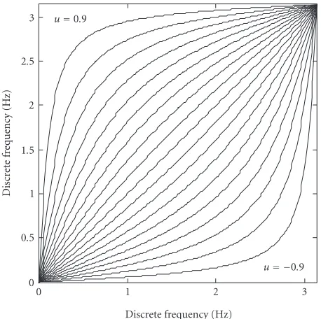
u=0.9

u= −0.9

0 1 2 3

Discrete frequency (Hz) 0

0.5 1 1.5 2 2.5 3

Discr

et

e

fr

equency

(Hz)

Figure7: First-order all-pass phase plotted for various values ofu.

limited amount of dispersion. Additional phase terms in the form of all-pass filters can be added in order to tune the string model to the required pitch [13] and contribute to fur-ther dispersion.

Since the group velocity for a traveling wave for a stiﬀ sys-tem depends on frequency (see (16)), it is natural to substi-tute, in discrete time, the cascade of unit delays with a chain of circuital elements whose phase responses do depend on frequency. One can show that the only choice that leads to rational transfer functions is given by a chain of first-order

all-passfilters [39,40]. More complex physical systems, for example, as in the simulation of a monaural room, call for substituting the delays chain with a more general filter as il-lustrated in [41]:

A(z,u)= z−1−u

1−uz−1 (50)

whose phase characteristic is

θ(Ω)=Ω+ 2 arctan usin(Ω)

1−ucos(Ω). (51)

The phase characteristics in (51) are plotted inFigure 7for various values ofu.

A comparison between the curve inFigure 1and the ones inFigure 7gives more elements of plausibility for the approx-imation of the solution phase of the stiﬀmodel equations, given in (12), with the all-pass filter phase (51). Adopting a similar circuital scheme as in the Karplus-String algorithm [10] in which the unit delays are replaced by first-order all-pass filters, the approximation is given by

ξ1

ΩfsP

Lθ(Ω), (52)

X(z) 2Pall-pass cascade Y(z)

A(z)2P

G(z) (low-pass)

Figure8: Dispersive waveguide used to simulate dispersive systems.

where fsis the sampling frequency. Note that, by definition, both members of (52) are real numbers. Therefore, in thez -domain, a nonstiﬀsystem can be mapped into a stiﬀsystem by means of the frequency warping map

z−1_−→_A₍_z₎_. ₍₅₃₎

The resulting circuit is shown inFigure 8. Note, that the feed-back all-pass chain results in delay-free loops. Computation-ally, these loops can be resolved by the methods illustrated in [34,42,43]. Moreover, the phase response of the loop filter

G(z) contributes to the dispersion and it must be taken into account in the global model.

The circuit inFigure 8can be optimized in order to take into account the losses and the coupling amongst strings (e.g., as in piano). In the framework of this paper, we con-fined our interest to the design of the stiﬀsystem filter. For a review of the design of lossy filters and coupling models, see [17].

3.1. Stiff system filter parameters determination

Within the framework of the approximation (52) in the case of dispersive waveguide, the integer parameterPcan be ob-tained by constraining the two functions to attain the same values at the extrema of the bandwidth. Sinceθ(π)=π, we have

P=ξ1

π fsL

π . (54)

As we will see, condition (54) is not the only one that can be obtained for the parameterP. The deviation from linearity introduced by the warpingθ(Ω) can be written as follows:

∆(Ω)≡θ(Ω)−Ω=2 arctan usin(Ω)

1−ucos(Ω). (55)

The function ∆(Ω) is plotted, for diﬀerent values ofu, in Figure 9.

One can see that the absolute value of∆(Ω) has a max-imum which corresponds to the maxmax-imum deviation from the linearity ofθ(Ω). It can be shown that this maximum oc-curs for

(9)

u=0.9

u= −0.9

0 1 2 3

Discrete frequency (Hz) −3

−2 −1 0 1 2 3

De

vi

ation

fr

o

m

linear

it

y

(Hz)

Figure9: Plot of the deviation from linearity of the all-pass filter phase for diﬀerent values of parameteru.

for which the maximum deviation is

∆ΩM,u=2 arcsin(u). (57)

Substituting (56) in (51), we have

θΩM= π

2+ arcsin(u). (58)

Since the solution phaseξ1is approximated byθ(Ω), it has to

satisfy the condition

ξ1

_ΩM

T

L

P

π

2 + arcsin(u) (59)

and therefore, we have the following bound onP:

PLξ1

fsarccos(u)

π/2 + arcsin(u) . (60)

For higher-orderQall-pass filters, (60) can be written as fol-lows:

P 1 Q

Q

i=1 ξ1

fsarccosuiL

π/2 + arcsinui . (61)

An optimization algorithm can be used to obtain the vector parameter u. Based on our experiments, we estimated that an optimal orderQis 4 for the piano string. Therefore, us-ing the values in (15) for the 58 Hz tone of anL =200 cm brass string, we obtainP=209. Although this is not a model for a real-life wound inhomogeneous piano string, this ex-ample gives a rough idea of the typical number of the re-quired pass sections. The computation of this long all-pass chain can be too heavy for real-time applications.

There-fore, an approximation of the chain by means of a cascade of an all-pass of order much smaller than 2Pwith unit delays is usually sought [13,29,30]. A simple and accurate approach is to model the all-pass as a cascade of first-order sections with variable real parameter u[38]. However, a more gen-eral approach calls for including in the design second-order all-pass sections, equivalent to a pair of complex conjugated first-order sections [29]. InSection 4, we will bypass this esti-mation procedure based on the theoretical eigenfunctions of the string to estimate the all-pass parameters and the number of sections from samples of the piano.

3.2. Laguerre sequences

An invertible and orthogonal transform, which is related to the all-pass chain included in the stiﬀstring model, is given by the Laguerre transform [44,45]. The Laguerre sequences

li[m,u] are best defined in thez-domain as follows:

Li(z,u)= √

1−u2

1−uz−1

z−1₋_u

1−uz−1 i

. (62)

Thus, the Laguerre sequences can be obtained from the z -domain recurrence

L0(z,u)= √

1−u2

1−uz−1, Li+1(z,u)=A(z)Li(z,u),

(63)

whereA(z) is defined as in (50). Comparison of (62) with (50) shows that the phase of theztransform of the Laguerre sequences is suitable for approximating the phase of the solu-tion of the stiﬀmodel equation. A biorthogonal generaliza-tion of the Laguerre sequences calling for a variableufrom

section tosectionis illustrated in [46]. This is linked to the refined approximation of the solution previously shown.

3.3. Initial conditions

Putting together the results obtained in Section 1, we can write the solution phase of the stiﬀmodelY(Ω,x) as follows (see (11) and (14)):

Y(ω,x)=c+1(ω) exp

iξ1x

+c−1(ω) exp

−iξ1x

. (64)

We are now disregarding the transient term due toξ2since it

does not influence the acoustic frequencies of the system. In discrete time and space, we letx=m(L/P) as in [10]. With the approximation (52), (64) becomes

Y(m,Ω)c+ 1(Ω) exp

imθ(Ω)+c−1(Ω) exp

−imθ(Ω).

(65) Substituting (63) in (65), we have

Y(Ω,m)c+ 1(Ω)Lm

(Ω,u)

L0(z,u)

+c−1(Ω)L

−m(Ω,u) L0(z,u)

, (66)

where we have used the fact that

AeiΩ_,_u₌ e−iΩ−u

1−ue−iΩ =exp

(10)

By defining

V+(Ω)≡ c + 1(Ω) L0(z,u)

, V−(Ω)≡ c −

1(Ω) L0(z,u)

, (68)

(66) can be written as follows:

Y(m,Ω)V+(Ω)Lm(Ω,u) +V−(Ω)L−m(Ω,u). (69)

Taking the inverse discrete-time Fourier transform (IDTFT) on both sides of (69), we obtain

y[m,n]y+[m,n] +y−[m,n], (70)

where

y+[m,n]=

∞

k=−∞

v+[n−k]lm[k,u],

y−[m,n]= ∞

k=−∞

v−[n−k]l−m[k,u],

(71)

and the sequencesv±(n) are the IDTFT ofV±(Ω). For the sake of conciseness, we do not report here the expression of

v±[n] in terms of constantsc1±. For further details, see [31,

38]. The expression of the numerical solutiony[m,n] can be written in terms of a generic initial condition

y[m, 0]=y+[m, 0] +y−[m, 0]. (72)

In order to do this, we resort to the extension of Laguerre sequences to negative arguments:

lm[n,u]=

  lm

[n,u], n≥0,

lm[−n,u], n <0, (73)

and to the property

lm[n,u]=ln[m,−u]. (74)

If we introduce the quantity

y±k[u]= ∞

m=0

y±[m, 0]lk[±m,u],

l_k[±m,u]=l±m[k,u],

(75)

with a simple mathematical manipulation, (71) can be writ-ten as follows:

y+[m,n]=

∞

k=−∞

y+k[u]lm[k+n,u],

y−[m,n]= ∞

k=−∞

y−k[u]lm[k+n,u].

(76)

Therefore, the numeric solution becomes

y[m,n]= ∞

k=−∞

y+klm[k+n,u] + ∞

k=−∞

y−klm[k+n,u]. (77)

We have just shown that the solution of the discrete-time stiffmodel equation can be written as a Laguerre expansion of the initial condition. At the same time, this shows that the stiffstring model is equivalent to a nonstiffstring model cas-caded by frequency warping obtained by Laguerre expansion.

3.4. Boundary conditions

InSection 1, we discussed the stiﬀmodel equation bound-ary conditions in continuous time (see (18) and (19)). In this section, we will discuss the homogenous boundary con-ditions (i.e., the first line in both (18) and (19)) in the discrete-time domain. Using approximation (52) and letting the number ofsectionsof the stiﬀsystemPbe an even integer, we can write the homogenous conditions as follows (see also (69)):

Y

−P

2,Ω

=0

=⇒V+(Ω)L−P/2(Ω,u) +V−(Ω)LP/2(Ω,u)=0,

Y

+P 2,Ω

=0

=⇒V+(Ω)LP/2(Ω,u) +V−(Ω)L−P/2(Ω,u)=0.

(78)

Like (34), (78) can be expressed in matrix form:

LP/2(Ω,u) L−P/2(Ω,u) L−P/2(Ω,u) LP/2(Ω,u)

V+(Ω) V−(Ω)

=

0 0

. (79)

As shown inSection 3.3, the functionsV±(Ω) are determined by means of Laguerre expansion of the initial conditions se-quences through (71) and (76). For any choice of these initial conditions, the determinant of the coeﬃcients matrix in (79) must be zero, obtaining the following condition:

LP/2(Ω,u) 2

−L−P/2(Ω,u)]2=0. (80)

Recalling the z-transform expression for the Laguerre se-quences, we have

sinθ(Ω)P=0, θ(Ω)=kπ

P , k=1, 2, 3,. . . . (81)

In the stiffstring case, the eigenfrequencies of the system are not harmonically related. In our approximation of the phase of the solution with the digital all-pass phase, the harmonic-ity is reobtained at a different level: the displacement of the all-pass phase values is harmonic according to the law writ-ten in (81). The distance between two consecutive values of this phase isπ/P. Due to the nonrigid terminations, the real-life boundary conditions can be given in terms of frequency dependent functions, which are included in the loop filter. In mapping the stiffstructure to a nonstiffone, care must be taken into unwarping the loop filter as well.

4. SYNTHESIS OF SOUND

(11)

0 5 10 15 20 25 30 Partial number

0.2 0.3 0.4 0.5 0.6 0.7

W

ar

ping

par

amet

er

Figure10: Computed all-pass optimized parametersu.

dispersive waveguide, that is, the number of all-pass sections and the coefficientsuiof the all-pass filters. This task could be performed by means of lengthy measurements or estimation of the physical variables, such as tension, Young’s module, density, and so forth. However, as we already remarked, due to the constitutive complexity of the real-life piano strings and terminations, this task seems to be quite difficult and to lead to inaccurate results. In fact, the given physical model only approximately matches the real situation. Indeed, in order to model and justify the measured eigenfrequencies, we resorted to Fletcher’s experimental model described by (48). However, in that case, we ignore the exact form of the eigenfunctions, which is required in order to determine the number of sections of the waveguide and the other param-eters. A more pragmatic and effective approach is to esti-mate the waveguide parameters directly from the measured eigenfrequencies ωn. These can be extracted, for example, from recorded samples of notes played by the piano under exam. Fletcher’s parameters A andB can be calculated as follows:

A= 1

2n

16ω2 n−ω22n

3 ,

B= 1 n2

4γ2₋₁

1−16γ2, γ= ωn ω2n.

(82)

In practice, in the model where the all-pass parameters

ui are equal throughout the delay line, one does not even need to estimate Fletcher’s parameters. In fact, in view of the equivalence of the stiffstring model with the warped non-stiffmodel, one can directly determine, through optimiza-tion, the parameteruthat makes the dispersion curve of the eigenfrequencies the closest to a straight line, using a suitable distance. A result of this optimization is shown inFigure 10. It must be pointed out that our point of view differs from the one proposed in [29,30], where the objective is the

min-0 20 40 60 80

Partial number 20

40 60 80 100 120 140 160 180

Spacing

of

the

p

ar

tials

(Hz)

Figure11: Warped deviation from linearity.

0 10 20 30 40 50

Partial number 0.016

0.017 0.018 0.019 0.02 0.021 0.022

N

o

rmaliz

ed

fr

eq

ue

ncy

Figure12: Optimized all-pass parametersufor A#3 tone.

imization of the number of nontrivial all-pass sections in the cascade.

(12)

0 10 20 30 40 Partial number

0 50 100 150 200 250

Fre

q

u

en

cy

(H

z)

Figure13: Optimum unwarped regularized dispersion curves.

dispersion introduced by the nonisotropic spatial sampling [50]. Since the required warping curves do not match the first-order all-pass phase characteristic, in order to overcome this diﬃculty, a technique including resampling operators has been used in [50, 51] according to a scheme first in-troduced in [33] and further developed in [52] for the wavelet transforms. However, the downsampling operators inevitably introduce aliasing. While in the context of wavelet transforms, this problem is tackled with multichannel filter banks, this is not the case of 2D waveguide meshes.

5. CONCLUSIONS

In order to support the design and use of digital dispersive waveguides, we reviewed the physical model of stiffsystems, using a frequency domain approach in both continuous and discrete time. We showed that, for dispersive propagation in the discrete-time, the Laguerre transform allows us to write the solution of the stiffmodel equation in terms of an or-thogonal expansion of the initial conditions and to reob-tain harmonicity at the level of the displacement of the all-pass phase values. Consequently, we showed that the stiff string model is equivalent to a nonstiffstring model cas-caded with frequency warping, in turn obtained by Laguerre expansion. Finally, we showed that due to this equivalence, the all-pass coefficients can be computed by means of opti-mization algorithms of the stiffmodel with a warped nonstiff one.

The exploration of physical models of musical instru-ments requires mathematical or physical approximations in order to make the problem treatable. When available, the solutions will only partially reflect the ensemble of mechan-ical and acoustic phenomena involved. However, the phys-ical models serve as a solid background for the construc-tion of physically inspired models, which are flexible nu-merical approximations of the solutions. Per se, these ap-proximations are interesting for the synthesis of virtual

struments. However, in order to fine tune the physically in-spired models to real instruments, one needs methods for the estimation of the parameters from samples of the instru-ment. In this paper, we showed that dispersion from stiﬀ -ness is a simple case in which the solution of the raw phys-ical model suggests a discrete-time model, which is flexible enough to be used in the synthesis and which provides real-istic results when the characterreal-istics are estimated from the samples.

REFERENCES

[1] B. L. Vercoe, W. G. Gardner, and E. D. Scheirer, “Structured audio: creation, transmission, and rendering of parametric sound representations,” Proceedings of the IEEE, vol. 86, no. 5, pp. 922–940, 1998.

[2] P. Cook, “Physically informed sonic modeling (PhISM): syn-thesis of percussive sounds,”Computer Music Journal, vol. 21, no. 3, pp. 38–49, 1997.

[3] L. Hiller and P. Ruiz, “Synthesizing musical sounds by solving the wave equation for vibrating objects: Part I,”Journal of the Audio Engineering Society, vol. 19, no. 6, pp. 462–470, 1971. [4] L. Hiller and P. Ruiz, “Synthesizing musical sounds by solving

the wave equation for vibrating objects: Part II,”Journal of the Audio Engineering Society, vol. 19, no. 7, pp. 542–551, 1971. [5] A. Chaigne and A. Askenfelt, “Numerical simulations of

pi-ano strings. I. A physical model for a struck string using finite diﬀerence methods,”Journal of the Acoustical Society of Amer-ica, vol. 95, no. 2, pp. 1112–1118, 1994.

[6] A. Chaigne and A. Askenfelt, “Numerical simulations of piano strings. II. Comparisons with measurements and systematic exploration of some hammer-string parameters,” Journal of the Acoustical Society of America, vol. 95, no. 3, pp. 1631–1640, 1994.

[7] A. Chaigne, “On the use of finite diﬀerences for musical syn-thesis. Application to plucked stringed instruments,” Journal d’Acoustique, vol. 5, no. 2, pp. 181–211, 1992.

[8] D. A. Jaﬀe and J. O. Smith III, “Extensions of the Karplus-Strong plucked-string algorithm,” The Music Machine, C. Roads, Ed., pp. 481–494, MIT Press, Cambridge, Mass, USA, 1989.

[9] J. O. Smith III, Techniques for digital filter design and sys-tem identification with application to the violin, Ph.D. the-sis, Electrical Engineering Department, Stanford University (CCRMA), Stanford, Calif, USA, June 1983.

[10] K. Karplus and A. Strong, “Digital synthesis of plucked-string and drum timbres,” The Music Machine, C. Roads, Ed., pp. 467–479, MIT Press, Cambridge, Mass, USA, 1989.

[11] J. O. Smith III, “Physical modeling using digital waveguides,” Computer Music Journal, vol. 16, no. 4, pp. 74–91, 1992. [12] J. O. Smith III, “Physical modeling synthesis update,”

Com-puter Music Journal, vol. 20, no. 2, pp. 44–56, 1996.

[13] S. A. Van Duyne and J. O. Smith III, “A simplified approach to modeling dispersion caused by stiﬀness in strings and plates,” inProc. 1994 International Computer Music Conference, pp. 407–410, Aarhus, Denmark, September 1994.

[14] J. O. Smith III, “Principles of digital waveguide models of musical instruments,” inApplications of Digital Signal Pro-cessing to Audio and Acoustics, M. Kahrs and K. Branden-burg, Eds., pp. 417–466, Kluwer Academic Publishers, Boston, Mass, USA, 1998.

(13)

[16] J. Bensa, S. Bilbao, R. Kronland-Martinet, and J. O. Smith III, “The simulation of piano string vibration: from physical models to finite diﬀerence schemes and digital waveguides,” Journal of the Acoustical Society of America, vol. 114, no. 2, pp. 1095–1107, 2003.

[17] B. Bank, F. Avanzini, G. Borin, G. De Poli, F. Fontana, and D. Rocchesso, “Physically informed signal processing meth-ods for piano sound synthesis: a research overview,”EURASIP Journal on Applied Signal Processing, vol. 2003, no. 10, pp. 941–952, 2003.

[18] V. Välimäki, J. Huopaniemi, M. Karjalainen, and Z. Jánosy, “Physical modeling of plucked string instruments with appli-cation to real-time sound synthesis,”Journal of the Audio En-gineering Society, vol. 44, no. 5, pp. 331–353, 1996.

[19] J. O. Smith III, “Eﬃcient synthesis of stringed musical instru-ments,” inProc. 1993 International Computer Music Confer-ence, pp. 64–71, Tokyo, Japan, September 1993.

[20] M. Karjalainen, V. Välimäki, and Z. Jánosy, “Towards high-quality sound synthesis of the guitar and string instruments,” inProc. 1993 International Computer Music Conference, pp. 56–63, Tokyo, Japan, September 1993.

[21] G. Borin and G. De Poli, “A hysteretic hammer-string inter-action model for physical model synthesis,” inProc. Nordic Acoustical Meeting, pp. 399–406, Helsinki, Finland, June 1996. [22] G. E. Garnett, “Modeling piano sound using digital waveg-uide filtering techniques,” inProc. 1987 International Com-puter Music Conference, pp. 89–95, Urbana, Ill, USA, August 1987.

[23] J. O. Smith III and S. A. Van Duyne, “Commuted piano syn-thesis,” inProc. 1995 International Computer Music Confer-ence, pp. 319–326, Banﬀ, Canada, September 1995.

[24] S. A. Van Duyne and J. O. Smith III, “Developments for the commuted piano,” inProc. 1995 International Computer Mu-sic Conference, pp. 335–343, Banﬀ, Canada, September 1995. [25] M. Karjalainen and J. O. Smith III, “Body modeling

tech-niques for string instrument synthesis,” inProc. 1996 Interna-tional Computer Music Conference, pp. 232–239, Hong Kong, August 1996.

[26] M. Karjalainen, V. V¨alim¨aki, and T. Tolonen, “Plucked-string models, from the Karplus-Strong algorithm to digital waveg-uides and beyond,”Computer Music Journal, vol. 22, no. 3, pp. 17–32, 1998.

[27] H. Fletcher, “Normal vibration frequencies of a stiﬀpiano string,” Journal of the Acoustical Society of America, vol. 36, no. 1, pp. 203–209, 1964.

[28] H. Fletcher, E. D. Blackham, and R. Stratton, “Quality of pi-ano tones,” Journal of the Acoustical Society of America, vol. 34, no. 6, pp. 749–761, 1962.

[29] D. Rocchesso and F. Scalcon, “Accurate dispersion simulation for piano strings,” inProc. Nordic Acoustical Meeting, pp. 407– 414, Helsinki, Finland, June 1996.

[30] D. Rocchesso and F. Scalcon, “Bandwidth of perceived inhar-monicity for physical modeling of dispersive strings,” IEEE Trans. Speech and Audio Processing, vol. 7, no. 5, pp. 597–601, 1999.

[31] I. Testa, G. Evangelista, and S. Cavaliere, “A physical model of stiﬀstrings,” inProc. Institute of Acoustics (Internat. Symp. on Music and Acoustics), vol. 19, pp. 219–224, Edinburgh, UK, August 1997.

[32] S. Cavaliere and G. Evangelista, “Deterministic least squares estimation of the Karplus-Strong synthesis parameter,” in Proc. International Workshop on Physical Model Synthesis, pp. 15–19, Firenze, Italy, June 1996.

[33] G. Evangelista and S. Cavaliere, “Discrete frequency warped wavelets: theory and applications,”IEEE Trans. Signal Process-ing, vol. 46, no. 4, pp. 874–885, 1998.

[34] A. Härmä, M. Karjalainen, L. Savioja, V. Välimäki, U. K. Laine, and J. Huopaniemi, “Frequency-warped signal process-ing for audio applications,” Journal of the Audio Engineering Society, vol. 48, no. 11, pp. 1011–1031, 2000.

[35] N. H. Fletcher and T. D. Rossing, Principles of Vibration and Sound, Springer-Verlag, New York, NY, USA, 1995.

[36] L. D. Landau and E. M. Lifˇsits, Theory of Elasticity, Editions Mir, Moscow, Russia, 1967.

[37] N. Dunford and J. T. Schwartz,Linear Operators. Part 2: Spec-tral Theory, Self Adjoint Operators in Hilbert Space, John Wiley & Sons, New York, NY, USA, 1st edition, 1963.

[38] I. Testa, Sintesi del suono generato dalle corde vibranti: un al-goritmo basato su un modello dispersivo, Physics degree thesis, Universit`a Federico II di Napoli, Napoli, Italy, 1997.

[39] H. W. Strube, “Linear prediction on a warped frequency scale,”Journal of the Acoustical Society of America, vol. 68, no. 4, pp. 1071–1076, 1980.

[40] J. A. Moorer, “The manifold joys of conformal mapping: ap-plications to digital filtering in the studio,”Journal of the Audio Engineering Society, vol. 31, no. 11, pp. 826–841, 1983. [41] J.-M. Jot and A. Chaigne, “Digital delay networks for

design-ing artificial reverberators,” inProc. 90th Convention Audio Engineering Society, Paris, France, preprint no. 3030, Febru-ary, 1991.

[42] M. Karjalainen, A. Härmä, and U. K. Laine, “Realizable warped IIR filters and their properties,” inProc. IEEE Interna-tional Conference on Acoustics, Speech, and Signal Processing, vol. 3, pp. 2205–2208, Munich, Germany, April 1997. [43] A. Härmä, “Implementation of recursive filters having delay

free loops,” inProc. IEEE International Conference on Acous-tics, Speech, and Signal Processing, vol. 3, pp. 1261–1264, Seat-tle, Wash, USA, May 1998.

[44] P. W. Broome, “Discrete orthonormal sequences,” Journal of the ACM, vol. 12, no. 2, pp. 151–168, 1965.

[45] A. V. Oppenheim, D. H. Johnson, and K. Steiglitz, “Computa-tion of spectra with unequal resolu“Computa-tion using the fast Fourier transform,” Proceedings of the IEEE, vol. 59, pp. 299–301, 1971.

[46] G. Evangelista and S. Cavaliere, “Audio eﬀects based on biorthogonal time-varying frequency warping,” EURASIP Journal on Applied Signal Processing, vol. 2001, no. 1, pp. 27– 35, 2001.

[47] G. Evangelista and S. Cavaliere, “Auditory modeling via fre-quency warped wavelet transform,” inProc. European Sig-nal Processing Conference, vol. I, pp. 117–120, Rhodes, Greece, September 1998.

[48] G. Evangelista and S. Cavaliere, “Dispersive and pitch-synchronous processing of sounds,” inProc. Digital Audio Eﬀects Workshop, pp. 232–236, Barcelona, Spain, November 1998.

[49] G. Evangelista and S. Cavaliere, “Analysis and regulariza-tion of inharmonic sounds via pitch-synchronous frequency warped wavelets,” inProc. 1997 International Computer Mu-sic Conference, pp. 51–54, Thessaloniki, Greece, September 1997.

[50] L. Savioja and V. V¨alim¨aki, “Reducing the dispersion er-ror in the digital waveguide mesh using interpolation and frequency-warping techniques,”IEEE Trans. Speech and Audio Processing, vol. 8, no. 2, pp. 184–194, 2000.

(14)

I. Testa was born in Napoli, Italy, on September 21, 1973. He received the Lau-rea in Physics from University of Napoli “Federico II” in 1997 with a dissertation on physical modeling of vibrating strings. In the following years, he has been engaged in the didactics of physics research, in the field of secondary school teacher training on the use of computer-based activities and in teaching computer architecture for the

information sciences course. He is currently teaching “electronics and telecommunications” at the Vocational School, Galileo Fer-raris, Napoli.

G. Evangelista received the Laurea in physics (with the highest honors) from the University of Napoli, Napoli, Italy, in 1984 and the M.S. and Ph.D. degrees in electri-cal engineering from the University of Cal-ifornia, Irvine, in 1987 and 1990, respec-tively. Since 1995, he has been an Assistant Professor with the Department of Physical Sciences, University of Napoli “Federico II”. From 1998 to 2002, he was a Scientific

Ad-junct with the Laboratory for Audiovisual Communications, Swiss Federal Institute of Technology, Lausanne, Switzerland. From 1985 to 1986, he worked at the Centre d’Etudes de Math´ematique et Acoustique Musicale (CEMAMu/CNET), Paris, France, where he contributed to the development of a DSP-based sound synthesis system, and from 1991 to 1994, he was a Research Engineer at the Microgravity Advanced Research and Support Center, Napoli, where he was engaged in research in image processing applied to fluid motion analysis and material science. His interests in-clude digital audio, speech, music, and image processing; coding; wavelets and multirate signal processing. Dr. Evangelista was a re-cipient of the Fulbright Fellowship.

S. Cavaliere received the Laurea in elec-tronic engineering (with the highest hon-ers) from the University of Napoli “Federico II”, Napoli, Italy, in 1971. Since 1974, he has been with the Department of Physical Sci-ences, University of Napoli, first as a Re-search Associate and then as an Associate Professor. From 1972 to 1973, he was with CNR at the University of Siena. In 1986, he spent an academic year at the Media