The Modeling of Coupled Electromagnetic-Thermo-Mechanical Laser Interactions and Microstructural Behavior of Energetic Aggregates

(1)

ABSTRACT

BROWN, JUDITH A. The Modeling of Coupled Electromagnetic-Thermo-Mechanical Laser Interactions and Microstructural Behavior of Energetic Aggregates. (Under the direction of Dr. Mohammed Zikry).

The coupled electromagnetic-thermo-mechanical response of RDX

(cyclotrimethylene trinitramine)-polymer energetic aggregates under laser irradiation and high strain rate loads has been investigated to identify laser-induced hot spot formation and failure mechanisms at different physical scales. A computational approach was developed to investigate the coupled phenomena of high frequency electromagnetic (EM) wave

propagation, laser heat absorption, thermal conduction, and inelastic dynamic thermo-mechanical deformation in heterogeneous energetic materials. The approach couples Maxwell’s equations with a dislocation density-based crystal plasticity formulation with a nonlinear finite-element approach to predict and understand thermo-mechanical response due to the interrelated effects of dielectric heating, adiabatic heating, thermal decomposition, and heat conduction. The effects of heterogeneous microstructural characteristics, such as void distribution and spacing, grain morphologies and orientations, crystal-binder interactions, and dislocation densities were analyzed to determine their influence on hot spot formation and EM and mechanical energy localization.

The effects of beam intensity, incident wavelength, material electromagnetic absorption coefficient, and the heterogeneous microstructure on spatial and temporal

(2)

accelerated by higher absorption coefficients and by localized plastic deformations that occurred in areas of significant laser heating. RDX crystalline interfaces and orientations, polymer binder, inelastic strains, dislocation-density evolution, and voids significantly affected the coupled EM-thermo-mechanical response. EM and thermo-mechanical mismatches at interfaces between RDX crystals, binder, and voids resulted in localized regions with high electric field and laser heat generation rates, which subsequently led to hot spot formation. The incident laser intensity and shear strain localization were the dominant mechanisms that led to hot spot formation.

The coupled electromagnetic-thermo-mechanical response of RDX-estane energetic aggregates under laser irradiation and high strain rate loads was also investigated.

Temperatures induced by laser heating were above the glass transition temperature of estane, and therefore a finite viscoelastic constitutive relation was used to represent binder behavior. Local behavior mismatches at the crystal-binder interfaces resulted in geometrical scattering of the EM wave, electric field and laser heating localization, high stress gradients, dislocation density and crystalline shear slip accumulation. Viscous sliding in the binder was another energy dissipation mechanism that reduced stresses in aggregates with thicker binder ligaments and larger binder volume fractions.

Energetic aggregates with binders that had embedded crystals with a broad range of size distributions were investigated to account for physically representative energetic

(3)

localization of EM energy and laser heat generation. Geometrically necessary dislocation densities (GNDs) were calculated to characterize how hardening at the binder interfaces can lead to strengthening or defect nucleation.

This investigation indicates how the interrelated interactions between EM waves, material microstructure, and mechanical behavior in RDX-polymer aggregates underscores the need for a coupled approach for accurate predictions of high strain rate deformation and laser irradiation of heterogeneous materials. The predictions indicate that the response is governed by laser EM energy and shear strain localization, and that controlling the aggregate microstructure and laser characteristics, such as beam intensity, material absorption

(4)

(5)

The Modeling of Coupled Electromagnetic-Thermo-Mechanical Laser Interactions and Microstructural Behavior of Energetic Aggregates

by

Judith A. Brown

A dissertation submitted to the Graduate Faculty of North Carolina State University

in partial fulfillment of the requirements for the degree of

Doctor of Philosophy

Mechanical Engineering

Raleigh, North Carolina 2015

APPROVED BY:

_______________________________ _______________________________

Mohammed Zikry Larry Silverberg

Committee Chair

_______________________________ _______________________________

(6)

DEDICATION

(7)

BIOGRAPHY

Judith Alice Brown was born in Sylva, NC on May 22, 1987. She grew up in Franklin, NC and graduated from Franklin High School in June 2004. She attended Asbury University in Wilmore, KY and transferred to North Carolina State University in 2006 to pursue an engineering career. Judith was an undergraduate intern at Kennedy Space Center in 2007 through the NASA Undergraduate Student Research Program and participated in the NSF International Research and Education in Engineering Program at The University of Tokyo in 2008. She graduated summa cum laude with a Bachelor of Science degree in Aerospace Engineering in May 2009.

Judith continued her graduate studies at North Carolina State University, earning her Master of Science degree in Mechanical Engineering in August 2012. While pursuing her graduate degrees, she taught several sections of undergraduate Dynamics and Controls Laboratory, Aerospace Engineering Summer Camps, and maintained an active role in promoting mechanical and aerospace engineering education. Her doctoral research focused on the modeling of laser interaction with energetic materials using a coupled finite element and crystalline plasticity approach under the direction of Dr. Mohammed Zikry. The research relating to this dissertation has generated the following journal publications: J.A. Brown, D.A. LaBarbera, M.A. Zikry, “Laser Interaction Effects of Electromagnetic Absorption and Microstructural Defects on Hot Spot Formation in RDX-PCTFE Energetic Aggregates”, Modeling and Simulation in Materials Science and Engineering, 22, (2014), 055013.

(8)

J.A. Brown and M.A. Zikry, “Effect of Microstructure on the Coupled Electromagnetic-Thermo-Mechanical Response of Cyclotrimethylenetrinitramine-Estane Energetic Aggregates to Infrared Laser Radiation,” Submitted.

J.A. Brown and M.A. Zikry, “Behavior of Crystalline and Crystalline-Amorphous Interfaces in RDX-Estane Energetic Aggregates Subjected to Thermo-Mechanical and Laser Loading Conditions”, Submitted.

(9)

ACKNOWLEDGMENTS

I would like to acknowledge all my family, friends, and colleagues who have supported me throughout my educational endeavors and helped me to achieve this goal. Thanks to my parents and grandparents for believing in me and providing encouragement, support and advice all these years and for being there when I needed it. Thanks to my sister for all of our long phone conversations, goofy adventures, and sharing stories to make me laugh. It has meant so much to share these experiences with all of you.

A special thanks goes to Dr. Mohammed Zikry for his insightful guidance and support throughout my research. I would also like to thank my committee members, Dr. Larry Silverberg, Dr. Ronald Scattergood, and Dr. Michael Steer for their valuable comments and feedback. Additionally, acknowledgement to my co-workers Dr. Siqi Xu, Dr. Letisha McLaughlin-Lam, Dr. Prasenjit Khanikar, Dr. Darrell LaBarbera, Dr. Qifeng Wu, Shoayb Ziaei, Matt Bond, Tamir Hasan, Michael Rosenberg, Ismail Mohamed, Russ Mailen, and Jim Fitch for making the lab a great place to work with great people. Many thanks to Dr. Darrell LaBarbera for his invaluable help with all of my Crystal2D questions and our many

productive discussions regarding our joint research. Also thanks to Dr. Gary Howell for all his help with troubleshooting on the HPC and the never-ending upkeep of COMSOL.

(10)

TABLE OF CONTENTS

LIST OF TABLES ... viii

LIST OF FIGURES ... ix

CHAPTER 1: Introduction ... 1

1.1 Overview ... 1

1.2 General Research Objectives and Approach ... 5

1.3 Dissertation Organization ... 6

CHAPTER 2: Material Constitutive Formulations and Electromagnetic-Thermo-Mechanical Coupling ... 8

2.1 Multiple Slip, Dislocation Density-Based Crystalline Plasticity Formulation ... 8

2.1.1 Crystalline Plasticity Kinematics ... 8

2.1.2 Dislocation Density Evolution ... 10

2.2 Constitutive Formulations for Polymer Binders ... 13

2.2.1 Finite Viscoelastic Formulation ... 13

2.3 Electromagnetic Formulation for Laser Wave Propagation ... 15

2.4 Coupling of Electromagnetic and Thermo-Mechanical Behavior ... 16

CHAPTER 3: Numerical Methods ... 19

3.1 Framework for Coupling EM and Thermo-Mechanical Domains ... 19

3.1.1 Mapping Methods Between EM and Thermo-Mechanical Domains ... 22

3.2 Numerical Methods in the Thermo-Mechanical Domain ... 23

3.2.1 Determination of the Total Velocity Gradient ... 24

3.2.2 Determination of the Plastic Velocity Gradient ... 24

3.2.3 Finite Element Representation of Thermal Conduction ... 26

CHAPTER 4: Laser Interaction Effects of EM Absorption and Microstructural Defects on Hot-Spot Formation in RDX-PCTFE Energetic Aggregates ... 28

4.1 Introduction ... 28

4.2 Results ... 28

4.2.1 Low RDX Absorption Coefficient (α = 10 cm-1) and Random Void Distribution .. 32

4.2.2 Intermediate RDX Absorption (α = 100 cm-1) and Random Void Distribution ... 38

4.2.3 High RDX Absorption (α = 1000 cm-1_{) and Random Void Distribution ... 43}

4.2.4 Periodic Void Distributions and Intermediate RDX Absorption (α = 100 cm-1) .... 46

(11)

CHAPTER 5: Coupled Infrared Laser-Thermo-Mechanical Response of RDX-PCTFE

Energetic Aggregates ... 56

5.2 Results ... 56

5.2.1 Low-intensity (I0 = 1x105 W/cm2) laser-induced heat generation in various microstructures ... 60

5.2.2 Low-intensity (I0 = 1x105 W/cm2) coupled electromagnetic-thermo-mechanical response ... 64

5.2.3 High-intensity (I0 = 1x106 W/cm2) coupled electromagnetic-thermo-mechanical response ... 68

5.2.4 Hot Spot Generation Mechanisms ... 73

5.3 Summary ... 75

CHAPTER 6: The Effect of Microstructure on the Coupled EM-Thermo-Mechanical Response of RDX-Estane Aggregates to Infrared Laser Radiation ... 77

6.2 Results ... 77

6.2.1 Aggregate with 16 RDX grains and 10% volume fraction binder ... 80

6.2.4 Binder Volume Fraction and Grain Size Effects ... 98

6.3 Summary ... 100

CHAPTER 7: Heterogeneous Crystal Size Distribution, Crystalline-Crystalline, and Crystalline-Amorphous Interfaces in RDX-Estane Energetic Aggregates ... 103

7.2 Results ... 104

7.2.1 Quasi-Static Response of Aggregate with Small Crystals in Binder ... 107

7.2.2 High Strain Rate Coupled EM-Thermo-Mechanical Response of Aggregate with Small Crystals in the Binder ... 115

7.2.3 High Strain Rate Coupled EM-Thermo-Mechanical Response of Aggregate Without Small Crystals in the Binder ... 120

7.2.4 Comparison of Global Response With and Without Small Crystals ... 126

7.3 Summary ... 127

SUMMARY and RECOMMENDATIONS FOR FUTURE RESEARCH ... 130

(12)

LIST OF TABLES

Table 1.1: Crystallographic Parameters and Slip Systems for RDX, HMX, and

PETN. ... 2 Table 2.1: Summary of g-Coefficients for Dislocation Density Evolution Equations .. 12 Table 4.1: Material Properties of RDX and PCTFE Binder ... 29 Table 5.1: Mechanical, Thermal, and Electrical Properties of RDX and PCTFE

Binder ... 57 Table 6.1: Mechanical, Thermal, and Electrical Properties of RDX Crystals and

(13)

LIST OF FIGURES

Figure 3.1: Computational algorithm for coupled

electromagnetic-thermo-mechanical model. ... 20 Figure 3.2: Mapping method for transfer of laser heat generation rate from EM

domain to thermo-mechanical domain. (a) Zoomed-in view of model with EM and thermo-mechanical meshes superimposed, (b) Enlarged view from circled region of (a), (c) Element of thermo-mechanical mesh with average laser heat generation rate calculated from (b) applied as a constant value. ... 22 Figure 4.1: The RDX-polymer aggregate with boundary conditions and loading

from (a) Compressive pressure load, and (b) Incident laser intensity. The loading conditions are shown separately for clarity, but were

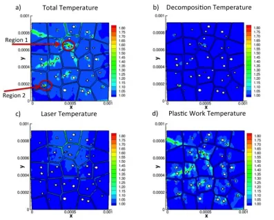
applied to the model simultaneously. ... 31 Figure 4.2: Temperature components for random void distribution and RDX

absorption coefficient α = 10 cm-1_{, normalized by the initial}

temperature of 293 K and shown at 0.632 μs. (a) Total temperature increase including effects from conduction, laser-heating,

decomposition, and plastic work heating, (b) Laser-induced

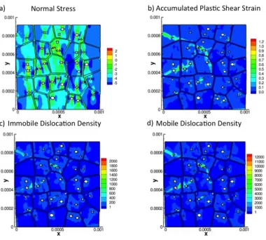
temperature increase, (c) Plastic work induced temperature increase, (d) Temperature increase due to thermal decomposition of RDX. ... 33 Figure 4.3: (a) Normal stress (normalized by static yield stress), (b) Accumulated

plastic shear strain, (c) Immobile and (d) Mobile dislocation densities from the most active slip system (010)[001] (normalized by the initial value) for random void distribution and low RDX absorption

coefficient α = 10 cm-1_{at a time of 0.632}_μ_{s. ... 35} Figure 4.4: (a) Predicted temperature, 1-D analytical solution for laser-generated

temperature (Equation (4.3)), and plastic shear strain along the vertical line taken from (b) for RDX absorption coefficient α = 10 cm-1_with random void distribution. All temperatures are normalized by the

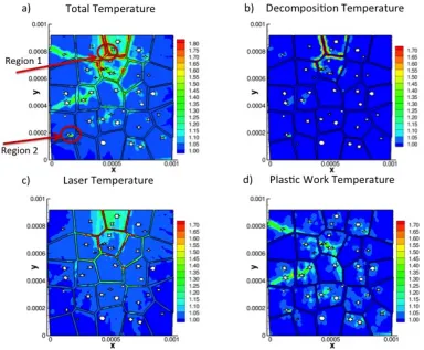
initial temperature of 293 K. ... 37 Figure 4.5: Temperature components for random void distribution and RDX

absorption coefficient α = 100 cm-1_{, normalized by the initial} temperature of 293 K and shown at a time of 0.416 μs. (a) Total temperature increase including effects from conduction, laser-heating, decomposition, and plastic work heating, (b) Laser-induced

(14)

from the most active slip system (010)[001] (normalized by the initial value) for random void distribution and RDX absorption coefficient α = 100 cm-1 at a time of 0.416 µs. ... 41 Figure 4.7: (a) Plastic shear strain distribution at time 0.416 µs for low RDX

absorption coefficient α = 10 cm-1and random voids, (b) Plastic shear strain distribution at time 0.416 µs for intermediate RDX absorption coefficient α = 100 cm-1and random voids, (c) Normalized temperature-time history for an element within the circled region, (d) Plastic shear strain-time history for an element within the circled region. The same element is used for both low and intermediate absorption cases. ... 42 Figure 4.8: Temperature components for random void distribution and RDX

absorption coefficient α = 1,000 cm-1_{, normalized by the initial} temperature of 293 K and shown at a time of 0.096 μs. (a) Total temperature increase including effects from conduction, laser-heating, decomposition, and plastic work heating, (b) Laser-induced

plastic shear strain, (c) Immobile and (d) Mobile dislocation densities from the most active slip system (010)[001] (normalized by the initial value) for random void distribution and RDX absorption coefficient α = 1,000 cm-1 at a time of 0.096 µs. ... 46 Figure 4.10: Temperature components for periodic void distribution and RDX

absorption coefficient α = 100 cm-1_{, normalized by the initial} temperature of 293 K and shown at a time of 0.488 µs. (a) Total temperature increase including effects from conduction, laser-heating, decomposition, and plastic work heating, (b) Laser-induced

plastic shear strain, (c) Immobile and (d) Mobile dislocation densities from the most active slip system (010)[001] (normalized by the initial value) for periodic void distribution and RDX absorption coefficient α = 100 cm-1 at a time of 0.488 µs. ... 48 Figure 4.12: Temperature-time history normalized by the initial temperature for

locations where a hot spot develops. ... 51 Figure 5.1: The RDX-PCTFE aggregate with boundary conditions and loading

(15)

Figure 5.2: Electric field magnitude (V/m) obtained from EM finite element solution for various energetic aggregate microstructures before

deformation. Arrows indicate the location with maximum electric field in each case. (a) Pure RDX, (b) RDX/Binder with no voids, (c)

RDX/Binder with 3 % random porosity, (d) RDX/Binder with 3 %

periodic porosity. ... 60 Figure 5.3: Maximum electric field value (MV/m) for the different energetic

microstructures. ... 62 Figure 5.4: Volumetric laser heat generation rate (W/m3) obtained from EM finite

element solution for various energetic aggregate microstructures before deformation. Arrows indicate localized areas with high laser heat generation. (a) Pure RDX, (b) RDX/Binder with no porosity, (c) RDX/Binder with 3 % random porosity, (d) RDX/Binder with 3 %

periodic porosity. ... 63 Figure 5.5: Mechanical response of RDX/binder aggregate with random void

distribution compressed to 8.4 % nominal strain with incident laser intensity of I0 = 1x105 cm-1. (a) Normal stress (normalized by static yield stress), (b) Accumulated plastic shear strain, (c) Immobile and (d) Mobile dislocation densities from the most active slip system

normalized by the initial dislocation density. ... 64 Figure 5.6: Temperature components normalized by the initial temperature of 293

K for RDX/binder aggregate with random void distribution compressed to 8.4 % nominal strain with incident laser intensity of I0 = 1x105 cm-1. (a) Total temperature increase including effects from conduction, laser heating, decomposition, and plastic work heating. Areas with

unbounded temperature increase are highlighted by arrows. (b)

Temperature increase due to thermal decomposition of RDX, (c) Laser-induced temperature increase, (d) Plastic work Laser-induced temperature increase. ... 66 Figure 5.7: Mechanical response of RDX/binder aggregate with random void

distribution compressed to 8.4 % nominal strain with incident laser intensity of I0 = 1x106 cm-1. (a) Normal stress (normalized by static yield stress), (b) Accumulated plastic shear strain, (c) Immobile and (d) Mobile dislocation densities from the most active slip system

normalized by the initial dislocation density. ... 68 Figure 5.8: Temperature components normalized by the initial temperature of 293

K for RDX/binder aggregate with random void distribution compressed to 8.4 % nominal strain with incident laser intensity of I0 = 1x106 cm-1. (a) Total temperature increase including effects from conduction, laser heating, decomposition, and plastic work heating. Areas with

(16)

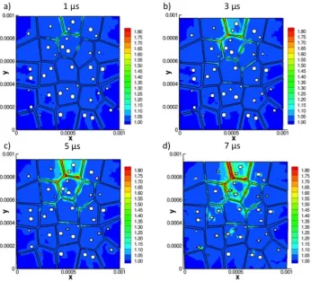
Temperature increase due to thermal decomposition of RDX, (c) Laser-induced temperature increase, (d) Plastic work Laser-induced temperature increase. ... 70 Figure 5.9: Total temperature evolution over time with laser intensity of I0 = 1x106

cm-1 at times of (a) 1 µs, (b) 3 µs, (c) 5 µs, and (d) 7 µs. All

temperatures are normalized by the initial temperature of 293 K. ... 72 Figure 5.10: Temperature-time history for locations where the first hot spot

developed. All temperatures are normalized by the initial temperature of 293 K. ... 73 Figure 6.1: The RDX-estane aggregate with boundary conditions and loading

conditions applied in the thermo-mechanical domain (left) and electromagnetic domain (right). Quantities transferred between the

domains are also shown. ... 79 Figure 6.2: Electric field magnitude (normalized by the applied electric field E0)

and laser heat generation rate for 16-grain 10% binder aggregate after 10 µs. (a) Normalized electric field, (b) Volumetric laser heat

generation rate, (c) Normalized electric field magnitude as a function of depth below the top surface at x = 0.5 mm, (d) Volumetric laser heat generation rate as a function of depth below the top surface at x = 0.5 mm. ... 81 Figure 6.3: Response of 16-grain, 10% binder aggregate after 10 µs. (a) Normal

stress (normalized by RDX yield stress), (b) Energy dissipated by viscous sliding in binder, (c) Accumulated crystalline plastic shear strain, (d) Immobile dislocation density on the most active slip system (021) [100]. ... 84 Figure 6.4: Temperature accumulation (normalized by initial temperature) in

16-grain, 10% binder aggregate after 10 µs. (a) Total temperature increase, (b) Temperature increase due to laser heating, (c)

Temperature increase due to plastic work, (d) Temperature increase due to viscous sliding. ... 85 Figure 6.5: Electric field magnitude (normalized by the applied electric field E0)

and laser heat generation rate for 49-grain, 10% binder aggregate after 10 µs. (a) Normalized electric field, (b) Volumetric laser heat

generation rate, (c) Normalized electric field magnitude as a function of depth below the top surface at x = 0.5mm, (d) Volumetric laser heat generation rate as a function of depth below the top surface at x =

(17)

strain, (d) Immobile dislocation density on the most active slip system (021) [100]. ... 89 Figure 6.7: (a) Immobile dislocation density build-up on slip system (021) [100]

after 5µs, (b) Zoomed-in view of normal stress distribution in boxed region at 5µs, (c) Normal stress–time history for circled regions, (d) Immobile dislocation density–time history on slip system (021) [100] for circled regions. All quantities are normalized by their initial values. ... 90 Figure 6.8: Temperature accumulation (normalized by initial temperature) in

Temperature increase due to plastic work, (d) Temperature increase due to viscous sliding. ... 92 Figure 6.9: Electric field magnitude (normalized by the applied electric field E0)

and laser heat generation rate for 49-grain, 30% binder aggregate after 10 µs. (a) Normalized electric field, (b) Volumetric laser heat

generation rate, (c) Normalized electric field magnitude as a function of depth below the top surface at x = 0.5mm, (d) Volumetric laser heat generation rate as a function of depth below the top surface at x =

0.5mm. ... 94 Figure 6.10: Response of 49-grain, 30% binder aggregate after 10 µs. (a) Normal

stress (normalized by RDX yield stress), (b) Energy dissipated by viscous sliding in binder, (c) Accumulated plastic shear strain, (d)

Immobile dislocation density on the most active slip system (021) [100]. . 95 Figure 6.11: Temperature accumulation (normalized by initial temperature) in

Temperature increase due to plastic work, (d) Temperature increase due to viscous sliding. ... 97 Figure 6.12: Comparison of laser-induced temperature increase vs. depth from top

surface at x = 0.5 mm in various aggregates. The full spatial laser-induced temperature distributions are shown on the right. All temperatures are normalized by the initial temperature and shown

after time of 10 µs. ... 98 Figure 6.13: Nominal stress-strain curves for various aggregates. All stresses are

normalized by the RDX yield stress. ... 100 Figure 7.1: The RDX-estane aggregate with boundary conditions and loading

(18)

Figure 7.2: Stress distribution at 8% nominal strain for quasi-static compression. (a) Lateral stress, (b) Normal stress, (c) Shear stress, (d) Hydrostatic pressure. ... 107 Figure 7.3: Stress distribution along horizontal line at y=0.6mm for (a) Aggregate

with small crystals embedded in the binder, (b) Aggregate without any small crystals. ... 109 Figure 7.4: Inelastic response at 8% nominal strain for quasi-static compression.

(a) Accumulated crystalline plastic shear strain, (b) Energy dissipated by viscous sliding in binder, (c) Gradient of accumulated plastic shear strain, ∂γ∂x, along the dashed line in (7.4a). Dashed lines indicate the location of the large grain edges. ... 110 Figure 7.5: Dislocation density activity on the most active slip system (010) [001]

normalized by the initial immobile dislocation density of 1 x 1012 m-2. (a) SSD Immobile dislocation density, (b) SSD Mobile dislocation

density, (c) Edge GND, (d) Screw GND. ... 112 Figure 7.6: (a) Spatial location of horizontal lineplots for (b-d) across binder

ligament at y = 0.6mm, (b) GND accumulation as a function of x-coordinate, (c) Normal stress as a function of x-x-coordinate, (d) Normal stress gradient in x-direction as a function of x-coordinate. Dashed

lines indicate the location of the large grain edges. ... 114 Figure 7.7: EM response of aggregate with small crystals after 2.5 µs for dynamic

compression at a strain rate of 103 s-1. (a) Electric field magnitude normalized by the applied electric field, (b) Volumetric laser heat

generation rate. ... 115 Figure 7.8: Response of aggregate with small crystals after 2.5 µs for dynamic

compression at a strain rate of 103_s-1_{. (a) Normal stress, (b) Hydrostatic} pressure, (c) Accumulated plastic shear strain, (d) viscous dissipated energy. ... 117 Figure 7.9: Response of aggregate with small crystals after 3.5 µs for dynamic

compression at a strain rate of 103 s-1. (a) Normal stress, (b) Hydrostatic pressure, (c) Accumulated plastic shear strain, (d) viscous dissipated energy. ... 118 Figure 7.10: Temperature accumulation (normalized by initial temperature of 293

K) in aggregate with small crystals after 3.5 µs for dynamic

(19)

Figure 7.11: EM response of aggregate without small crystals after 6 µs for dynamic compression at a strain rate of 103 s-1.(a) Electric field magnitude normalized by the applied electric field, (b) Volumetric laser heat

generation rate. ... 121 Figure 7.12: Response of aggregate without small crystals after 6 µs for dynamic

compression at a strain rate of 103 s-1. (a) Normal stress, (b) Hydrostatic pressure, (c) Accumulated plastic shear strain, (d) viscous dissipated energy. ... 122 Figure 7.13: Response of aggregate without small crystals after 7 µs for dynamic

compression at a strain rate of 103_s-1_{. (a) Normal stress, (b) Hydrostatic} pressure, (c) Accumulated plastic shear strain, (d) Viscous dissipated energy. ... 124 Figure 7.14: Temperature accumulation (normalized by initial temperature of 293

K) in aggregate without small crystals after 7 µs for dynamic

compression at a strain rate of 103 s-1. (a) Total temperature increase, (b) Temperature increase due to laser heating, (c) Temperature increase due to plastic work, (d) Temperature increase due to viscous sliding. ... 125 Figure 7.15: Nominal stress-strain curves for aggregates with and without small

(20)

CHAPTER 1: Introduction

1.1 Overview

Energetic materials are a class of compounds that release large amounts of stored chemical energy through an exothermic reaction at very fast reaction rates. They have many applications in components where fast energy release is required, such as rocket fuels, dynamites, and plastic bonded explosives. Detonations of these materials can result in damage and losses, so it is critical to understand and predict their response to various sources of energy, including mechanical pressures, elevated temperatures, and electromagnetic (EM) radiation.

A variety of applications involve laser irradiation of energetic materials, such as remote laser-based detection [1-5], laser machining [6], and laser-induced ignition [7]. These laser-based techniques can be performed from a standoff distance, which can help to reduce safety hazards. Extensive fracture, plastic deformation, and localized hot spot formation have been observed in energetic materials subjected to high power density laser irradiation [7,8], indicating that the interaction of EM wave propagation, heat generation, and induced high strain rate mechanical loads govern the material response. It is critical, therefore, to develop a fundamental understanding of energetic aggregates under coupled laser-thermo-mechanical loading conditions to accurately predict energetic material behavior.

(21)

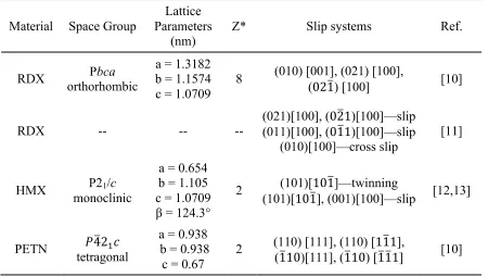
Table 1.1: Crystallographic Parameters and Slip Systems for RDX, HMX, and PETN.

Material Space Group

Lattice Parameters

(nm) Z* Slip systems Ref.

RDX _orthorhombicPbca

a = 1.3182 b = 1.1574 c = 1.0709 8

(010) [001], (021) [100],

(021) [100] [10]

RDX -- -- --

(021)[100], (021)[100]—slip (011)[100], (011)[100]—slip

(010)[100]—cross slip

[11]

HMX _monoclinicP21/c

a = 0.654 b = 1.105 c = 1.0709 β = 124.3°

2 (101)[101]—twinning

(101)[101], (001)[100]—slip [12,13]

PETN _tetragonal𝑃42!𝑐

a = 0.938 b = 0.938

c = 0.67 2

(110) [111], (110) [111],

(110)[111], (110) [111] [10] * Z denotes the number of molecules per unit cell

Due to the nature of intermolecular bonding and the size and shape of the organic molecules, slip systems available for plastic deformation are limited and unique to each material. Gallahger et. al. [10]have identified three unique slip systems in RDX through Knoop hardness indentation experiments. More recent nanoindentation experiments by Ramos et. al. [11]report observation of six total slip systems, although they also conjecture that RDX, in general, does not possess five independent slip systems to accommodate general strain distributions and there may be only three independent strain components. In HMX, the plastic deformation mechanisms are based on twinning on the (101)[101] system

(22)

slip systems are governed largely by the inter-planar spacing and shortest lattice translation distances, the complex, irregularly shaped organic molecules in energetic crystals can cause certain lattice translations on otherwise favorable slip planes to result in energetically

unfavorable inter-molecular contacts. Such steric effects appear to govern the favorable slip systems in RDX and PETN, and can explain the unique deformation mechanisms observed in these materials [10].

Energetic crystals are often embedded within a polymer binder to form energetic aggregates used as plastic bonded explosives (PBX) and solid rocket propellants [9].

Commonly used binders include estane, polychlorotriflouroethylene (PCTFE), and hydroxyl-terminated polybutadine (HTPB), which are typically present in 5 – 30% volume fractions and add mechanical stability and adhesion between the energetic crystals [14-18].

Additionally, defects including voids, solvent particle inclusions, and dislocations further contribute to the heterogeneous microstructure of energetic aggregates. The primary

initiation mechanism occurs when an external stimulus causes heat build-up in localized “hot spots” faster than it can be conducted into the bulk material [19,20]. The high temperatures generated at a hot spot accelerate the local exothermic decomposition reaction and can lead to widespread deflagration and possible detonation [21].

The heterogeneous microstructure of energetic aggregates creates multiple pathways for energy localization under EM, thermal, and mechanical stimuli. Several microstructural characteristics of energetic materials, such as voids [20,22-24], shear banding [25],

(23)

grain-boundaries (GBs), dislocations [7,29], and absorbing particle inclusions [7,30], can facilitate hot spot formation due to laser electromagnetic energy localization, which is governed by dielectric heterogeneity between the various crystal, binder, and defect constituents. Furthermore, laser energy localization can dominate at wavelengths that are weakly absorbed by the energetic crystals, due to larger penetration depths and greater interactions with defects [31,32]. EM wave scattering and attenuation within PBX materials is also strongly dependent on EM wave frequency and crystal size [33].

Modeling efforts of laser interaction with energetic materials have accounted for varying features of the material’s microstructure. Works by Abdulazeem et al. [34] and Khaneft et al. [35] used an analytical Beer-Lambert absorption profile to model laser heating of pure energetic crystals without considering any EM wave propagation effects.

(24)

an effective wave vector for THz wave propagation through granular PBX simulant aggregates.

Complex microstructure features present in energetic aggregates, such as crystal-binder interfaces, crystal morphology, polymer crystal-binder volume fraction, voids, grain

boundaries, and dislocation densities, therefore, would strongly affect EM wave propagation and the coupled thermo-mechanical behavior. Thus, an integrated modeling approach that couples the effects of high frequency EM wave propagation and thermo-mechanical behavior with the material microstructure is needed to understand and predict energetic material behavior and potential hot spot formation during laser irradiation.

1.2 General Research Objectives and Approach

The objectives of this work were to identify coupling mechanisms between the inelastic deformation, EM wave propagation, heat generation, and microstructural evolution present during laser irradiation and to develop a fundamental understanding of the coupled response of energetic aggregates. This will build knowledge of how heterogeneous

microstructural features, such as crystal sizes, interfaces and grain boundaries, dislocation densities, voids, polymer binder behavior, and electromagnetic absorption affect the response at different laser intensities and wavelengths. Such understanding will facilitate the ability to control features of energetic aggregates responsible for hot spot formation and may

ultimately lead to better methods of stand-off detection or ignition.

(25)

dislocation-coupled response of energetic aggregates under infrared laser irradiation. The model includes the effects of conduction and internal heat generation sources due to mechanical plastic deformation, the exothermic chemical decomposition reaction, and laser-induced heating, which is modeled as a function of material electromagnetic absorption coefficient and local electric field intensity.

Laser induced hot spot formation mechanisms were studied in RDX-PCTFE aggregates, where the PCTFE binder was modeled as a hypo-elastic material since laser induced temperatures were below its glass transition temperature. These aggregates were studied using both an analytical distribution for laser heating following Beer-Lambert absorption and the full EM finite element method to obtain the laser heating distribution. The laser heat distribution was then coupled to the thermo-mechanical domain to determine the effects of material absorption coefficient, laser intensity, inelastic deformation, voids, and dislocation densities on hot spot formation mechanisms.

Additionally, the coupled EM-thermo-mechanical response of RDX-estane

aggregates was studied to include the effects of viscous deformation of the binder above its glass transition temperature. Several different RDX-estane aggregates were modeled under laser irradiation and high strain rate loads to understand the effects of microstructure

morphology, aggregate size, binder volume fraction, and non-uniform crystal size distributions on EM and shear strain localization.

1.3 Dissertation Organization

(26)

(27)

CHAPTER 2: Material Constitutive Formulations and

Electromagnetic-Thermo-Mechanical Coupling

This section presents the dislocation density-based crystalline plasticity formulation used for the RDX crystals, hypo-elastic and finite viscoelastic formulations used for the polymer binder, and the governing equations for EM wave propagation in dielectric

materials. The EM-thermo-mechanical coupling mechanisms that form the basis of the laser-material interaction are presented.

2.1 Multiple Slip, Dislocation Density-Based Crystalline Plasticity Formulation The dislocation-density based crystal plasticity constitutive framework used in this study is based on the formulation developed by Zikry [38], Ashmawi and Zikry [39], and Shanthraj and Zikry [40], and is outlined in the following sections.

2.1.1 Crystalline Plasticity Kinematics

The velocity gradient tensor, , is calculated from the deformation gradient as

. (2.1)

The velocity gradient is then further decomposed into the symmetric deformation rate tensor, Dij and an anti-symmetric spin tensor Wij. It is assumed that the tensors Dij and Wij can be

additively decomposed into elastic (e) and inelastic (p) components as

, , (2.2)

where 𝑊_!"!_{includes the rigid body spin. The plastic parts are related to the crystallographic}

slip rates as

, , (2.3)

€

L_ij

€

L_ij =F ˙ _ijF_ij−1

€

D_ij =D_ije +D_ijp

€

W_ij =W_ije

+W_ijp

D_ijp

=P_ij( )α_γ_˙( )α _W ij

p

=ωij

(28)

where α is summed over all slip-systems, and and are the symmetric and

antisymmetric parts of the Schmid tensor in the current configuration, respectively. These are defined in terms of the slip plane normal (ni) and slip directions (sj) as

and . (2.4)

The effective plastic shear slip, γeff , is calculated from the plastic deformation rate tensor as

, (2.5)

to provide a measure of plastic strain accumulation over time. The objective stress rate is given by

𝜎_!"! ₌ _𝐿

!"#$ 𝐷!"−𝐷!"! −𝑊!"!𝜎!"−𝑊!"!𝜎!", (2.6)

where Lijkl is the elastic modulus fourth-order tensor of the crystal.

A power law hardening relation is assumed to obtain the slip rate (𝛾(!)_{) on each slip} system α as

no sum on α, (2.7)

where is the resolved shear stress, and is the reference shear strain-rate which

corresponds to a reference shear stress . The strain rate sensitivity parameter, m, is

obtained as

. (2.8)

€

P_ij( )α

€

ω_ij( )α

€

Pij α

( )₌1

2 si

α

( )_n

j α

( )₊_s

j α

( )_n

i α ( )

(

)

€ ωij α ( ) ₌1

2 si

α ( )_n

j α ( )₋_s

j α ( )_n

i α ( )

(

)

€

γeff =

2

3 Dij

p_D ij p_dt

∫

€ ˙ γ( )α =γ˙ ref

α ( ) τ( )α τref α % & ' ( ) * τ α ( ) τref α % & ' ' ( ) * * 1/m

( )−1

€

τ(α)

€

τ

ref

(α)

m=∂lnτ

(29)

The reference stress used is a modification of widely used classical forms [41] that relate

reference stress to immobile dislocation-density as

, (2.9)

where is the static yield stress on slip system α, G is the shear modulus, nss is the

number of slip systems, is the magnitude of the Burgers vector, and are Taylor

coefficients which are related to the strength of interactions between slip-systems [42]. Additionally, the effects of temperature are considered, where T is the temperature, T0 is the

reference temperature (293 K), and ξ is the thermal softening exponent. The Taylor

coefficients, , are obtained using Frank’s rule to determine energetically favorable

interactions for immobile dislocation density junction formation [43]. For RDX crystals, the six interactions of self-interaction, co-linear interaction, co-planar interaction, Lomer locks, glissile junctions, and Hirth locks [44] are considered, but only self-interaction is found to be energetically favorable. Thus, is assumed to be 0.6 for self-interactions on each slip

system and for the other interactions is set equal to zero.

2.1.2 Dislocation Density Evolution

Following the approach of Zikry and Kao [45], it is assumed that, for a given deformed state of the material, the total statistically stored dislocation-density, 𝜌(!)_{, can be}

additively decomposed into a mobile, 𝜌_!(!), and an immobile dislocation-density, 𝜌_!"(!) as

(2.10) € ρim €

τ

y α ( ) €

b(β)

€ a_αβ € a_αβ € a_αβ € a_αβ

ρ( )α =ρim

α

( )₊_ρ m

α

(30)

During an increment of slip, mobile dislocations may be generated, immobile dislocations may be annihilated, and junctions may be formed or destroyed due to interaction between dislocations on the various slip systems. It is assumed that the mobile and immobile dislocation-density evolution rates can be coupled through various interaction mechanisms, including the formation and destruction of junctions as the stored immobile dislocations act as obstacles for evolving mobile dislocations. Thus, the mobile and immobile dislocation density evolution rates are governed by coupled differential equations as

(2.11)

. (2.12)

The dislocation density evolution follows the formulation of Shanthraj and Zikry [43], and a brief summary is given in the following discussion. Dislocation density generation is related to Frank Read sources, where g_sour is a coefficient pertaining to an

increase in the mobile dislocation-density due to dislocation sources. Trapping of mobile dislocations due to forest intersections, cross-slip around obstacles, or dislocation interactions is described by g_mnter_{, and the immobilization of mobile dislocations is described by}g_immob.

The rearrangement and annihilation of immobile dislocations through recovery processes is given by g_recov, and is modeled using an Arrhenius relationship dependent on the frequency of

intersection between immobile and mobile dislocations, activation enthalpy, and the local temperature. These coefficients are not known beforehand, but are obtained as a function of the deformation mode as outlined in Shanthraj and Zikry [43] and shown in Table 2.1.

€

˙

ρ ( )_mα =ρ ˙ ( )_generationα −ρ ˙ _interaction( )a ₋

(31)

Table 2.1: Summary of g-Coefficients for Dislocation Density Evolution Equations

Coefficient Expression

Substituting the expressions for the coefficients in Table 2.1 into Equations (2.11-2.12), the evolution of mobile and immobile dislocation densities is obtained as

, (2.13)

. (2.14)

The dislocation activity is then coupled to the stress response through Equation (2.9).

€

gα_sour

€

bα

φ ρimβ

β

∑

€

g_mnterα ₋

€

lcf0

ρm

β

ρm

α_bα +

˙

γβ

˙

γαbβ

& ' ( ) * + β

∑

€

g_immobα ₋

€

lcf0

ρim

α ρim

β

∑

€

g_mnterα ₊

€

lcf0 ˙

γα_ρ

m α nα

βγ ρm γ _˙

γβ

bβ +

ρm β_˙ γγ bγ & ' ( ) * + β,γ

∑

€

g_immobα ₊

€

lcf0

˙

γα _ρ

im

α nα

βγ

ρimγ γ˙ β β

∑

€

gα_recov

€

l_cf₀

˙ γα ˙ γβ bβ β

∑

& ' ( ( ) * + +e

(32)

2.2 Constitutive Formulations for Polymer Binders

The constitutive relation for the polymer binder was chosen based on the polymer glass transition temperature. For the PCTFE binder, the glass transition temperature is approximately 50° C, and the temperatures due to the EM and adiabatic heating would be

lower than this glassy temperature [17]. Thus, PCTFE is modeled as a hypo-elastic material based on the first term of Equation (2.6). For the estane binder, temperatures generated by laser irradiation are well above the glass transition temperature, which is approximately -40°C [46]. Thus, a finite viscoelastic constitutive relation is used to account for the viscous relaxation behavior at operating temperatures above the glass transition of estane.

2.2.1 Finite Viscoelastic Formulation

Following a generalized Maxwell model based on the approach of Kaliske and Rothert [47], the stresses are decomposed into deviatoric and hydrostatic components, where the deviatoric component accounts for the time-history dependent viscous relaxation of the material.

The hydrostatic stress is updated using finite elasticity through the deformation-rate tensor and the Jaumann rate of Cauchy stress as

𝜎_!"#! ₌_ℂ!"#_∙_𝐷!"#₊_𝜎

!"#! ∙𝑊−𝑊∙𝜎!"#! , (2.15)

where 𝐷!"#_{is the hydrostatic component of the deformation rate tensor, 𝜎}

!"#! is the

hydrostatic stress at the current time step, and 𝑊 is the total spin tensor. ℂ!"#_{is the isotropic}

(33)

The deviatoric stress is updated as the sum of contributions from each element in the Maxwell model as

𝜎_!"#!!! ₌_𝜎

! !"#!!! + !!!!!𝐻!!!!, (2.16)

where 𝜎_!!_!"#!! _{is the deviatoric component of the lone elastic spring, and}_𝐻

!!!! is the viscous

stress corresponding to each dashpot element 𝑗. The viscous stress in each

spring-dashpot element is updated as

𝐻_!!!! =𝐻_!!∙𝑒! ∆! !_!₊ !! !! ∙ !!!! ∆! !_! ∆! !_!

∙ 𝜎_!!_!"#!! ₋_𝜎

! !"#! , (2.17)

where 𝐻_!!_{is the viscous stress at the current time step, ∆𝑡 is the time step size, 𝜏}

! is the relaxation time, 𝐺_! is the shear modulus of the spring-dashpot element, 𝐺_! is the shear

modulus of the lone spring, and 𝜎_!!_!"#_{is the deviatoric component of the lone spring at the}

current timestep. The time-temperature superposition theory of Williams, Landel and Ferry (WLF) [48] is used to modify the relaxation times through the use of the shift factor, 𝑎_!. Mas et al. [46] have fitted temperature data for estane to a WLF equation as

𝑙𝑜𝑔 𝑎_! = !!.!!!!!

!"#! !!!! , (2.18)

where 𝑇! is a reference temperature and 𝑇 is the current temperature. The relaxation time for

the Maxwell element j is related to the temperature shift factor as

(34)

2.3 Electromagnetic Formulation for Laser Wave Propagation

EM wave propagation within a material is governed by Maxwell’s equations and the material’s electrical properties. By combining Maxwell-Ampère’s and Faraday’s laws, the following differential equation is obtained to describe the electric field within the material,

where 𝐸 is the electric field vector, λ is the wavelength, ω is angular frequency, and ε0 is the

permittivity of vacuum.

∇× _!!

!∇×𝐸 − !!

!

𝜀_!−_!!!

!𝑖 𝐸 =0. (2.20)

The parameter µr is themagnetic permeability, εr is the electrical permittivity, and σ is the

electrical conductivity. The subscript r denotes that the value is relative to the corresponding property of vacuum. The electrical permittivity is also related to the material refractive index through

𝜀_! = 𝑛−𝑘𝑖 !_, _(2.21)

where the real part (n) governs wave speed and wavelength inside the material and the imaginary part (k) governs the material’s ability to absorb the EM energy.

Equation (2.20) is based on the assumption that the material has linear electrical constitutive relations and that the EM field varies harmonically with time as

𝐸 =𝐸 𝑥,𝑦,𝑧 𝑒!!"#_. _(2.22)

(35)

Most energetic materials are dielectrics with very low electrical conductivity and unique absorption spectra in the infrared wavelength range corresponding to molecular structure in the crystals [33]. Thus, it is further assumed that the material is non-magnetic (µr = 1) and non-conducting (σ = 0). With these assumptions and combining Equations (2.20

– 2.21), the EM wave propagation in a dielectric material is described by

∇× ∇×𝐸 − !!_! ! 𝑛−𝑘𝑖 !_𝐸 ₌ _0. _(2.23)

This equation is solved to obtain the electric field distribution throughout the material as a result of laser irradiation.

2.4 Coupling of Electromagnetic and Thermo-Mechanical Behavior

The primary coupling mechanism for dielectric materials occurs as the propagating EM wave is absorbed and converted to heat within the material. Assuming that all energy absorbed is converted to heat, the volumetric laser heat generation rate is equal to the EM

power loss density given by the dot product of electric field and current density (𝐽) as

𝑞!"#$% = 𝐸∙𝐽. (2.24)

Although the conduction current is assumed to be zero in such dielectric materials, bound charges switch polarization under the time-varying electric field and produce a non-zero displacement current given by

𝐽= 𝜀!(𝑛−𝑘𝑖)!!_!"!. (2.25)

(36)

𝑞_!"#$% = 𝐸 !! !𝑐𝜀!𝑛

!!"

! . (2.26)

Equation (2.26) can also be written as the product of the electric field intensity, I, and material absorption coefficient, α, by considering their relationship with electric field and material refractive index as

𝛼= !!"_! , (2.27)

𝐼= 𝐸 !!_!𝑐𝜀_!𝑛. (2.28)

In addition to the laser-induced heating, thermo-mechanical heat generation sources are assumed to occur. During high strain-rate deformation, heat is generated in crystalline materials as the material undergoes plastic work and builds up much faster than conduction away from the deformed area can occur. Thus, adiabatic heat generation due to mechanical energy in crystalline materials is given as

𝑞mechanical=χ σij’ DijP, (2.29)

where χ is the fraction of plastic work converted to heat, and 𝜎_!"!_{is the deviatoric stress.}

Energetic crystals can also produce heat through an exothermic thermal decomposition reaction, which is assumed to occur as a single-step Arrhenius exothermic process [49] as

𝑞decomposition=ρΔHZe -Ea

RT, (2.30)

where ρ is the mass density, ΔH is the heat of decomposition, Z is a pre-exponential factor, 𝐸_! is the activation energy of decomposition, R is the universal gas constant, and T is the

(37)

𝑞_!"#$%&# = !!!!! ∶ !!!!!

! !! !! !!

!!! . (2.31)

Equations (2.26, 2.29 – 2.31) are used as heat sources to the Fourier heat equation, which couples their effects with conduction and temperature build up. Thus, the temperature distribution (T) resulting from dielectric laser heating, adiabatic heat generation from plastic work, viscous dissipative heating, and thermal decomposition mechanisms is obtained as

ρc_p ∂T

∂t =λ∇

2_T+𝑞

mechanical+𝑞decomposition+𝑞laser+𝑞viscous, (2.32)

(38)

CHAPTER 3: Numerical Methods

The computational framework used to couple the high frequency electromagnetic wave propagation discussed in Section 2.3 with the evolution of stresses, temperatures, and other thermo-mechanical quantities is presented in Section 3.1. Additionally, the specialized finite element scheme used in the thermo-mechanical domain to obtain the velocity gradient tensors and temperature distribution is outlined in Section 3.2.

3.1 Framework for Coupling EM and Thermo-Mechanical Domains

EM wave propagation, thermal conduction, and inelastic deformation occur on different time and length scales associated with the physical system of interest. For thermo-mechanical processes, the length scale is related to the microstructural features and

temperature gradients that must be resolved, and the time scale is associated with the propagating inelastic wave speed and material thermal diffusivity. The various

microstructural constituents of energetic aggregates range between 10 to 200 µm, and the timescale associated with dynamic inelastic wave propagation ranges from ms to ns. The time and length scales of interest for EM wave propagation are associated with the EM wavelength and wave speed in a medium, and finite elements used to discretize Equation (2.23) are approximately on the order of five times smaller than the EM wavelength. This requires elements no larger than 2 µm to resolve the infrared wavelengths considered in this study, which is significantly smaller than element sizes required to resolve the

(39)

wave speed, and EM waves will traverse a given distance several orders of magnitude faster than inelastic waves.

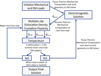
A different finite-element mesh and solution must, therefore, be used for the EM domain, than the one used for the thermo-mechanical domain. This is accomplished through a computational framework that solves the EM and thermo-mechanical problems using separate domains and passes information sequentially between them (Figure 3.1).

Figure 3.1: Computational algorithm for coupled electromagnetic-thermo-mechanical model.

(40)

inelastic wave speed, it is assumed that the electric field has reached steady state conditions during a single thermo-mechanical time step. The commercial software COMSOL

Multiphysics is used to obtain the electric field distribution according to the finite element solution of Equation (2.23), and the associated volumetric laser heat generation rate is mapped to the thermo-mechanical domain.

As shown in Figure 3.1, an initial EM solution is obtained before the thermo-mechanical computation is initiated. The laser heat distribution 𝑞_!"#$% is passed to the

thermo-mechanical domain and mapped onto the thermo-mechanical mesh. The multiple-slip dislocation density based crystalline plasticity constitutive model is then used to obtain thermo-mechanical deformation and heat generation, which are then combined with the laser heat generation to obtain the temperatures by Equation (2.32).

Since changes in the microstructure may affect EM wave propagation, it is necessary to consider this effect by re-calculating the laser heat generation rate using the current deformed microstructure. However, to do this at every time step would be computationally expensive and is not necessary as long as the deformation that occurs during a single time step is relatively small. Therefore, information is passed between the different domains at nominal strain increments of 2.5%. If the nominal strain is less than 2.5% since the last EM update, the thermo-mechanical computation continues on to the next time step and uses the laser heating values obtained from the most recent EM update. If the nominal strain

(41)

𝑞!"#$% is then mapped back to the thermo-mechanical domain and used until the next EM update.

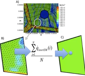
3.1.1 Mapping Methods Between EM and Thermo-Mechanical Domains

For the energetic aggregates and laser wavelengths considered in this study, the elements used in the EM domain are 10-20 times smaller than the elements used in the thermo-mechanical domain. Consequently, the mapping method shown in Figure 3.2 is used to map the laser heat generation rate from the EM domain to the thermo-mechanical domain.

(42)

The thermo-mechanical mesh is superimposed on the EM mesh (Figure 3.2(a)), and the EM elements are sorted according to which thermo-mechanical element they are located within. The laser heat generation rate assigned to each thermo-mechanical element

(𝑞_!"#$%&') is then determined by averaging the laser heat generation rate of all the EM

elements (𝑞_!"#$%&') contained inside that particular thermo-mechanical element (Figure 3.2(b-c)) as

𝑞_!"#$%&' = !!!!!!"#!"#$(!)

! , (3.1)

where N is the number of EM elements contained inside each thermo-mechanical element. When updating the EM solution, the current nodal coordinates of the

thermo-mechanical mesh are used to create a new model in the EM domain with geometry identical to the deformed thermo-mechanical domain. A new EM mesh is then generated for this configuration, and it is used to obtain the updated electric field distribution and laser heat generation rate from Equations (2.23) and (2.26).

3.2 Numerical Methods in the Thermo-Mechanical Domain

The total deformation rate tensor, 𝐷!", and the plastic deformation rate tensor, 𝐷!"!, are

(43)

3.2.1 Determination of the Total Velocity Gradient

The total velocity gradient is calculated from the nodal displacements obtained by finite element analysis with Q4 quadrilateral elements. The deformation calculated by the finite element method is used to calculate the total velocity gradient in accordance with Equation (2.1). For static analysis, an incremental, iterative approach using the quasi-Newton BFGS scheme is used to determine the nodal displacements. For dynamic analyses, an implicit Newmark- , iterative approach using BFGS to solve the finite element equations

linearized about at each timestep is used. Trapezoidal values of and were

chosen for unconditional stability of the finite element method. Details for this dynamic approach are given by Shanthraj and Zikry [43].

To avoid numerical locking due to incompressible pressure constraints, 1-point integration of the Q4 quadrilateral element is used, which has the added benefit of reduced computational time. However, reduced integration can lead to the zero-energy numerical instability of hourglassing. Stiffness-based hourglass control is implemented to control the hourglass instability following the method of Flanagan and Belytschko [51].

3.2.2 Determination of the Plastic Velocity Gradient

The objective stress rate is coupled with the time derivative of the resolved shear stresses to determine the resolved shear stresses on each slip plane given by

, (3.2)

, (3.3)

€

β

€

tn

€

β=1 4

€

γ=1 2

€

˙

τ( )α = d dt Pij

α ( )_σ

ij

(

)

˙

τ ( )α =C_ijklP_ij( )α_D

(44)

Equation (3.3) can be expanded to

, (3.4)

where the reference stress is a function of the immobile dislocation density. The slip rates can be determined using the resolved shear stress (Equation (2.9)). The plastic deformation rate tensor and spin rate tensor can then be used along with the Schmid tensor and slip rates to determine the plastic velocity gradient (Equation (2.3)).

The elastic spin rate tensor can be determined as a function of the total spin rate tensor and the plastic spin rate tensor using Equation (2.2). It was assumed in the derivation of Equation (3.4) that the time rate of change of the slip normals and directions is related to the lattice spin as

and . (3.5)

The non-linear ODE’s governing the resolved shear stresses and dislocation density evolution necessitate a solution method that is both accurate and stable due to their non-linear nature and the possibility of numerical stiffness [38]. The non-linear nature of the problem requires a solution method with high order accuracy, while the possibility of numerical stiffness requires a solution method that is stable and will not propagate error due to stiff behavior.

An adaptive timestep fifth-order accurate step halving Runge-Kutta method is

employed. Two approximate solutions are taken using the fourth-order Runge-Kutta method,

€

˙

τ ( )α =2µP_ij( )α _D

ij− Pij

ξ ( )_γ_˙ ref ξ ( ) τ( )ξ τref ξ ( ) ' ( ) ) * + , , 1 m

ξ=1,nss

∑

. / 0 0 0 1 2 3 3 3 € ˙

n _i( )α =W_ijeln_j

€

˙

(45)

(3.6)

(3.7)

The two solutions are combined to yield

, (3.8)

where is the local truncation error, which is used to measure the accuracy of the

solution. If the accuracy is not less than a specified tolerance, , the timestep size is

reduced by

, (3.9)

where is the new timestep size, is the initial timestep size, and is used to keep

the new timestep small enough to be accepted.

When the timestep is becomes excessively small, the timestep restriction can be due to stability issues caused by numerical stiffness [38]. The integration method is then switched to the first-order accurate, unconditionally stable, backward Euler method,

, (3.10)

which is solved using quasi-Newton iteration.

3.2.3 Finite Element Representation of Thermal Conduction

Temperatures are obtained from the discretized finite element heat conduction equation,

C 𝑇 + K 𝑇 = 𝑅! , (3.11) €

τ

₍

t+h

₎

=τˆ 1+

( )

h 5

φ+O h

( )

6 +⋅ ⋅ ⋅

€

τ

(

t+2

₍

h/2

₎

)

=τˆ 2+2

(

h/2

)

5

φ+O h

( )

6 +⋅ ⋅ ⋅

€

τ

₍

t+h

₎

=τˆ 2+Δ1 15+O h

6

( )

€

Δ1=τ ˆ 1−τ ˆ 2

€

Δ0

€

h_new=Fh_old Δ0

Δ1 0.20 € hnew € hold € F €

τn+1 α ( ) ₌_τ

n

α

( )₊_hf _τ

n+1 α ( )_,_t

n+1

(46)

where 𝐶 is the matrix of coefficients proportional to temperature rate of change, 𝑇 is the

vector of change in nodal temperatures, 𝐾 is a matrix of coefficients proportional to temperature, 𝑇 is the vector of nodal temperatures, and 𝑅_! is the vector of nodal input heat sources for mechanical, decomposition, and laser energies. The elemental matrices of these quantities are given by

𝐶!"! = 𝑁! 𝑁 𝜌 𝑐!𝑑𝑉, (3.12)

𝐾_!"! = 𝐵! _𝜅 _𝐵 _{𝑑𝑉, (3.13)}

𝑅!"! = 𝑁! 𝑄𝑑𝑉, (3.14)

where 𝑁 is the vector of shape functions, 𝐵 is the strain-displacement matrix, and 𝜅 is the matrix of thermal conductivities. The elemental heat generation rate, Q, is the sum of heat generation sources within the element obtained from Equations (2.26) and (2.29 – 2.31).

The time-varying temperature histories are obtained by direct time integration of Equation (2.32) as follows

!

!" 𝐶 +𝛽[𝐾] 𝑇 !!! = !

(47)

CHAPTER 4: Laser Interaction Effects of EM Absorption and

Microstructural Defects on Hot-Spot Formation in RDX-PCTFE Energetic

Aggregates

4.1 Introduction

It is necessary to understand the effects of microstructure on the response of energetic aggregates to incident laser energy, thermal, and mechanical loads, and to identify the

mechanisms that contribute to hot spot formation and possible detonations. The complex microstructure of these materials, in conjunction with their mechanical, chemical, and electrical properties, greatly affects their sensitivity to detonation due to the interrelated effects of high mechanical pressures, temperatures, and electromagnetic energy.

Hence, the main objective of this study is to investigate and understand the coupled effects of microstructural crystal-binder interactions, dislocation-density evolution, void distributions and material electromagnetic absorption properties on the thermo-mechanical response and hot spot formation mechanisms in energetic aggregates subjected to

simultaneous laser energy and dynamic pressure loads. The effects of electromagnetic absorption coefficient coupled with void distribution and spacing, grain morphology, crystal-binder interactions, and dislocation densities were analyzed to determine their influence on the time, location, and mechanisms of hot spot formation.

4.2 Results