Numerical Study of Two Problems in Fluid Flow: Cavitation and Cerebral Circulation

(1)

DeVAULT, KRISTEN J. Numerical Study of Two Problems in Fluid Flow:

Cavitation and Cerebral Circulation. (Under the direction of Dr. Pierre A. Gremaud).

Two different computational models of fluid flow are considered. First, the pos-sibility of cavitation is investigated numerically in two and three dimensions for the spherically symmetric, barotropic, Navier-Stokes equations. A splitting method is derived in order to allow the use of known solutions to the corresponding inviscid Euler equations. Results indicate cavitation is possible in the presence of high Mach numbers. This work is intended to be a stepping off point in the search for analytic solutions showing cavitation in multi-dimensional compressible flows.

(2)

by

Kristen Jean DeVault

A dissertation submitted to the Graduate Faculty of North Carolina State University

in partial fullfillment of the requirements for the Degree of

Doctor of Philosophy

Applied Mathematics Raleigh, North Carolina

February 18th, 2008

APPROVED BY:

Dr. Pierre A. Gremaud Dr. Alina Chertock Chair of Advisory Committee

Dr. C. Tim Kelley Dr. Mette S. Olufsen

(3)

DEDICATION

(4)

BIOGRAPHY

Kristen Jean DeVault was born in Ludington, Michigan and grew up in Laurel, Mary-land. She graduated from the University of Maryland with a Bachelor of Science degree in Mathematics in May of 2002. After graduating, she went on to work as a Mathematician for the Department of Defense at the Naval Surface Warfare Cen-ter in Dahlgren, Virginia. While there, she began taking graduate courses part-time through the University of Virginia.

(5)

ACKNOWLEDGMENTS

First and foremost, I would like to thank my advisor, Pierre Gremaud, for his con-tinued help and support through this process. He has always provided encouragement and guidance when needed.

I would like to recognize and thank Kris Jenssen for his assistance on the cavitation portion of this work, and Mette Olufsen for her assistance on the blood flow portion, and for serving on my committee. I would also like to thank Alina Chertock, Tim Kelley, Ralph Smith, and S. Pal Arya for serving on my committee.

I would like to thank Vera Novak and Peng Zhao for collecting and providing the data needed to complete much of this work, and Guillaume Vernieres for his help with the parameter fitting portion of the blood flow project.

(6)

LIST OF TABLES

Table 2.1 Coefficients associated with BDF methods for k= 1,2,3,4. . . 19

Table 4.1 Parameters in single vessel model after nondimensionalization. . . 63 Table 4.2 Relative error statistics for the spatial and temporal resolution tests. . . 77 Table 4.3 Specific geometry of the Circle of Willis used for the calibration and

validation of the model. The values in italics were missing from the data and had to be estimated. . . 80 Table 4.4 Results of a simple sensitivity analysis. As expected, the solution in

a given outflow vessel is highly sensitive to its own resistance parameters, moderately sensitive to the resistance parameters of the other outflow vessels, and insensitive to the compliances. . . 85 Table 4.5 Complete CoW - Symmetric Geometry: After the stochastic version of

the model has been run to create 20 realizations, the mean velocity profile is calculated in each vessel. These curves are then compared to the means calculated from the data. The table above shows the percentage of time the model mean is within one or two standard deviations (σ) of the data mean (µ) in each of the six outflow vessels.. . . 90 Table 4.6 Updated geometry data for asymmetric CoW. . . 90 Table 4.7 Complete CoW - Asymmetric Geometry: The table above shows the

percentage of time the model mean is within one or two standard deviations (σ) of the data mean (µ) in each of the six outflow vessels. . . 91 Table 4.8 List of common anatomical variations within the Circle of Willis and the

(10)

LIST OF FIGURES

Figure 2.1 Chebyshev polynomials of degree n = 0,1,2,3,4,5. . . 6 Figure 2.2 Accuracy of Chebyshev differentiation versus finite difference

differen-tiation as a function of the number of nodes. (top) The error in the Chebyshev method decreases much faster than that of the finite difference method until it reaches machine precision. (bottom) The finite difference scheme shows 2nd order convergence while the Chebyshev method shows spectral convergence. 14 Figure 2.3 Comparison of the maximum error over space and time versus the

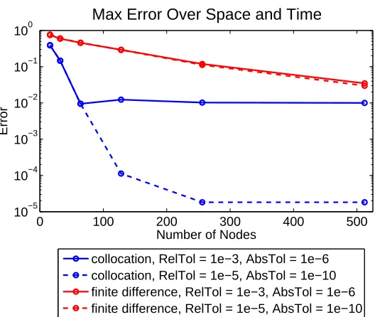
number of nodes for the solution of the advection initial-boundary value prob-lem (2.13) using MATLAB’s ode15s _{solver in time with Chebyshev}

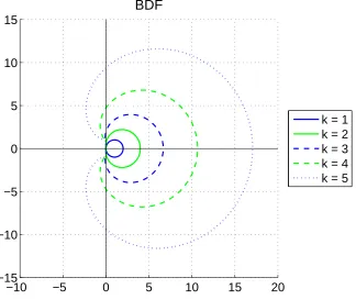
colloca-tion or finite difference derivatives in space. The solucolloca-tion using the Chebyshev collocation derivative achieves a smaller amount of error with 64 nodes than the centered finite difference method achieves with 512 nodes. The tolerances given are the relative and absolute tolerance parameters for the MATLAB solver. The fact that the two finite difference curves are almost identical in-dicates that the total error is dominated by the error in the finite difference approximation of the spatial derivative. The collocation curves, on the other hand, are quite different. This indicates that the overall error is dominated by the error from the timestepping scheme. . . 16 Figure 2.4 Stability regions for BDF methods with k = 1,2,3,4,5. In each case,

the stability region is the area outside the curve. . . 23

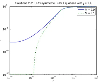
Figure 3.1 Solutions to the axisymmetric Euler Equations in 2 spatial dimensions with γ = 1.4. Note the difference in behavior of the density as r approaches 0. Cavitation occurs for M = 3.1 (dashed line), but not for M = 2.9 (solid line). This is in agreement with the critical Mach number shown in Figure 3.2(b). . . 43 Figure 3.2 Numerically calculated integral curves and critical Mach numbers

(11)

Figure 3.4 Phase diagrams for the Euler and Navier-Stokes solutions at the node closest to the origin in 3-D with _M = 1.2 (no vacuum) and _M= 2.7 (vac-uum). For the Navier-Stokes solution, the Reynolds number is _Re= 106_{.. . . 49}

Figure 3.5 One-dimensional Navier-Stokes and Euler solutions forγ = 1.4, _M= 10. Left: solutions at time t = 0.5 with _Re = 104_{; Right: solutions at}

time t = 0.002 with Re = 106_{. For these values, both the one-dimensional}

Euler solution and the multi-dimensional Navier-Stokes solution show vacuum formation, while the 1-D Navier-Stokes solution does not. . . 50 Figure 3.6 Vacuum formation regions for 2- and 3-D barotropic flows with γ =

1.4. Left: 2-D; Right: 3-D. . . 51

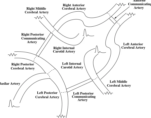
Figure 4.1 Diagram of the Circle of Willis (CoW). . . 53 Figure 4.2 Comparison of calculated velocities in the LMCA using different values

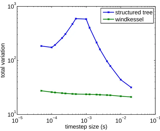
ofτ andγ. Based on this preliminary test, there does not seem to be evidence that the alternate values give a better fit to the data. . . 64 Figure 4.3 Comparison of total variation in solution for windkessel outflow versus

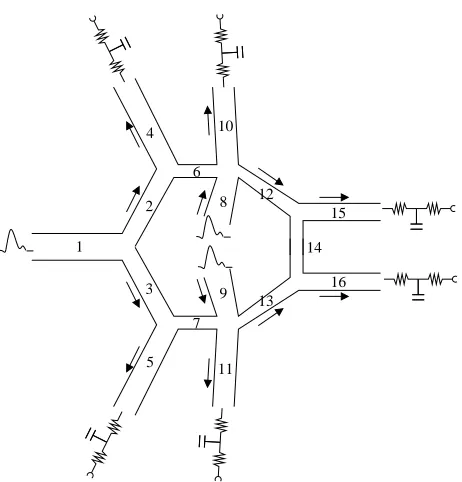
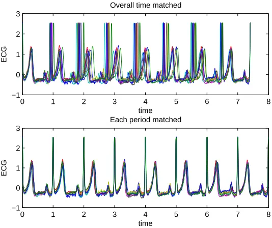
structured tree outflow in a single vessel. The total variation increases rapidly in the structured tree case due to the added high frequency components which are not fully resolved. Once all high frequency components have been resolved, the total variation drops. This limitation on the timestep makes the structured tree boundary condition less than ideal for our purposes. . . 74 Figure 4.4 Example of data collected in the right internal carotid artery (RICA). 78 Figure 4.5 Mock-up of the Circle of Willis which corresponds to Table 4.3 . . . 79 Figure 4.6 The data must be post-processed in order to ensure consistency across

data sets. Two possible options are shown above. (top) The overall length of eight periods is even. (bottom) The length of each period is stretched to one second. Clearly, the second option makes the ECG output more consistent. 81 Figure 4.7 Comparison of model velocity results to velocity data in the RMCA

(12)

blood pressure data in the finger using the original and EnKF parameters. (b) Comparison of model velocities (top) and model blood pressures (bottom) to data after scaling the EnKF resistance parameters by .7. . . 84 Figure 4.9 Sensitivity curves versus ranking of the windkessel boundary condition

parameters. The curves show a clear cutoff after the first two parameters and again after the next ten parameters. These correspond to the sections marked in Table 4.4. . . 86 Figure 4.10 Mean inflow velocities with associated standard deviation bars from

data. . . 87 Figure 4.11 Mean outflow velocities with associated standard deviation bars from

data. . . 88 Figure 4.12 Comparison of left and right mean outflows. . . 90 Figure 4.13 Comparison of model results to data in the LMCA over multiple

car-diac cycles. . . 91 Figure 4.14 Mean outflow velocities resulting from running the stochastic version

of the model over 20 realizations. . . 92 Figure 4.15 Comparison of perfusions for different geometries in the absence of a

stroke. . . 95 Figure 4.16 Comparison of perfusions for different geometries in the absence of a

stroke. (Alternative Representation) . . . 96 Figure 4.17 Inflow velocity over time in the event of a stroke. . . 96 Figure 4.18 Even though the change in inflow is abrupt in the event of a stroke,

the blood flow velocity returns to a periodic state very quickly. . . 97 Figure 4.19 Comparison of perfusions in subject with complete CoW after different

types of strokes. . . 98 Figure 4.20 Comparison of perfusions in subject with complete CoW after different

types of strokes. (Alternative Representation) . . . 98 Figure 4.21 Comparison of perfusions in subject with an extra ACoA after different

(13)

Figure 4.22 Comparison of perfusions in subject with extra ACoA after different types of strokes. (Alternative Representation) . . . 99 Figure 4.23 Comparison of perfusions in subject with missing LACA, segment 1

after different types of strokes. . . 100 Figure 4.24 Comparison of perfusions in subject with missing LACA, segment 1

after different types of strokes. (Alternative Representation) . . . 101 Figure 4.25 Comparison of perfusions in subject with missing ACoA after different

types of strokes. . . 101 Figure 4.26 Comparison of perfusions in subject with missing ACoA after different

types of strokes. (Alternative Representation) . . . 102 Figure 4.27 Comparison of perfusions in subject with missing LPCoA after

differ-ent types of strokes. . . 103 Figure 4.28 Comparison of perfusions in subject with missing LPCoA after

differ-ent types of strokes. (Alternative Represdiffer-entation) . . . 104 Figure 4.29 Comparison of perfusions in subject with missing L&R PCoAs after

different types of strokes. . . 104 Figure 4.30 Comparison of perfusions in subject missing both PCoAs after

differ-ent types of strokes. (Alternative Represdiffer-entation) . . . 105 Figure 4.31 Comparison of perfusions in subject missing all communicating

arter-ies after different types of strokes.. . . 105 Figure 4.32 Comparison of perfusions in subject missing all CoAs after different

types of strokes. (Alternative Representation) . . . 106 Figure 4.33 Comparison of perfusions in subject with missing LPCA, segment 1

after different types of strokes. . . 107 Figure 4.34 Comparison of perfusions in subject with missing LPCA, segment 1

(14)

Chapter 1 Introduction

Computational models have vastly varied uses in the field of applied mathematics. On the more theoretical side, they can be used as a tool to gain insight into as yet unsolved theoretical problems giving other researchers a better idea of what to be looking for. In a more applied and interdisciplinary direction, they can be used to investigate biological variations within the human body. Not to mention the myriad of applications in between. In this work, two different computational models relating to fluid flow will be considered: cavitation in compressible flows and cerebral circulation in the Circle of Willis.

(15)

to get accurate results in a reasonable amount of time.

There are also a number of differences between the two problems. In the cavitation problem, pockets of zero density within the solution are sought. Thus, the density must be allowed to change during the simulation requiring us to consider the equations for compressible fluid flow. For the cerebral blood flow problem, blood, which is essentially incompressible, is being modeled, so the incompressible fluid flow equations are used. Since there are known solutions to the inviscid equations corresponding to the viscous cavitation model, a splitting method (see section 3.8.3) will be used to allow the known inviscid solutions to be taken into account when solving the viscous equations. For the blood flow problem, there are no related solutions and therefore a simpler unsplit method is used. The final major difference in the two problems is the size of the Reynolds numbers considered. The Reynolds number is inversely proportional to the viscosity (see section 4.15). In the cavitation problem, fluid with low viscosity and therefore high Reynolds numbers will be considered. Conversely, in the cerebral circulation problem the flow of blood, which has a much lower Reynolds number, will be considered.

(16)

Chapter 2 Numerical Considerations

In the applications considered in the following chapters, accuracy and speed will be important factors in choosing the numerical methods used to solve the given problems. One easy way to speed up a method is to reduce the number of nodes at which a solution is calculated. However, reducing the number of nodes often leads to decreases in the accuracy of the method. Thus, it is important to look for methods that achieve high levels of accuracy with a small number of nodes. One such class of methods are collocation methods.

2.1 Spatial Discretization

(17)

2.1.1 Lagrange Interpolation

One example of interpolation using algebraic polynomials is Lagrange interpola-tion. Given a set of n+ 1 points in R_{, with}

x0 < x1 <· · ·< xn, consider the Lagrange Polynomials

Li(x) = n

Y

k=0, k6=i

x₋xk

xi−xk

, (2.1)

for i= 0,1, . . . , n, which have the properties

Li(x) _{∈ P}n, i= 0,1, . . . , n,

Li(xj) = δij =

(

1 i=j

0 i₆=j ,

where Pn is the set of polynomials of degree less than or equal to n.

Theorem 2.1 (Lagrange Interpolation) Given n + 1 data points (xi, fi), i = 0,1, . . . , n with xi 6= xj for i 6= j, the unique polynomial p(x) ∈ Pn which

inter-polates the data points is

p(x) = n

X

i=0

fiLi(x) = n

X

i=0 fi

n

Y

k=0, k6=i

x₋xk

xi−xk

. (2.2)

Proof. Suppose there exists ˜_Li such that ˜Li ∈ Pn and ˜Li(xj) =δij.

Then Li−L˜i ∈ Pn and Li −L˜i has n + 1 distinct zeros, namely x0, x1, . . . , xn.

Thus, _Li−L˜i = 0, or Li ≡L˜i. Therefore the Li’s are unique making p(x) unique as well.

Finally, p(xj) = Pn

(18)

Theorem 2.2 Let x0, x1, . . . , xn be n + 1 distinct points in [a, b]. Then if f ∈

Cn+1_([_{a, b}_])_{, for each} _x_∈_[_{a, b}_]_{, there exists a} _ξ₍_x₎ _in ₍_{a, b}₎ _{such that}

f(x)−p(x) = f

(n+1)₍_ξ₍_x₎₎

(n+ 1)! n

Y

i=0

(x−xi) (2.3)

where p(x) is the Lagrange interpolating polynomial defined above. Proof. Forx=xk,f(xk) =p(xk) and f(n₍+1)_n_+1)!(ξ(x))Qn

i=0(x−xi) = 0.

Forx fixed with x6=xk, k= 0,1, . . . , n, define g(t) fort ∈[a, b] as follows

g(t) =f(t)₋p(t)₋(f(x)₋p(x)) n

Y

i=0

t₋xi

x₋xi

.

Then, if t = xk, g(xk) = f(xk)₋p(xk)₋(f(x)₋p(x))Qn

i=0

xk−xi

x−xi = 0. Similarly,

if t = x, g(x) = f(x)₋p(x)₋(f(x)₋p(x))_· 1 = 0. Therefore, g _{∈ C}n+1_([_{a, b}_])

and vanishes atn+ 2 points. Thus, by the generalized Rolle’s Theorem, there exists

ξ_∈(a, b) such thatg(n+1)₍_ξ_{) = 0. Which means}

0 =g(n+1)(ξ) = f(n+1)(ξ)−p(n+1)(ξ)−(f(x)−p(x)) d n+1 dtn+1

n

Y

i=0 t−xi

x₋xi

! ξ .

Since p ∈ Pn, p(n+1) = 0. Also, Qn

i=0 xt−−xxii is a polynomial of degree n + 1 in t, or

more precisely

n

Y

i=0 t−xi

x₋xi

= t

n+1

Qn

i=0(x−xi)

+q(t),

where q(x)∈ Pn. Thus,

dn+1 dtn+1

n

Y

i=0 t−xi

x₋xi

!

= Qn(n+ 1)!

i=0(x−xi)

.

Substituting this into the relation above, gives

0 =f(n+1)(ξ)−(f(x)−p(x))Qn(n+ 1)!

i=0(x−xi) ,

or,

f(x)−p(x) = f

(n+1)₍_ξ₎

(n+ 1)! n

Y

i=0

(19)

−1 −0.5 0 0.5 1 −1

−0.5 0 0.5 1

Chebyshev Polynomials of Degree n=0,1,2,...,5

n = 0 n = 1 n = 2 n = 3 n = 4 n = 5

Figure 2.1: Chebyshev polynomials of degree n= 0,1,2,3,4,5.

Using Lagrange interpolation on equally spaced nodes can still lead to large amounts of error. However, if well chosen unevenly spaced nodes are used, the error can be reduced significantly. The next section will discuss a family of polynomials known as Chebyshev polynomials and show how they are related to choosing the best set of unevenly spaced nodes to get the smallest error between the function and its interpolant.

2.1.2 Chebyshev Polynomials

The Chebyshev polynomials are defined recursively as follows

T0(x) = 1, T1(x) = x,

Tn(x) = 2xTn−1(x)−Tn−2(x), n≥2.

(20)

Proposition 2.1 The Chebyshev polynomials Tn(x), defined recursively above, are equivalent to cos(narccosx) on [−1,1].

Proof.

• n= 0 : T0(x) = 1 = cos(0·arccosx) • n= 1 : T1(x) =x= cos(1·arccosx)

• n > 1 : assume Tk(x) = cos(karccosx) for k = 0,1, . . . , n−1 and let y = arccosx. Then

Tn(x) = Tn(cosy)

= 2 cos(y)Tn−1(cos(y))−Tn−2(cos(y))

= 2 cos(y) cos ((n₋1)y)₋cos ((n₋2)y) = 2

1

2(cos(ny) + cos ((n−2)y))

−cos ((n−2)y) = cos(ny) + cos ((n₋2)y)₋cos ((n₋2)y)

= cos(ny)

= cos(narccosx).

⇒ By induction, Tn(x) = cos(narccosx) for anyn ≥0.

In order to derive the optimal nodes to be used in the interpolation, the following result will be needed.

Proposition 2.2 (Optimality Property of Chebyshev Polynomials) Let_P˜nbe

the set of polynomials of degree n with leading coefficient 1. Then

max

−1≤x≤1

|Tn(x)|

2n−1 ≤₋max₁_≤_x_≤₁|p(x)|

for any p∈P˜n.

Proof. Assume there exists p(x)∈P˜n such that max

−1≤x≤1|p(x)|<

(21)

and let

r(x) = Tn(x)

2n−1 −p(x).

Since Tn(x)

2n−1 is in ˜Pn and p(x) is in ˜Pn,r(x) is of degree less than or equal ton−1. Consider x′

k = cos kπn

, for k= 0,1, . . . , n.

Tn(x) = cos (narccosx)

⇒ T_n′(x) = nsin (√narccos(x))

1−x2

⇒ T′

n(x′k) = Tn′

cos kπ n

= nsin narccos cos kπ

n

q

1₋cos2 kπ n

= nsin (kπ)

sin kπ_n = 0 for k= 0,1, . . . , n.

Thus the x′

ks are extreme points of Tn(x) and

Tn(x′

k) = Tn

cos kπ n = cos narccos cos kπ n

= cos(kπ) = (−1)k

⇒ r(x′

k) =

Tn(x′

k) 2n−1 −p(x

′

k) = (₋1)k

2n−1 −p(x

′

k). Also, by assumption, max−1≤x≤1|p(x)| ≤ ₂n1−1, so

k even: r(x′

k) = 1

2n−1 −p(x

′

k)

> 1

2n−1 −

1 2n−1 = 0 k odd: r(x′_k) = −1

2n−1 −p(x

′

k)

< −1

2n−1 +

1

2n−1 = 0.

Therefore, r(x) changes sign at least n times on [−1,1]. But r(x) is of degree less than or equal to n₋1, so r(x)_≡0 makingp(x) = Tn(x)

2n−1. Thus, max

−1≤x≤1|p(x)|=

1

(22)

⇒ max

−1≤x≤1|p(x)| ≥

1

2n−1 = max₋₁_≤_x_≤₁

Tn(x) 2n−1

.

2.1.3 Optimal Node Placement

From the error formula (2.3), it is apparent that to reduce the error in the ap-proximation, one must work with the location of the nodes since one has no control over ξ(x). Therefore, a polynomial of degree n+ 1 with leading coefficient 1, which has the smallest maximum value is desired. By the optimality property just shown (Proposition 2.2), it is known that this polynomial is the (normalized) Chebyshev polynomial of degreen+ 1. Since the desired Chebyshev polynomial is defined on the interval [₋1,1], in order to use an arbitrary interval [a, b], a change of variables that maps -1 to a and 1 to b must be used, i.e.

˜

x= 1

2[(b−a)x+a+b].

Since the nodes used in the Lagrange interpolation are the roots of the polynomial in the error formula, the nodes are chosen to be the zeros of Tn+1, namely

xk = cos

(2k+ 1)π

2(n+ 1)

,

for k = 0,1,2, . . . , n.

Notice that the nodes above do not contain the endpoints of the domain. Some-times is it necessary to include one or both of the endpoints as nodes. The so-called Gauss-Radau nodes (containing one endpoint) and Chebyshev-Gauss-Lobatto nodes (containing both endpoints) can be derived in a similar manner. In summary, the best choice of nodes on the interval [−1,1] is one of the following, depending on whether or not nodes at the endpoints are desired:

• Chebyshev-Gauss

xk = cos

(2k+ 1)π

2(n+ 1)

(23)

• Chebyshev-Gauss-Radau

xk = cos

2πk

2n−1

, for k = 0,1, . . . , n₋1, (2.5)

• Chebyshev-Gauss-Lobatto

xk = cos

kπ n

, for k = 0,1, . . . , n. (2.6)

2.2 Collocation Methods

Collocation methods are designed to approximate the solution to a given problem by a function that satisfies the equations exactly at a given set of points. By choosing the points in an intelligent way, a high level of accuracy can be achieved even with a very small number of points. Section 2.2.1 gives a detailed derivation of collocation methods and section 2.2.4 describes a study of the accuracy of such methods when applied to problems similar to those that will show up in later chapters.

2.2.1 Derivation

First a collocation method for a scalar differential equation will be derived1 _and

then it will be extended to systems of differential equations. Consider the following scalar ODE

y′ ₌_f₍_{t, y}₎_. _(2.7)

Begin by choosing a set of s distinct collocation points, 0_≤c1 < c2 <· · ·< cs≤1, and φ(t), a polynomial of degree_≤s, such that

φ(tn−1) = yn−1 (2.8)

φ′(ti) = f(ti, φ(ti)) i= 1,2, . . . , s, (2.9) 1

(24)

where h is the size of the time interval and ti = tn−1 +cih. Note that this uniquely defines the polynomial φ(t).

This is an s-stage implicit Runge-Kutta method if yn=φ(tn) [3].

Extension to Systems of Differential Equations

In the case of a system of differential equations y′ ₌_f(_t,_y)_,

φ(t) is simply replaced by a vector of polynomials Φ(t).

2.2.2 Boundary Conditions

When Chebyshev-Gauss-Lobatto (CGL) nodes are used, there are nodes at each end and therefore the boundary conditions can be implemented directly. On the other hand, when Chebyshev-Gauss-Radau (CGR) nodes are used, there is no node at the origin or inner boundary, therefore any boundary conditions that are needed at the origin must be implemented indirectly. Luckily, in the cases considered later, there are no explicit boundary conditions at the origin when CGR nodes are used.

To enforce a boundary condition at a specific node, one of the differential equa-tions related to that node is replaced by the equation for the boundary condition. Which equation is dropped depends on the form of the boundary condition being implemented. In the vacuum case, the boundary condition being implemented is re-lated to the velocity, therefore the differential equation for the velocity is removed at the appropriate node. In the blood flow case, both flow and pressure conditions are implemented, thus which equation will be removed depends on the specific vessel.

2.2.3 Differentiation Matrices

Given a set of values of a function f at the Chebyshev nodes xi wherefi =f(xi), let p(x) be the Lagrange interpolating polynomial

p(x) = n

X

i=0

(25)

where

Li(x) = n

Y

k=0, k6=i

x₋xk

xi−xk

.

Thus,

p′(x) = n

X

i=0

fiL′i(x). (2.11)

Letting qj =p′(xj), leads to

qj =p′(xj) = n

X

i=0

fiL′i(xj),

which can be written in matrix form as

~q=D ~f , (2.12)

whereDij =L′i(xj). Plugging in the definition of L (and lots of algebra) leads to the following expressions for the elements of D depending on the choice of Chebyshev nodes:

• Chebyshev-Gauss-Radau nodes

Dij =

                  

n(n−1)

3 , i=j = 0;

Ncos(₂2_NN πi₋₁)+(N−1) cos(2(N₂_N−₋1)₁πi)

c0sin2₍ 2πi

2N−1)

, i= 1, . . . , n−1, j = 0; ci

2cj(xi−xj),

i6=j, i= 0, . . . , n−1, j = 1, . . . , n−1;

−Pn₋1

k=0, k6=1Dik, i=j = 1, . . . , n−1;

where

ci =

  

1−2n, i= 0;

−Ncos(

2πN i

2N−1)+(N−1) cos( 2π(N−1)i

2N−1 )

2xi , i= 1, . . . , n−1; • Chebyshev-Gauss-Lobatto nodes

Dij =

            

2n2₊₁

6 , i=j = 0;

−2n2₊₁

6 , i=j =n;

ci

cj (−1)i+j

(xi−xj), i6=j, i, j = 0, . . . , n; −Pn−1

(26)

where

ci =

(

2, i= 0, n

1, otherwise.

Note that in the above definitions, the expressions for the diagonal elements have been replaced by the negative row sums of the off diagonal elements. This is done to reduce the error and ensure that the derivative of a constant is identically zero. While an explicit expression can be derived for the diagonal elements, in practice they are calculated as above.

In the applications discussed later, Chebyshev collocation in space will be used in solving partial differential equations (PDEs). For a general linear nth order PDE in one spatial dimension

n

X

i=0 αi

∂i_u

∂ti + n

X

i=0 βi

∂i_u

∂xi =f(x, t),

this amounts to replacing the spatial derivatives by multiplication by D, more pre-cisely,

n

X

i=0 αi

∂i_U

∂ti + n

X

i=0

βiDiU =F, where

Uj = u(xj, t),

Fj = f(xj, t),

and xj is the jth spatial node. This leaves an ordinary differential equation (ODE) which can be solved using traditional numerical methods.

2.2.4 Accuracy

(27)

0 5 10 15 20 10−20

10−10 100

Error vs. Number of Nodes

Number of Nodes

Error

0 5 10 15 20 0

20 40

Order of Convergence

Number of Nodes Chebyshev

Finite Difference

Chebyshev Finite Difference

Figure 2.2: Accuracy of Chebyshev differentiation versus finite difference differentia-tion as a funcdifferentia-tion of the number of nodes. (top) The error in the Chebyshev method decreases much faster than that of the finite difference method until it reaches ma-chine precision. (bottom) The finite difference scheme shows 2nd order convergence while the Chebyshev method shows spectral convergence.

versus a centered finite difference derivative will be considered as well as the use of Chebyshev collocation versus finite difference in the process of solving a simple advection equation.

Spectral Accuracy of Chebyshev Differentiation Matrix

To show the spectral accuracy of the Chebyshev Differentiation matrix versus the second order accuracy of centered finite differences, consider the following function

f(x) =e−x22, which has derivative

f′(x) =−xe−x

2 2 .

(28)

definition of error will be used

error = max j

F_j′−(DF)_j ,

where

Fj = f(xj),

F_j′ = f′(xj),

xj is thejth spatial node, andD is the differentiation matrix. Figure 2.2 (top) shows how the error drops much faster with respect to the number of nodes used in the case of the Chebyshev differentiation matrix than for the finite difference differentiation matrix. In fact, the Chebyshev differentiation has reached machine accuracy with only 20 nodes. This explains the change in the tail of the plot since adding more nodes cannot reduce the error below machine precision. Figure 2.2 (bottom) shows an estimate of the order of convergence of each of the methods. As expected, the finite difference method shows 2nd order convergence. On the other hand, the order of convergence of the Chebyshev method continues to increase until the error reaches near machine precision. This is called spectral accuracy. More precisely, spectral accuracy is when the error decreases faster than any negative power of the number of nodes.

Application to Advection Equation

As a test problem, consider the following advection initial-boundary value problem

      

ut+ 2ux = 0,

ut(0, t) = −12sech2(3(2t+ 1)) tanh (3(2t+ 1)),

u(x,0) = sech2(3(x₋1)),

(2.13)

which has solution

u(x, t) = sech2(3(x−2t−1)).

In each case, the MATLAB solver ode15s_{is used for the time integration. Figure}

(29)

0 100 200 300 400 500 10−5

10−4 10−3 10−2 10−1 100

Number of Nodes

Error

Max Error Over Space and Time

collocation, RelTol = 1e−3, AbsTol = 1e−6 collocation, RelTol = 1e−5, AbsTol = 1e−10 finite difference, RelTol = 1e−3, AbsTol = 1e−6 finite difference, RelTol = 1e−5, AbsTol = 1e−10

Figure 2.3: Comparison of the maximum error over space and time versus the number of nodes for the solution of the advection initial-boundary value problem (2.13) using MATLAB’s ode15s solver in time with Chebyshev collocation or finite difference

(30)

derivative in space versus the centered finite difference derivative in space. It is easy to see that the Chebyshev method achieves a smaller amount of error with 64 nodes than the finite difference method achieves with 512 nodes. It is also apparent from the figure that after a certain point no more accuracy is gained with the Chebyshev method by adding more nodes. This is related to the findings in the previous section that the Chebyshev derivative reaches machine precision with a very small number of nodes.

2.3 Time Integration

Consider again, the initial-boundary value problem (2.13). Using the Chebyshev differentiation matrix to approximate the spatial derivatives reduces the problem to an ODE in time. Thus, the next step is to determine an appropriate time integra-tion method. There are two main consideraintegra-tions when choosing a time integraintegra-tion method: accuracy and stability. Generally, the more accuracy that is required, the more difficult the method is and the longer it will take to run. In addition, both accuracy and stability can lead to restrictions on the maximum allowable step size, which can also cause simulations to take a long time to run. For this reason, a simple method with sufficient accuracy and as much stability as possible is sought in order to keep the time required to run the simulation reasonable.

Two simple methods for solving ODEs are forward and backward Euler. Forward Euler (FE),

yn+1 =yn+ ∆xf(xn, yn), (2.14) has the benefit of being explicit and therefore no knowledge of the desired solution is needed in order to find the solution. However, the explicit nature of this method causes it to have tight restrictions on the size of time steps in order to maintain stability as is seen in section 2.3.4. Backward Euler (BE),

yn+1 =yn+ ∆xf(xn+1, yn+1), (2.15)

(31)

BE makes it more difficult to solve but removes the tight restriction on the size of the time step seen with FE. In fact, in section 2.3.4 it is shown that BE is an A-stable method which is a highly desirable property in a numerical solver. BE is a specific case of a family of methods known as Backward Difference Formulae (BDF). In the previous section, the MATLAB solver ode15s was used to do the time integration.

This is another specific case of a BDF method.

2.3.1 Backward Difference Formulae

Some multi-step methods are efficient on stiff2 _{problems (like the ones encountered}

in the upcoming chapters). The most popular methods are based on Newton-Cotes quadratures3 _{and are known as the Backward Difference Formulae (BDF) [9]. BDF}

methods are implicit methods that are often very efficient for solving stiff ODEs. Given an ODE that is to be solved numerically, the decision of whether to use nu-merical integration or nunu-merical differentiation must be made. Unlike most other multi-step methods, BDF methods rely on numerical differentiation.

Consider

(

y′ ₌ _f₍_{x, y}₎ _{x > x}

0

y(x0) = y0

, (2.16)

and let x0 < x1 < · · · < xk with xk = x0 +k∆x. Also, let p(x) be the Lagrange

interpolating polynomial of degree k through x0, x1, . . . , xk, p(xi) =y(xi) i= 0,1, . . . , k.

Next replacey′₍_x_{k) by}_p′₍_x_{k) in equation (2.16). By the Lagrange formula there exists}

α0, α1, ..., αk,independent of y and ∆xsuch that

y′₍_x

k)≈ 1

∆x(αky(xk) +· · ·+α0y(x0)).

BDF coefficients can be found for any k. Consider the case k = 1 as an example. When k = 1,

p(x) =

1

X

i=0

yiLi(x). 2

For a definition of stiffness see, for example, [3].

3

(32)

In order to find the appropriate coefficients, L0, L1, L′0, and L′0, will be needed and

can be found as follows

L0(x) =

x₋x1 x0−x1

= −1

∆x(x−x1)⇒ L

′

0(x) = −

1 ∆x, L1(x) =

x−x0 x1−x0

= 1

∆x(x−x0)⇒ L

′

1(x) =

1 ∆x.

Thus,

p′(x1) = y0L′0(x) +y1L′1(x)

= y0

−1 ∆x

+y1

1 ∆x

= 1

∆x(y1−y0).

Replacing p′₍_x

1) with f(x1, y1) and solving for y1 leads to the following iteration

procedure

y1 =y0+ ∆xf(x1, y1),

which is exactly backward Euler (BE).

The same procedure can be followed to find the coefficients associated withk >1. Coefficients for k= 1,2,3,4 can be found in table (2.1).

Table 2.1: Coefficients associated with BDF methods fork = 1,2,3,4. k α0 α1 α2 α3 α4

1 -1 1 2 1₂ -2 3₂ 3 −1

3 3

2 -3

11 6

4 1₄ −4

3 3 -4

25 12

2.3.2 Analysis of Multistep Methods

(33)

Begin by considering a generic k-step multi-step method

αkyk+n+αk−1yk−1+n+· · ·+α0yn = ∆x{βkf(xn+k, yn+k) +· · ·

+β0f(xn, yn)} n = 0,1, . . . . (2.17) The local error of equation (2.17) is defined as

ǫ=y(xk)−yk, where y(x) is the exact solution of

(

y′ ₌ _f₍_{x, y}₎

y(x0) = y0

,

and yk is the numerical solution from equation (2.17) using the exact starting values

yi =y(xi), i= 0, . . . , k−1. Next, define the linear differential operator

L(y, x,∆x) = k

X

i=0

(αiy(x+i∆x)−∆xβiy′(x+i∆x)).

It can be shown that

ǫ=y(xk)−yk=

αkI−∆xβk

∂f

∂y(xk, η)

−1

L(y, x,∆x),

where η is between y(xk) and yk. The method defined by equation (2.17) is said to be of order pif one of the following holds:

1. ǫ=_O(∆xp+1_),

2. L(y, x,∆x) =O(∆xp+1).

Theorem 2.3 Equation (2.17) is of order p iff

k

X

i=0

αi = 0 and k

X

i=0

αiiq=q k

X

i=0

βiiq−1 for q= 1, . . . , p.

(34)

For example, consider BDF with k = 2. Here,

α2 = 3₂ α1 =−2 α0 = 1₂ β2 = 1 β1 = 0 β0 = 0,

and thus,

k

X

i=0 αi =

1 2 −2 +

3 2 = 0,

which satisfies the first condition. Checking the second condition forq = 1,2,3 shows that BDF with k = 2 is of order 2. In fact, it can be shown that BDF with k steps is of order k. In particular, this means that BE is first order.

2.3.3 Newton’s Method

Since implicit methods will be used to solve the problems presented in the upcom-ing chapters, an efficient way to solve a highly nonlinear system will be needed. For this work, a small number of steps of Newton’s method will be sufficient. Consider the system of equations g(y) = 0, where the solution yis sought.

Let y0 _{be the initial guess and let} _yn _{be the current iterate. Consider the first} order Taylor expansion ofg about yn _{evaluated at} _yn+1

0 =g(yn) + ∂g

∂y(y

n_)(yn+1

−yn). (2.18)

Solving equation (2.18) for yn+1 _{gives the Newton iteration scheme}

yn+1 =yn−

∂g

∂y(y n₎

−1

g(yn), n= 0,1, . . . (2.19) This iteration continues until _||g(yn₎_{|| ≤} _tol _where _tol _{is a predetermined tolerance} parameter.

Newton’s method is used to find the (approximate) solution to a system of equa-tions of the form g(y) = 0. Thus, in order to use Newton’s method, the problems considered will need to be formulated in this way. The Backward Euler (BE) scheme found in section 2.3.1 is

(35)

or equivalently,

g(y)≡y−yn−1−hnf(tn,y) = 0, which is in the proper form. From this one gets

∂g

∂y =I−hn

∂f

∂y. Thus, in the case of BE, the Newton iteration is

yn=yn−1−

I₋_h_n∂f ∂y(y

n−1₎

−1

g(yn), n = 1,2,3, . . . (2.20) A similar derivation can be followed to find the Newton iteration for BDF.

2.3.4 Stability

To analyze the stability of a numerical method applied to y′ ₌_f₍_x,_{y), consider}

the linearized problem

¯

y′(x) =J(x)¯y(x), (2.21) wheref is linearized in the neighborhood ofu. More precisely, lety′₍_x_{) =}_f₍_x,_u(_x₎₎₊

∂f

∂y(x,u(x))(y(x)−u(x)) +· · · and ¯y(x) =y(x)−u(x). Then

¯

y′₍_x_{) =} ∂f

∂y(x,u(x)) ¯y(x) +· · · = J(x)¯y(x) +_{· · ·} ,

whereJ(x) is the Jacobian of the system evaluated atu(x), i.e. (J(x))ij = ∂fi

∂yj(x, u(x)).

Looking at Backward Euler (BE) this leads to

yn+1 ₌ _yn_{+ ∆}_xJ_yn+1 ⇒ (I₋_∆_xJ_)yn+1 ₌ _yn

⇒ yn+1 _{= (}_I₋_∆_xJ₎−1_yn_,

or yn+1 ₌ _R_(∆_xJ_)yn _with _R₍_z_{) =} _I₋_z_{. The function} _R₍_z_{) is called the stability} function of the method. The set S = {x∈C_:_|_R₍_z₎_{| ≤}₁_} _{is the stability domain}

of the method. A method with C− _⊂ _S _where C− ₌ _{_x_∈C_{: Re(}_z₎_≤₀_} _{is called}

A-stable. For BE, S =

z _∈C_: 1

1−z

≤1 = the exterior of the circle of radius 1,

centered at z = 1. Thus, BE is an A-stable method.

(36)

−10 −5 0 5 10 15 20 −15

−10 −5 0 5 10 15

BDF

k = 1 k = 2 k = 3 k = 4 k = 5

(37)

2.4 Basic Statistical Concepts

There are a few statistical concepts which will aide in the understanding of up-coming sections. A brief description of relevant topics is contained in this section. For a more thorough background, see any introductory statistics book, e.g. [16].

A random variable is any rule that associates a number with each possible outcome of an experiment. In later chapters, blood flow velocity will be considered as a random variable from which a number of samples have been collected. From these samples, the sample mean, which is simply the average value of the samples, can be calculated. The variability of the samples, which is measured as the average squared deviation from the mean and is called the variance, will also be of interest. The standard deviation, which is the square root of the variance, is another measure of the variability. The standard deviation is more useful for direct comparison because it has units that are the same as that of the samples. When looking at multiple random variables which have some dependancy on each other, their covariance, which is a measure of how strongly the random variables are correlated, can be considered. Finally, in certain instances, a given set of data will need to be perturbed according to a given probability distribution which is known as stochastic perturbation.

2.5 Kalman Filtering

Kalman filtering is a recursive algorithm that can be used to optimize parameters in a linear model. It uses model results and data values at each time step to adjust the parameters until the optimal parameters have been found. Central to all types of Kalman filtering is the matrix known as the “Kalman gain”. The Kalman gain is used to create the a posteriori state estimates as weighted averages of the a priori

(38)

2.5.1 Derivation

The Kalman filter is a sequential filtering method which involves advancing the model forward in time until there are measurements available and then reinitializing the model to take the data into account. The model is used to create the model forecast, xf_{, and then updated based on available data,} _d_{, to create the model} anal-ysis, xa_{. The analysis update is based on the forecast covariance,} _Pf_{, the analysis} covariance, Pa_{, the measurement error,} _ǫ_{, the measurement covariance,} _R_{, and the} measurement operator, H. Specifically, xa _{is a weighted linear combination of the} state predicted by the model, xf_{, and the covariances related to the measurements} [18]. This linear combination is determined by the Kalman gain, K.

The matrix K, is chosen to minimize the a posteriorierror estimate

x₋xa,

where x is the true state. This is equivalent to minimizing the trace of the analysis error covariance,

Pa= cov(x−xa).

Substituting in the definition ofxa_{, namely,}

xa=xf +KH(x₋xf) +Kǫ,

and using the properties of covariance leads to

Pa = cov (I−KH) x−xf

−Kǫ

= (I−KH)cov(x−xf)(I−KH)T +Kcov(ǫ)KT

= (I₋KH)Pf(I₋KH)T +KRKT.

Expanding this equation gives the following expression for the analysis error co-variance

Pa =Pf ₋KHPf ₋PfHTKT +K HPfHT +R

KT.

Since trace is a linear operator and Pf _{is symmetric, the trace of the analysis error} covariance can be expressed as

tr(Pa) =tr(Pf)₋2tr(KHPf) +tr K(HPfHT +R)KT

(39)

Thus, the Kalman gain will satisfy 0 = dtr(P

a₎ dK

= −2(HPf)T +K(HPfHT +R)T +K(HPfHT +R) = −2(HPf)T + 2K(HPfHT +R),

where the symmetry of Pf _and _R _{and the following properties of the trace} dtr(AXB)

dX = A

T_BT_, dtr(XBXT₎

dX = XB

T ₊_XB, have been used to simplify the expression.

Therefore, to minimize the a posterioriestimate error, K is chosen such that (HPf)T =K(HPfHT +R)

or

K =PfHT HPfHT +R−1

.

When dealing with a nonlinear problem, one can use the Extended Kalman filter, which requires the direct calculation of an error covariance matrix at each timestep, or the Ensemble Kalman filter (EnKF), which approximates the error covariance matrix using an ensemble of states. The EnKF has been used in this work to avoid the costly direct calculation of the error covariance matrix.

2.5.2 Ensemble Kalman Filtering

In the EnKF, the observations are treated as random variables with mean equal to the actual measurement and covariance defined byR. Since the EnKF uses estimates based on the ensemble members to create the Kalman gain, the larger the ensemble size the better the results will be [18]. In fact, to avoid singular matrices in the analysis step, the number of ensemble members, N, needs to be greater than the number of measurement locations4_{. There are multiple statistically consistent ways}

4

(40)

to advance the individual ensemble members at each time step, however, to ensure that the ensemble maintains the correct error statistics, it is best to update each ensemble member using the perturbed observations.

The filtering scheme is as follows:

1. Perturb the initial conditions in a statistically consistent way to create the matrix of ensemble members A, where each column is an ensemble state, i.e.

A∗j =xj.

2. Calculate the matrix of ensemble means ¯A=A1N, where1 is anN×N matrix with elements (1N)i,j = 1

N.

3. Calculate the ensemble perturbation matrix A′ ₌_A₋_A¯₌_A₍_I₋_1N_).

4. Create a measurement perturbation matrix E based on the prescribed covari-ances of the measurements where the columns are the individual perturbations, i.e. E∗j =ǫj.

5. Create the perturbed measurement matrix D whereD_∗j =dj =d+ǫj and d is the current measurement.

6. Create the ensemble of innovation vectors D′ ₌ _D ₋ _HA_{, where} _H _{is the}

measurement operator.

7. Calculate the analysis Aa _{using the formula}

Aa=A+A′A′THT HA′A′THT +EET−1

D′

where the following substitutions have been made

• Pe= A

′_A′T

N−1 , • Re= EE

T

N−1.

8. Set A=Aa_.

(41)

Handling Nonlinear Observation Functions

In the previous discussion, the matrix H was used to calculate the measurement value predicted by the model. Often the function defining the measurements that will be taken is nonlinear and therefore cannot be described by a matrix, as is the case with the Circle of Willis model described in Chapter 4. In order to get around this restriction, the predicted measurements can be appended to the end of the state vector at each step. Then the measurement operator H is simply a sparse matrix which “picks-off” the appended values.

Using EnKF for Parameter Estimation

(42)

Chapter 3 Cavitation in Compressible Flows

3.1 Introduction

Although fluid mechanics has been an active field of research for many years, there are still many unanswered questions when it comes to solutions of both the Euler equations of gas dynamics and the Navier-Stokes equations. When solutions are known, they are often known for a specific subset of cases and the results are difficult (if not impossible) to extend to a more general case. For example, it can easily be shown (see Section 3.7.1) that given the proper initial conditions, cavitation will occur in a one-dimensional inviscid flow, modeled by the Euler equations. However, when trying to extend this up to multi-dimensional flow, the result becomes much more difficult to achieve. In fact, when considering multi-dimensional viscous flows, the question of cavitation is still open. This chapter details a careful numerical study of cavitation in multi-dimensional compressible flows. Specifically, the spherically symmetric, compressible Navier-Stokes equations in 2- and 3-dimensions (2- and 3-D) are considered. The focus will mainly be on the barotropic case but some preliminary results related to the full Navier-Stokes equations will also be mentioned.

(43)

one must be careful to watch for it and handle it properly.

3.1.1 Review of Previous Work

Much more is known in the case of 1-D flow1 _{than is known for multi-D flow. In}

the case of a 1-D viscous gas, it has been shown [38] that bounding the density, ρ, strictly away from zero at time t= 0 ensures a unique solution with positive density at all future times. No such results seem to be currently known for the standard Navier-Stokes equations in multi-D with constant transport coefficients. Searching for similar results in the multi-D case is a highly active area of research. One technical reason that seems to prevent this type of a priori bound on the density (as well as the bound used by Hoff in [24]) in multi-D is that the integral bounds themselves are stronger in 1-D than they are in multi-D due the to the geometrical factor of rn−1 _in

spatial integrals (i.e. dx= const_∗rn−1 _dr_).

A similar result, without uniqueness, has been shown specifically for large and discontinuous data [26]. In the case of isentropic2 _{or isothermal}3 _{flows with small}

restrictions on the initial conditions, there exists a global weak solution with density bounded above and below by zero. Thus, there is at least one solution of the Navier-Stokes equations without cavitation even for Riemann-type data with arbitrarily large jumps. An extension of this result for some flows, for the full Navier-Stokes system can be found in [33]. In constrast, it is well known that vacuum formation can occur for the 1-D inviscid Euler equations (see section 3.7.1 for details).

Further results for the 1-D case include those of Hoff and Smoller [30] who showed that any, everywhere defined, weak solution of the Navier-Stokes equations which satisfies some natural weak integrability assumptions cannot contain a vacuum in a nonempty set unless the initial data do so. A refinement of this solution is available in [17].

Corresponding analysis for the 2- and 3-D spherically symmetric (essentially 1-D) solutions was done by Xin and Yuan in [66]. Here they provide sufficient conditions to

1

1-D flow is equivalent to multi-D flow with planar symmetry.

2

Isentropic means having constant entropy.

3

(44)

rule out vacuum formation and give detailed information on the behavior of a vacuum region should one exist.

It is important to note that the results shown here do not contradict the above results as vacuum formation in 1-D has not been observed and there is no uniqueness result in higher dimensions where the results clearly suggest vacuum formation.

Currently, much less is known about compressible flows in higher dimensions. In fact, known results roughly fall into one of two categories: (1) large and rough data that possibly contains vacuum states; and (2) small4_{, possibly rough data with density}

bounded away from zero.

For case (1), the existence of weak solutions was established by Lions [39] for compressible barotropic flow. Recent extensions of this work include [19, 20] and references therein. More is known for case (2). In fact, it has been shown in [34, 35, 44] that sufficiently smooth data generates a globally smooth solution without cavitation for the full Navier-Stokes equations. See chapter 9 of [46] for a representative result in the case of barotropic flow.

There are a number of results in multi-D that pertain only to very specific cases. Global existence and uniqueness of compressible flows in multi-D for solutions in so-called critical spaces was established by Danchin in [12, 13, 14]. For flows with less regularity, Hoff has shown [25] that given data which is sufficiently close to a constant state, in a suitable norm, with density and temperature bounded away from zero, there exists a global weak solution with the same properties at all later times in 1-D. No corresponding result seems to be known for large data in several spatial dimensions. For isothermal flow with spherical symmetry, there exists a global weak solution for large symmetric data [24]. This solution is obtained as the limit of solutions in shells _{0< a _≤r _≤b_} as a _↓0. To find this solution, the equations are expressed in Lagrangian coordinates and combined with an energy estimate to find

a priori bounds on the density which do not depend on a. This result guarantees the existence of a weak solution but the a priori bounds are not strong enough to determine whether the solution contains a vacuum at the center. This result was

4

(45)

extended to the full Navier-Stokes system in [28].

Cavitation and Uniqueness

The issues of cavitation, uniqueness, and definition of solution are closely related. For example, consider the 1-D Navier-Stokes system with Riemann-type data

ρ0(x)≡ρ >¯ 0 u0(x) =

(

−u¯ for x <0 ¯

u for x >0 with ¯u >0. (3.1) One weak solution was provided by Hoff in [26]. This solution did not contain vac-uum. Alternatively, one could piece together the solutions of two disjoint flows in surrounding vacuum

ρ−

0(x) =

(

¯

ρ forx <0

0 for x >0 u

−

0(x) =

(

−u¯ for x <0

∅ for x >0 (3.2)

ρ+₀(x) =

(

0 for x <0 ¯

ρ forx >0 u

+ 0(x) =

(

∅ forx <0 ¯

u forx >0 (3.3) where∅implies that there is no velocity where there is no matter. Solutions (ρ−_{, u}−₎

and (ρ+_{, u}+_{) can be constructed which satisfy a physical no-traction boundary}

con-dition along the vacuum-fluid interface. For details, see [10, 11, 36, 37]. Then, a solution to the original problem can be constructed by concatenating these solutions. Thus, an open vacuum region exists at time t = 0+. An important point to note is that Hoff’s solution is defined everywhere on R_×R+ _{whereas the second solution is}

only defined on the support of its density.

The issue of non-uniqueness for 1-D compressible Navier-Stokes flows related to vacuum formation was considered in detail in [29]. In multi-D the existence of a solution without vacuum is unknown as is the uniqueness of general weak solutions. Known uniqueness results pertain to sufficiently smooth and small solutions [44] and flows in critical spaces [12, 13, 14]. The only uniqueness result for flows with possible discontinuities in density fields is due to Hoff [27].

(46)

[19] for a discussion of this point). Related to this assumption is the issue of a physi-cal boundary condition at a vacuum-fluid interface. The appropriate condition would be one of vanishing traction, i.e the vacuum should not exert a force on the fluid. In the present work, only the onset of cavitation is considered and no attempt is made to track the evolution of the vacuum region after formation. This eliminates the need to impose such a boundary condition.

Well-posedness

For a discussion of well-posedness in the presence of vacuum see [10, 11, 36] for the full 1-D case and [19] for the full multi-D case. One might ask whether more accurate models would lead to stronger results. One specific example would be the case of non-constant transport coefficients which is considered in [6, 45]. In fact, it has been shown that the non-uniqueness encountered in [29] can be attributed to the assumption of constant transport coefficients [41, 42, 64, 67, 68, 69].

Additional Remarks

It is important to note that in higher spatial dimensions it should be easier to generate a vacuum since the fluid has more directions in which to move. Thus, proving the non-existence of cavitation in 1-D does not rule out the possibility of cavitation in higher dimensions. This idea can be quantified in the corresponding inviscid system. Consider the Euler equations with spherically symmetric Riemann-type data. More precisely, let_|u0| ≡u¯ withu0 pointed radially away from the origin.

Then there exists a threshold value ˆu(n) of ¯u, where n is the spatial dimension, such that ¯u > uˆ(n) implies immediate vacuum formation [70]. It can be shown that ˆ

(47)

3.1.2 Overview of Model

To begin, the equations are nondimensionalized leaving a set of dimensionless parameters over which a parameter space study can be done. The corresponding Euler equations (for which there are known solutions) are used as a test of the numerical method used in the study. One of the biggest challenges in this study is numerical stability. When the Euler equations are solved in 1-D with initial conditions that include large jumps, cavitation occurs (see Section 3.7.1). However, given the same set of initial conditions, an inviscid flow, modeled by the Navier-Stokes equations, does not show cavitation. Thus, it is important to control the amount of numerical diffusion, as it could lead to incorrect results. For this reason, a splitting algorithm is used to maintain the lack of diffusion in the convective part of the problem. See Section 3.8.3 for more details on this splitting algorithm.

To ensure a highly accurate solution with as few spatial nodes as possible, a pseudo-spectral spatial discretization involving Chebyshev-Gauss-Radau/Lobatto nodes (see Section 2.1) is used. This gives a high level of accuracy with very few spatial nodes allowing the model to run quickly and still produce reliable results.

Cavitation occurs when the density ρgoes to zero. Asρapproaches 0, the system becomes increasingly stiff due to the fact that the time derivative of the velocity is multiplied by ρ (see equation (3.16)). When ρ = 0, the system becomes “infinitely stiff” and becomes differential algebraic instead of strictly differential. Thus, the method used to integrate in time must be able to handle a differential algebraic system should it occur. For this study, the BDF style time discretization offered by Matlab’s ode15s is used. For more information on BDF see Section 2.3.1. For

information on the specific implementation used in ode15s _{see [43].}

Since computers use finite precision arithmetic, it is highly unlikely that the method will calculate an exact density of 0, even in the case of cavitation. Thus, a cutoff at which cavitation is considered to have occurred must be determined. In this study, a density below 10−14 _{is considered to signify vacuum formation. In}

(48)

behavior in phase space. It is important to note that there is no attempt to track the vacuum region past formation. Since the occurrence of cavitation is the main question in this study, the simulation is stopped when the presence of vacuum is detected.

An important thing to note is that the uniqueness of general weak solutions is unknown. Thus, even if a solution with cavitation is determined to exist, this does not mean that a solution without cavitation is not possible as well. Also, one must be careful not to read too much into the physicality of solutions found which include cavitation. As mentioned above, the equations were derived based on a continuum assumption and therefore do not apply to the case when vacuum regions are present.

A precise formulation of the problem follows.

3.2 Compressible Navier-Stokes Equations

Begin with the invariant form of the compressible Navier-Stokes equations (see [46] for a derivation) which is as follows

ρt+∇ ·(ρ~u) = 0 (3.4)

(ρ~u)_t+_{∇ ·}(ρ~u_⊗~u) = _∇(₋p+λ_{∇ ·}~u) +_{∇ ·}(2µD) (3.5)

Et+∇ ·((E +p)~u) = ∇ ·(λ(∇ ·~u)~u+ 2µD·~u−~q) (3.6) whereρis the density,~u= (u1, ..., un)T is the fluid velocity,nis the spatial dimension, pis the pressure, _E is the total energy, Dis the deformation tensor, ~qis the heat flux vector, and λ and µare the viscosity coefficients. Also,

E =ρ e+|~u|2/2

, Dij = (∂iuj +∂jui)/2, ~q=−κ∇θ,

where e in the internal energy, κ is the coefficient of heat conductivity, and θ is the temperature. Then, restrict the model to the ideal and polytropic (perfect) gases where

p=Rρθ, e=cvθ,

where_R is the gas constant andcv is the specific heat at constant volume. The local sound speed is

c=

r_γp

(49)

where γ = 1 +R/cv is the adiabatic exponent. In addition, all transport coefficients are assumed to be constant (cv,λ,µ, κ).

3.3 Symmetric Flow

As stated above, the simplest possible case will be considered, symmetric flow. In this case, the velocity is directed away from the origin and all quantities are functions of the distance to the origin and time only. Let x denote a point in space and set

r = _|x_|. Then ρ(r, t) = ρ(x, t) and ~u(x, t) = u(r, t)x

r. This leads to the symmetric form of the Navier-Stokes equations

ρt+ (ρu)ξ = 0 (3.7)

ρ(ut+uur) +pr = νuξr (3.8)

cvρ(θt+uθr) +puξ = κθrξ+ν(uξ)2− 2mµ

rm (r

m−1_u2₎

r (3.9)

wherem =n−1,∂ξ =∂r+ m_r, and ν =µ+λ. It is important to note that∂ξr 6=∂rξ when n ₆= 1. The domain consists of the interior of the ball Bb of radius b centered at the origin and the initial conditions are

ρ(r,0) = ρ0

u(r,0) = u0(r) r ≤b, θ(r,0) = θ0

(3.10)

whereu0 is a non-negative function in 2- and 3-D and is odd with positive values for r >0 in 1-D and ρ0 and θ0 are large positive constants. Specific initial and boundary

conditions will be discussed in Section 3.6.

3.4 Non-dimensional Form of the Symmetric

Equa-tions

(50)

example, the Reynolds number, Re, which is the ratio of the inertial forces to the speed of sound in the fluid, enables us to refer to the viscosity of the fluid in a physi-cally meaningful way by relating the viscosity coefficient to the scale of the problem. The viscosity of a fluid is related to its resistance to movement or flow. The viscosity coefficient of a fluid alone says nothing about the fluid but the Reynolds number can be used to describe how gas-like the fluid behaves. Nondimensionalization starts with the choice of a characteristic length, velocity, density, and temperature,

¯

r := b,

¯

u := max

0≤r≤b|u0(r)|, ¯

ρ := max

0≤r≤bρ0(r), ¯

θ := max

0≤r≤bθ0(r),

respectively. From these, the characteristic time and pressure are defined as ¯

t := r¯ ¯

u and

¯

p := p(¯ρ,θ¯).

This leads to the nondimensionalized independent variables

R := r ¯

r and T := t

¯

t,

and the nondimensionalized dependent variables

D:= ρ ¯

ρ, U := u

¯

u, Θ := θ

¯

θ, and P := p

¯

p,

which are functions of R and T. Reverting back to the original symbols, the non-dimensionalized system is

ρt+ (ρu)_ξ = 0, (3.11)

ρ(ut+uur) + 1

γM2 (ρθ)r = 1

Reuξr, (3.12)

ρ(θt+uθr) + (γ−1)ρθuξ = 1

Pr Reθrξ, (3.13)

+γ(γ₋1)M

2

Re

(uξ)2₋ 2mµ

ν

(rm−1_u2₎

r

rm

(51)

where the following dimensionless parameters have been introduced: M := |u¯|

¯

c = Mach number, c¯= sound speed =

r

γp¯ ¯

ρ ,

Re := r¯ρ¯u¯

ν = Reynolds number, and

Pr := νcv

κ = Prandtl number.

3.5 Barotropic Flow

In order to simplify the problem even further, first consider the barotropic case. This involves making the assumption that the pressure is a function of the density alone (and not a function of the temperature) and includes the isentropic and isother-mal cases. The pressure function is of the form

p(ρ) =aργ

where a > 0 is a constant. This has the benefit of decoupling the third equation and reducing the problem to a system of two equations instead of three. The non-dimensionalized form of the barotropic equations can be derived in a manner similar to that of section 3.4 with ¯p = p(¯ρ) = aρ¯γ_{. The nondimensionalized system for} barotropic flow is therefore

ρt+ (ρu)_ξ = 0, (3.15)

ρ(ut+uur) + 1

γM2 (ρ γ₎

r = 1

Reuξr (3.16)

where the Mach number is now

M := |u¯| ¯

c =

|u¯|

p

aγρ¯γ−1.

3.6 Initial and Boundary Conditions

The initial conditions for the nondimensionalized vacuum formation problem are as follows

ρ(r,0) = 1 for 0 _≤r_≤1, u(r,0) = u0(r) =

(

1 if r >0,

Numerical Study of Two Problems in Fluid Flow: Cavitation and Cerebral Circulation

DEDICATION

BIOGRAPHY

ACKNOWLEDGMENTS

TABLE OF CONTENTS

LIST OF TABLES

LIST OF FIGURES

Chapter 1

Introduction

Chapter 2

Numerical Considerations

2.1

Spatial Discretization

2.1.1

Lagrange Interpolation

2.1.2

Chebyshev Polynomials

2.1.3

Optimal Node Placement

2.2

Collocation Methods

2.2.1

Derivation

2.2.2

Boundary Conditions

2.2.3

Differentiation Matrices

2.2.4

Accuracy

2.3

Time Integration

2.3.1

Backward Difference Formulae

2.3.2

Analysis of Multistep Methods

2.3.3

Newton’s Method

2.3.4

Stability

BDF

2.4

Basic Statistical Concepts

2.5

Kalman Filtering

2.5.1

Derivation

2.5.2

Ensemble Kalman Filtering

Chapter 3

Cavitation in Compressible Flows

3.1

Introduction

3.1.1

Review of Previous Work

3.1.2

Overview of Model

3.2

Compressible Navier-Stokes Equations

3.3

Symmetric Flow

3.4

Non-dimensional Form of the Symmetric

Equa-tions

3.5

Barotropic Flow

3.6

Initial and Boundary Conditions