R E S E A R C H
Open Access
Stability and Hopf bifurcation of
a modified predator-prey model with a time
delay and square root response function
Xinyu Zhu, Yunxian Dai
*, Qinglian Li and Kaihong Zhao
*Correspondence:
[email protected] Department of Applied
Mathematics, Kunming University of Science and Technology, Kunming, Yunnan 650093, People’s Republic of China
Abstract
In this paper, we consider a two-dimensional predator-prey model with a time delay and square root response function. We analyze the stability of equilibria with the delay
τ
increasing and the critical value ofτ
when Hopf bifurcation occurs. Because the model has the term of square root, the zero point is a singularity. In order to clearly study the stability of the zero point, we rescale the variablex(t), sayx(t) =X2(t).The conclusion is that the zero point is not stable and the instability is not affected by the delay
τ
. We apply the normal form method and center manifold theorem to obtain the direction and stability of the Hopf bifurcation. Finally, we make several numerical simulations which is consistent with the conclusion of theoretical analysis.Keywords: predator-prey model; time delay; square root response function; Hopf bifurcation
1 Introduction
Dynamics of predator-prey models are one of the important subjects in ecology and math-ematical ecology. Many researchers have studied predator-prey models with delay and derived some important results [–]. A few researchers have studied the model with the term of square root [–]. Braza [] analyzed the following predator-prey model with square root response function:
˙
x(t) =x(t) –x(t) –√x(t)y(t),
˙
y(t) = –sy(t) +c√x(t)y(t), (.)
wherex(t) andy(t) denote the population (or density) of the prey and predator, respec-tively.sis the death rate of the predator, andcis the biomass conversion or consumption rate.
In system (.),x(t) stands for the number of prey without competition and predation, x(t) stands for the reduced number of competition of prey and prey, the term of√x(t)y(t)
stands for the amount of assimilation by predator via competition of prey and predator [], andsy(t) is the dead quantity of predator. Because thecis the consumption rate, and the term of√x(t)y(t) stands for the amount of assimilation by predator, thec√x(t)y(t) stands for the growth of predator via competition of prey and predator. In [], Salmanet al.have investigated the nonlinear dynamics of a discrete predator-prey model with square
root functional response, obtained by applying a forward Euler discretization method to system (.). In [], the dynamics of the square root system (.) are compared and con-trasted with the dynamics of predator-prey systems that use a typical Lotka-Volterra inter-action term. The process of growth needs time to finish, so in order to accurately express the model, we should add a time delay to the model, and system (.) becomes system (.) as follows:
˙
x(t) =x(t) –x(t) –√x(t)y(t),
˙
y(t) = –sy(t) +c√x(t–τ)y(t). (.)
Here, we assume the predator takes timeτto convert the food into its growth. By choosing
τ as bifurcation parameter, we get the condition under which Hopf bifurcation occurs. At last we will give an example showing that the stability of the positive equilibrium will be changed withτ increasing.
This paper is organized as follows: In Section , we first focus on the stability of the equilibria and Hopf bifurcation by analyzing the eigenvalues. In Section , we derive the direction and stability of the Hopf bifurcation by using normal form method and central manifold theorem. In Section , a numerical simulation is made to examine the discussion of the previous section. A brief discussion is given in the last section.
2 Stability analysis and Hopf bifurcation
In this section, we research the stability of the equilibria and Hopf bifurcation by analyzing the eigenvalues of the system (.).
There are at most three nonnegative equilibria for system (.):
E∗= (, ), E∗= (, ), E∗=s/c,sc–s/c.
E∗is a unique positive equilibrium if and only if the following condition is true: (H) c>s.
LetE∗= (x∗,y∗) be the arbitrary equilibrium, then the linearized system of (.) atE∗is
˙
u(t) =Au(t) +Bu(t–τ), (.)
whereu(t) = (x(t),y(t))T,
A=
– x∗– y∗
√x∗ – √
x∗
–s+c√x∗
a a
a
, (.)
B=
cy∗
√x∗
b
. (.)
The characteristic determinant of system (.) is
λE–A+Be–λτ= . (.)
The characteristic equation of system (.) is
In the following, we discuss the stability of the equilibria and Hopf bifurcation:
() E∗=E∗= (, ).
It is obvious that matrices (.) and (.) are indeterminate atE∗. We rescale the variable x(t), sayx(t) =X(t), so system (.) becomes the following form:
˙
X(t) =X(t) –X(t) –y(t),
˙
y(t) = –sy(t) +cX(t–τ)y(t). (.)
The characteristic equation of system (.) atE∗is
λ–
(λ+s) = . (.)
The eigenvalues of the characteristic equation (.) are and –s; it is obvious thatE∗ is unstable. From equation (.), it is seen that the delayτ has no effect on the stability ofE∗.
() E∗=E∗= (, ).
The characteristic equation of system (.) is
(λ+ )(λ+s–c) = . (.)
The eigenvalues of the characteristic equation (.) are – andc–s, soE∗is stable when s>cand unstable whens<c. However, if the predator death ratesis larger than its con-sumption ratec, the predator will die out, leaving the prey to flourish. From equation (.), it can be seen that the delayτ has also no effect on the stability ofE∗.
() E∗=E∗= (s/c,s(c–s)/c).
In the following, we study the local stability of the positive equilibriumE∗by analyzing the distribution of the roots of equation (.). We consider two cases.
Case. Whenτ= , the characteristic equation of system (.) is
λ– (a+a)λ+aa–ab= . (.)
From equation (.), we can see that when a+a < , = (a+a) – (aa–
ab) < , the two roots of equation (.) have always negative real parts; whena+a> ,
and< , the two roots of equation (.) have always negative real parts; whena+a> , and≥, equation (.) has at least one positive root.
Let
(H) a+a < ,< ;
(H) a+a > .
Then it is not difficult to verify that the following result holds.
Lemma . Forτ= ,the following statements are true:
() If the conditions(H)and(H)hold,thenE∗is stable.
Case. Whenτ> , the characteristic equation of system (.) is equation (.). The equilibriumE∗is stable if all roots of (.) have negative real parts, thus we should observe the distribution of roots of equation (.). Ifiω(ω> ) is a root of equation (.),
ωshould satisfy
–ω–i(a+a)ω+aa–ab(cosωτ–isinωτ) = . (.)
Separating the real and imaginary parts, we have
–ω+a
a–abcosωτ= ,
–(a+a)ω+absinωτ= ,
(.)
which implies
ω+a+aω+aa–ab= , (.) a= – x∗–
y∗ √x∗ =
c– s c ,
a= –
√
x∗= –s c, a= –s+c
√
x∗= –s+cs c= ,
b=
cy∗ √x∗ =
c–s c .
(.)
Letz=ωand denote
p=a+a, q=aa–ab. (.) Then equation (.) becomes
z+pz+q= . (.)
Denote
h(z) =z+pz+q we have
h(z) = z+p.
Assume that (H) holds, from (.) and (.), –p≤ andq< , we know that
equa-tion (.) has one positive root forz∈(,∞). The positive root is denoted byz∗. Equa-tion (.) has a positive root denoted byω∗, thenω∗=√z∗.
By (.), we havecosω∗τ∗=–ωab∗+aa. Thus, if we denote
τ∗j=
ω∗
cos–
–ω
∗+aa
ab
+ πj
wherej= , , , . . . , then±iω∗ is a pair of purely imaginary roots of equation (.) with
τ∗(j). Define
τ=τ∗() =min
τ∗(j), ω=ω∗ (j= , , , . . .). (.)
In order to investigate the distribution of the roots of equation (.), we need to intro-duce the following Lemma . from Ruan and Wei [].
Lemma . Consider the exponential polynomial
Pλ,e–λτ, . . . ,e–λτm=λn+p()
λn–+· · ·+p ()
n–λ+p()n
+p() λn–+· · ·+p()n–λ+p()ne–λτ
+· · ·+p(m)λn–+· · ·+p (m)
n–λ+p(nm)
e–λτm,
where τi ≥ (i = , , . . . ,m) and pj(i) (i = , , . . .m;j = , , . . . ,n) are constants. As
(τ,τ, . . . ,τm)vary, the sum of the order of the zeros of p(λ,e–λτ, . . . ,e–λτm)on the open
right half plane can change only if a zero appears on the imaginary axis.
Letλ(τ) =α(τ) +iω(τ) be the root of equation (.) nearτ=τ∗(j)satisfying
ατ∗(j)= , ωτ∗(j)=ω∗.
Then the following transversality condition holds.
Lemma . Suppose that z∗ =ω∗, and h(z∗)= , then d(Reλ(τ
(j)
∗ ))
dτ = ,and the sign of d(Reλ(τ∗(j)))
dτ is consistent with that of h(z∗).
Proof Substitutingλ(τ) into equation (.) and differentiating the resulting equation inτ, we obtain
λ– (a+a) +abe–λτ(τ)
dλ
dτ = –abe
–λτλ
,
thus
dλ
dτ –
=[λ– (a+a)]e
λτ
–abλ
+ τ
–λ, (.)
whereτ=τ∗(j),λ=iω∗,
λ– (a+a)
eλττ
=τ∗(j)=
iω∗– (a+a)
cosω∗τ∗(j)+isinω∗τ∗(j),
{–abλ}τ=τ(j)
∗ = –iω∗ab.
From (.), (.) and (.), we obtain
proof is complete.
Applying Lemmas .-., we get the following stability and bifurcation results for sys-tem (.).
Theorem . Suppose that (H) and (H) hold, then all roots of equation (.) have
negative real parts for τ ∈[,τ∗()), the positive equilibrium E∗ is asymptotically stable for τ ∈[,τ∗())and the system (.)undergoes a Hopf bifurcation at E∗ when τ =τ∗(j)
3 Direction and stability of the Hopf bifurcation
In the second section, we got the condition of the system (.) appear as a Hopf bifurcation atτ=τ(j)(j= , , , . . .). We determine the Hopf bifurcation direction and the properties of
Letx=x–x∗,x=y–y∗,xi(t) =xi(τt),τ =τ∗(j)+μ, whereτ∗(j)is defined by (.). For convenience, drop the bar and letp(x) =√x, then the system (.) can be written as an FDE inC=C([–, ],R) as
˙
x(t) =Lμ(xt) +f(μ,xt), (.)
wherex(t) = (x(t),x(t))T∈RandLμ:C→R,f:R×C→Rare given, respectively, by
Lμ(φ) =
τ(j)+μAφ() +τ(j)+μBφ(–) (.)
and
f(μ,φ) =τ(j)+μ
f
f
, (.)
where f = –φ() – lφ()φ() –lφ()φ() –lφ() + · · ·, f =lφ(–)φ() +
lφ(–)φ() +lφ(–) +· · ·, and φ(θ) = (φ(θ),φ(θ))T ∈ R, l =p(x∗), l = p
(x∗)
,
l=p
(x∗)y∗
,l=cp(x∗),l=
cp(x∗) ,l=
cp(x∗)y∗
.
In the previous section, we found that, in system (.), the Hopf bifurcation appears at
τ =τ∗(). Next we will apply the Riesz representation theorem to analyze a functionη(θ,μ).
Lμφ=
–
dη(θ, )φ(θ), forφ∈C,θ∈[–, ]. (.)
In fact, we can choose
η(θ,μ) =τ(j)+μAδ(θ) –τ(j)+μBδ(θ+ ), (.)
whereδis a Dirac-delta function. Forφ∈C([–, ],R), define
A(μ)φ=
⎧ ⎨ ⎩
dφ(θ)
dθ , θ∈[–, ),
–dη(s,μ)φ(s), θ= ,
and
R(μ)φ=
⎧ ⎨ ⎩
, θ∈[–, ), f(μ,φ), θ= .
Then, whenθ= , system (.) is equivalent to
˙
xt=A(μ)xt+R(μ)xt, (.)
wherext(θ) =x(t+θ) forθ∈[–, ). Forψ∈C([, ], (R)∗), define
A∗ψ(s) =
⎧ ⎨ ⎩
–dψds(s), s∈(, ],
–dη
and a bilinear inner product the center manifoldCatμ= by using the same notations as the ideas in Hassardet al.
[]. Letxtbe the solution of equation (.) whenμ= . Define
wherezandzare local coordinates for center manifoldCin the direction ofqandq. Note
sinceμ= , we have
It follows together with (.) that
g(z,z) =q∗()f(z,z) =Dτ(j)
Comparing the coefficients with (.), we have
In order to determineg, in the sequel, we need to computeW(θ) andW(θ). From
(.) and (.), we have
˙
W=x˙t–zq˙ –zq˙ = ⎧ ⎨ ⎩
AW– Re{q∗()fq(θ)}, θ∈[–, ),
AW– Re{q∗()fq(θ)}+f, θ=
AW+H(z,z,θ), (.)
where
H(z,z,θ) =H(θ)
z
+H(θ)zz+H(θ) z
+· · ·. (.)
Notice that near the origin on the center manifoldC, we have
˙
W=Wzz˙+Wz˙z, (.)
thus
A– iτ(j)ωI
W(θ) = –H(θ), AW(θ) = –H(θ). (.)
Since (.) holds, forθ∈[–, ), we have
H(z,z,θ) = –q∗()fq(θ) –q∗()fq(θ) = –gq(θ) –gq(θ). (.)
Comparing the coefficients with (.) gives
H(θ) = –gq(θ) –gq(θ), H(θ) = –gq(θ) –gq(θ). (.)
From (.), (.) and the definition ofA, we get
˙
W(θ) = iτ(j)ωW(θ) +gq(θ) +gq(θ).
Notice thatq(θ) =q()eiτ(j)ωθ. We have
W(θ) =
ig
ωτ(j)
q()eiτ(j)ωθ+ ig
ωτ(j)
q()e–iτ(j)ωθ+
Eeiτ
(j)ωθ
, (.)
whereE= (E() ,E ()
)∈Ris a constant vector. In the same way, we also obtain
W(θ) = –
ig
ωτ(j)
q()eiτ(j)ωθ+ ig
ωτ(j)
q()e–iτ(j)ωθ+E
, (.)
whereE= (E(),E ()
)∈Ris also a constant vector. In what follows, we will seek
appro-priateEandE. From the definition ofAand (.), we obtain
–
and
Substituting (.) and (.) into (.) and noticing that
Similarly, substituting (.) and (.) into (.), we get
Thus, we have
which determine the quantities of bifurcating periodic solutions in the center manifold at the critical valueτ(j). SupposeRe{λ(τ(j))}> .μ
determines the directions of the Hopf
bifurcation: ifμ> (< ), then the Hopf bifurcation is supercritical (subcritical) and the
bifurcation exists forτ>τ(j)(<τ(j)).βdetermines the stability of the bifurcation periodic
solutions: the bifurcating periodic solutions are stable (unstable) ifβ< (> ). AndT
de-termines the period of the bifurcating periodic solutions: the period increases (decreases) ifT> (< ).
4 Numerical simulation
In this section, we make numerical simulations to examine the conclusion of the previous sections. We might as well consider the following system:
˙
x(t) =x(t) –x(t) –√x(t)y(t),
˙
y(t) = –.y(t) + .√x(t–τ)y(t). (.)
System (.) has a positive equilibriumE∗(., .), and the characteristic equation of system (.) atE∗is
λ+ .λ+ .e–λτ= . (.)
Next, we analyze the stability of the positive equilibriumE∗(., .) withτ increas-ing by several figures.
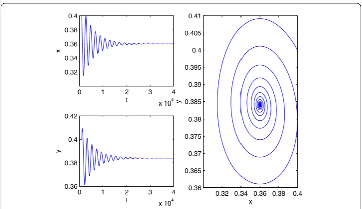
() Whenτ = , from the Routh-Hurwitz criterion, it is obvious thatE∗(., .)is stable. This agrees with Figure .
Figure 1 The trajectories of system (4.1) withτ= 0.The positive equilibriumE3∗is asymptotically stable.
Figure 2 The trajectories of system (4.1) withτ= 0.2.The positive equilibriumE3∗is asymptotically stable.
Now, we will choose two appropriate values ofτto verify. From the discussion of Section , we get
p= ., q= –.,
z∗= ., ω∗= ., τ∗()= ..
(.)
() Whenτ= ., it is obvious thatE∗(., .)is asymptotically stable (see Figure ).
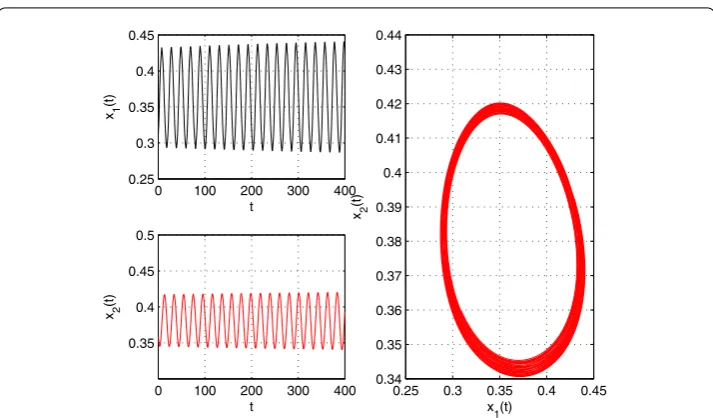
() Whenτ= ., a periodic solution bifurcates from the equilibriumE∗(., .)
Figure 3 The trajectories of system (4.1) withτ= 0.44.A periodic solution bifurcates from the equilibriumE∗3.
From the discussion of Section , we also get a series of data:
c() = –. + .i,
μ= ., T= –., β= –..
Sinceμ> ,β< , the bifurcating periodic solution from the positive equilibriumE∗
is supercritical and asymptotically stable atτ=τ∗(). 5 Conclusion
In this paper, a predator-prey model with a time delay and square root response function is considered. Taking the time delay as bifurcating parameter, the stability of the equi-libria and the existence of Hopf bifurcation is discussed. It is shown that the stability of E∗= (, ) andE∗= (, ) have not changed as the delayτincreases. We have also obtained the conditions at which system (.) undergoes a Hopf bifurcation at the positive equilib-riumE∗. By using the center manifold theory and normal form method, the direction and stability of the Hopf bifurcation are determined. The results of our numerical simulations are in agreement with the theoretical findings.
Acknowledgements
We are grateful to the editors and the anonymous referees for their careful reading and constructive suggestions which lead to truly significant improvement of the manuscript. This research is supported by the National Natural Science Foundation of China (No. 11061016 and No. 11561034).
Competing interests
The authors declare that they have no competing interests.
Authors’ contributions
All authors contributed equally to the writing of this paper. All authors read and approved the final manuscript.
Publisher’s Note
Received: 18 April 2017 Accepted: 21 July 2017 References
1. Zhao, HT, Lin, YP, Dai, YX: Bifurcation analysis and control of chaos for a hybrid ratio-dependent three species food chain. Appl. Math. Comput.218, 1533-1546 (2011)
2. Song, Y, Xiao, W, Qi, XY: Stability and Hopf bifurcation of a predator-prey model with stage structure and time delay for the prey. Nonlinear Dyn.83, 1409-1418 (2016)
3. Zhang, CQ, Liu, LP, Yan, P, Zhang, LZ: Stability and Hopf bifurcation analysis of a predator-prey model with time delayed incomplete trophic transfer. Acta Math. Appl. Sin. Engl. Ser.31(1), 235-246 (2015)
4. Wang, WY, Pei, LJ: Stability and Hopf bifurcation of a delayed ratio-dependent predator-prey system. Acta Mech. Sin.
27(2), 285-296 (2011)
5. Wang, LS, Feng, GH: Stability and Hopf bifurcation for a ratio-dependent predator-prey system with stage structure and time delay. Adv. Differ. Equ.2015, Article ID 255 (2015)
6. Yang, RZ: Bifurcation analysis of a diffusive predator-prey system with Crowley-Martin functional response and delay. Chaos Solitons Fractals95, 131-139 (2017)
7. Yang, RZ, Zhang, CR: Dynamics in a diffusive modified Leslie-Gower predator-prey model with time delay and prey harvesting. Nonlinear Dyn.87, 863-878 (2016)
8. Yang, RZ, Zhang, CR: Dynamics in a diffusive predator-prey system with a constant prey refuge and delay. Nonlinear Anal., Real World Appl.31, 1-22 (2016)
9. Yang, RZ, Liu, M, Zhang, CR: A diffusive toxin producing phytoplankton model with maturation delay and three-dimensional patch. Comput. Math. Appl.73, 824-837 (2017)
10. Salman, SM, Yousef, AM, Elsadany, AA: Stability, bifurcation analysis and chaos control of a discrete predator-prey system with square root functional response. Chaos Solitons Fractals93, 20-31 (2016)
11. Braza, PA: Predator-prey dynamics with square root functional responses. Nonlinear Anal., Real World Appl.13, 1837-1843 (2012)
12. Moreno, M, Platania, F: A cyclical square-root model for the term structure of interest rates. Eur. J. Oper. Res.241, 109-121 (2015)
13. Ajraldi, V, Pittavino, M, Venturino, E: Modeling herd behavior in population systems. Nonlinear Anal., Real World Appl.
12, 2319-2338 (2011)
14. Ruan, SG, Wei, JJ: On the zeros of transcendental function with applications to stability of delay differential equations with two delays. Dyn. Contin. Discrete Impuls. Syst., Ser. A Math. Anal.10, 863-874 (2003)