Consensus templates for protein structure recognition

(1)

C onsensus T em plates for P ro tein

Structure R ecogn ition

Ian Sillitoe

Biomolecular Structure and Modelling Unit

Department of Biochemistry and Molecular Biology

University College London

A thesis submitted to the University of London in the

Faculty of Science for the degree of Doctor of Philosophy

(2)

ProQuest Number: U642775

INFORMATION TO ALL USERS

The quality of this reproduction is dependent upon the quality of the copy submitted. In the unlikely event that the author did not send a complete manuscript and there are missing pages, these will be noted. Also, if material had to be removed,

a note will indicate the deletion.

uest.

ProQuest U642775

This work is protected against unauthorized copying under Title 17, United States Code. Microform Edition © ProQuest LLC.

ProQuest LLC

789 East Eisenhower Parkway P.O. Box 1346

(3)

A b stract

M olecular biology has moved into th e new m illennium w ith th e hum an genome se quenced and publicly available. The challenge now facing th e bioinform atics field is to assign stru ctu re and functional inform ation to protein sequences generated by th is and m any other genomic projects. To m eet this challenge, several stru ctu ral ge nomics initiatives are currently underway w ith th e aim of providing, where possible, a protein stru ctu re w ithin homology m odelling distance for every known sequence. As a result, stru ctu re classification databases will need to provide novel m ethods in order to cope w ith this high infiux of structures.

This thesis presents work on the classification, analysis and recognition of pro tein stru ctu res using th e CATH protein stru ctu re classification database. S tru ctu ral sim ilarity is m easured by com paring contact maps, or th e points of contact between am ino acid residues. By exam ining related structures, it has been possible to identify contacts th a t have been highly conserved during the process of evolution. Protocols to generate accurate m ultiple stru ctu re alignm ents and 3D tem plates based on con sensus contact p a tte rn s found in these alignm ents have been developed. Tem plates have been generated for all homologous superfam ilies in CATH to create a library of unique and identifying ‘fingerprint’ patterns.

These tem plates were applied to the recognition of models generated a t an early stage of ab initio protein stru ctu re prediction. Scanning these early models against a lib rary of tem plates describing conserved contacts allowed the m ost likely superfam ily to be identified. An algorithm was also w ritten th a t perform ed fold recognition using only a lim ited set of contacts w ith the purpose of application to th e early stages of experim ental NM R stru ctu re determ ination.

Finally, th e m ultiple stru ctu ral alignm ents have been used to generate a library of hidden M arkov models (HMMs). These structure-based sequence profiles were thoroughly benchm arked using a strict d ataset of rem ote homologues and appear to outperform other commonly used sequence m ethods.

(4)

A cknow ledgem ents

I would like to take th is o p p o rtu n ity to th a n k all the people who have contributed b o th to my academic research and to my sanity th ro u g h o u t the last four years. I owe a great debt of g ratitu d e to my supervisor C hristine Orengo who has been so generous w ith her tim e, support, and good hum our for th e d u ratio n of my PhD . I would also like to th an k Jan e t T hornton who should take a great deal of credit for her p a rt in m aking the BSM dep artm ent a t UCL such a friendly and stim ulating environm ent to work in.

There are m any people in the dep artm en t th a t I would like to acknowledge and th an k . The first would have to be the CATH F ath er himself. Dr. Jam es Bray. Jam es has done his best to keep me organised (a thankless task) and also on my toes (both scientifically and socially), not to m ention m aking himself personally responsible for me finishing this thesis (m any people, including myself, are sincerely grateful for this). Also, to G abby Reeves, who m ade me porridge when I was w riting this thesis. I have absolutely no idea how you p u t up w ith me for so long b u t m any thanks, especially for laughing so earnestly a t even my m ost appalling jokes. M any thanks also to Daniel Buchan, who has provided an endless stream of entertainm ent and thoroughly useless trivia (see also distraction). S tu a rt Rison and Simon Bergqvist deserve great praise for m anaging to share an office w ith me whilst w riting this thesis. In p articu lar, S tu a rt Rison provided me w ith a m eans of drinking ridiculously strong coffee a t all tim es of th e day and for this I am sincerely grateful.

There are a num ber of other people who have contributed a great deal to th e gen eral atm osphere a t UCL over the years. My th an k s go to th e old crowd; A ndreas Brakoulias, T in a Clarke, Jennifer Dawe, B rian Ferguson, A listair G rant, Andrew H arrison, Thom as “Hot C hocolate” K abir, Frances Pearl, Mike Plevin, Ollie Red- fern, A drian Shepherd and A nnabel Todd. Also to the new crowd: Sarah Addon, Ju an A ntonio, Chris B ennett, Ilhem D iboun, M ark Dibley, A drian EdoUkeh, Stefano Lise and S tath is Sideris.

To th e people who have now left th e lab: I have very much enjoyed my col lab o ratio n w ith Xavier de la Cruz, m ainly due to his ceaseless scientific enthusi asm , b u t also due to th e trips to Barcelona; Andrew M artin, Rom an Laskowski and W illiam V aldar have contributed to my progress in com puter program m ing; also G ail B a rtle tt, R ichard Jackson, Kevin M urray and G ordon W ham ond have all m ade valuable contributions to bo th th e academ ic and social ethos of UCL.

(5)

yond th e call of d u ty in keeping th e com puters and networks in good working order throughout the last 4 years.

To the people who a tte m p ted to keep me sane: A dam Sills, th e infamous duo of Neal H oughton and Neil K erber, Tom K napp and U shm a V ishram , Jack, Mike W illiam s and H arriet and Jon Riches, also to Jam es Garvey and th e rest of UCLU Jitsu Club who have provided excellent stress-relief. Rob and Sally Cray deserve a special m ention for th eir kindness and sup p o rt over the last few years.

M any th an k s also go to th e Palmers: to C arolyn and B ridget for su p po rt and encouragem ent, to Derek for cooking fantastic breakfasts, to Edw ard for trying to explain th e difference between semi-colons and colons (it’s not his fault I d id n ’t listen) and to Joseph for trying to teach me how to play golf (see also tu rf hacking).

My fam ily deserve a huge am ount of credit for offering ju st ab o u t every kind of sup p o rt there is to offer. D uring the last few years my parents have perform ed adm irably as babysitters, taxi-drivers, bank m anagers, w aiters, chefs and wedding organisers. I am very grateful for all th eir support. T hanks also to my sister Claire and her husband Faisal for th eir love and generosity and for accepting the panicked, baby-related early m orning phone calls w ith such good grace. Also, p articu lar thanks go to my G randparents, Stanhope and Joan Blaikley, for th eir constant su p p ort th ro ug h o u t my PhD .

Finally, I would also like to make a very special th a n k you to my long suffering fiancee/wife (depending on when I finish) F m m a Sillitoe. F m has made w riting this thesis possible through her consistent love, su p p ort and (gentle) encouragement. The last person to th an k is my baby daughter Lauren Em ily Sillitoe, who has been of absolutely no help whatsoever in finishing this PhD and I w ouldn’t have it any o ther way.

This work is dedicated to my Nan, Phyllis Sillitoe (1917-2002). She would have read it and said “I t ’s lovely, dear.” (and m eant it).

(6)

C on tents

A bstract

2 A cknowledgem ents

3 C ontents

5 List of Figures

12 List of Tables

16 1 Introduction

17

1.1 P r o t e i n s ... 17

1.1.1 B a c k g r o u n d ... 17

1.1.2 P ro tein S t r u c t u r e ... 18

1.1.3 S tru ctu ral D o m a in s ... 18

1.2 E volutionary R e la tio n s h ip s ... 19

1.2.1 Identifying E volutionary R e l a tio n s h ip s ... 19

1.2.2 Sequence S im ila r ity ... 20

1.2.3 S u b stitu tio n M a tric e s ...20

1.2.3.1 Based on Amino Acid P r o p e r t i e s ... 20

1.2.3.2 Based on Observed M u ta tio n s ... 21

1.2.3.3 Position Specific Score M a tr ic e s ... 22

1.2.4 P ro tein Sequence A lig n m e n t... 23

1.2.4.1 Insertions and D e le ti o n s ... 23

1.2.4.2 Global A lig n m e n ts ...24

1.2.4.3 Local A lig n m e n ts ... 26

1.2.5 Scoring the Sequence A lig n m e n t...27

1.2.5.1 Assessing S tatistical S ig n if ic a n c e ...27

1.2.5.2 Z - s c o r e s ... 27

(7)

Contents

1.2.6 S tru ctural S i m i l a r i t y ... 29

1.2.6.1 Conservation of Sequence and S t r u c t u r e ...29

1.2.6.2 M ethods for E valuating S tru ctu ral Sim ilarity . . . . 29

1.2.7 Structure Com parison A lg o rith m s ... 32

1.2.7.1 Overview of C om parison M e th o d s ... 32

1.2.7.2 Interm olecular S tru ctu re C o m p a ris o n ... 34

1.2.7.3 Intram olecular S tructure C o m p a ris o n ... 37

1.3 P redicting 3D P rotein S tructure from S e q u e n c e ... 42

1.3.1 Background to Protein S tru ctu re P r e d i c t i o n ...42

1.3.2 Homology M o d e ll in g ...43

1.3.3 Fold R e c o g n itio n ... 44

1.3.4 Ab initio Prediction of P rotein S t r u c t u r e ...44

1.4 P ro tein Structure Classification D a t a b a s e s ... 45

1.4.1 Overview of Structure C la ssific a tio n ...45

1.4.2 C A T H ...45

1.4.3 S C O P ...46

1.4.4 O ther S tructure Classification D a t a b a s e s ... 46

1.5 Overview of the T h e s i s ... 48

Inter-R esidue Contacts for Structural A nalysis, Comparison and

Alignm ent

51

2.1 I n tr o d u c tio n ...51

2.1.1 B a c k g r o u n d ...51

2.1.2 Deriving C ontacts from E xperim ental M ethods ... 54

2.1.3 Deriving C ontacts from T heoretical M e th o d s ... 55

2.1.3.1 Prediction of C ontacts from P air P o t e n t i a l s ...55

2.1.3.2 Prediction of C ontacts from C orrelated M utations . . 55

2.1.4 Using a Lim ited Set of D istance C onstraints to Predict 3D S tru ctu re ...56

2.1.5 Aims of this C h a p t e r ... 57

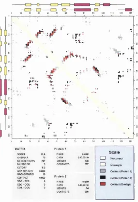
2.2 Analysis and Com parison of C ontact Maps: C O C O P L O T ... 59

2.2.1 Overview ... 59

2.2.2 S tru ctu ral A n a ly s is ... 59

2.2.2.1 C ontact Maps for Single S tr u c t u r e s ... 59

2.2.2.2 Consensus C ontact M aps for M ultiple S tru ctu ral A lig n m e n ts ... 60

(8)

Contents

2.2.3 S tru ctu ral C o m p a ris o n ... 67

2.2.3.1 S tructure-S tructure C o m p a riso n ... 67

2.2.3.2 Structure-T em plate C o m p a riso n ... 69

2.2.4 Extending the Definition of a Consensus C ontact ... 69

2.3 P ro tein S tructure Alignment from C ontact D ata: CONALIGN . . . . 73

2.3.1 Overview ...73

2.3.2 Im plem enting the Double D ynam ic Program m ing A lgorithm . 73 2.3.2.1 Dynam ic Program m ing ... 73

2.3.2.2 Double Dynam ic P r o g r a m m in g ... 74

2.3.2.3 CONALIGN ...74

2.3.3 O ptim isation P r o t o c o l ... 78

2.3.3.1 O v e r v ie w ... 78

2.3.3.2 Scoring S c h e m e s ... 80

2.3.3.3 Sum m ary of O ptim isation Results ... 82

2.3.4 Testing the a lg o rith m ... 84

2.4 D is c u s s io n ...86

G eneration and A pplication of R epresentative Structural Tem

plates for Hom ologous Superfam ilies in CATH

88

3.1 I n tr o d u c tio n ... 88

3.1.1 B a c k g r o u n d ... 88

3.1.2 M ultiple S tructure Alignment A lg o rith m s ... 91

3.1.2.1 S T A M P ...91

3.1.2.2 C O R A ... 93

3.1.3 R epresenting S tru ctu rally Diverse S u p e rfa m ilie s ...95

3.1.4 A i m s ... 97

3.2 M e t h o d s ... 99

3.2.1 M ethods O v e r v ie w ...99

3.2.2 Definitions of E volutionary R e la tio n s h ip s ... 99

3.2.3 G enerating S tru ctu ral T e m p l a t e s ...100

3.2.3.1 Selecting R epresentative S tr u c t u r e s ... 100

3.2.3.2 Selecting S tru ctu rally Coherent S u b - G r o u p s ... 101

3.2.3.3 Building th e S tru ctu ral Tem plates ... 102

3.2.4 O ptim ising the C lustering P r o c e d u r e ... 102

3.2.4.1 Scanning th e Tem plate D a t a b a s e ...104

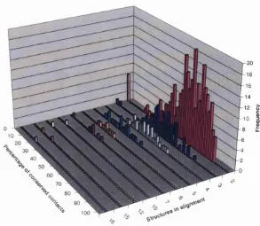
3.2.4.2 Coverage-Versus-Contact P l o t s ... 105

(9)

Contents 8

3.2.5.1 G enerating th e L ibrary of S tru ctu ral Tem plates . . . 107

3.2.5.2 G enerating the D ataset of Rem ote Structures . . . . 107

3.2.5.3 Coverage-Versus-Error P l o t s ...108

3.3 R e s u lts ...110

3.3.1 Overview of R e s u lts ... 110

3.3.2 O ptim ising the S tru ctu ral T e m p l a t e s ...I l l 3.3.2.1 Cytokine superfam ily (1 .2 0 .1 6 0 .3 0 )... I l l 3.3.2.2 Cupredoxin Superfam ily (2.60.40.420) 118 3.3.2.3 a/3-Plait Superfam ily (3 .3 0 .7 0 .3 3 0 )... 122

3.3.2.4 Rossm ann Fold Superfam ily (3.40.50.950) ... 125

3.3.3 Exam ining Pre-Search Filters to Improve Sensitivity and Ac celerate the D atabase Search 128 3.3.3.1 Pre-Search Filter; M inimum Size O v e r l a p ...128

3.3.3.2 Pre-Search Filter: M inim um C ontact Overlap . . . . 128

3.3.3.3 R esults of the Pre-Search F i l t e r s ... 129

3.3.4 Sum m ary of C lustering O ptim isation R e s u lts ... 132

3.3.5 Searching Novel Structures A gainst the Tem plate Library . . . 134

3.4 D is c u s s io n ... 138

3.4.1 Overview ... 138

3.4.1.1 Errors in the Fold Recognition Perform ance of the S tru ctu ral T e m p la te s ... 138

3.4.1.2 D atabase C o m p o s itio n ...139

3.4.1.3 Identification of D istan t S tru ctu ral Sim ilarities . . . 142

3.4.1.4 S u m m a r y ... 143

3.5 A p p e n d i x ... 145

3.5.1 Im plem enting the S tru ctu ral Tem plates in the CATH Server . 145 3.5.1.1 B a c k g ro u n d ...145

3.5.1.2 Using the C RA TH A lgorithm as a R apid P re-F ilter . 145 3.5.1.3 Designing an Interface to th e CATH S e r v e r ... 145

4 Structure Comparison M ethods to Improve

ab in itio

P rotein Struc

ture P rediction

148

4.1 I n tr o d u c tio n ...148

4.1.1 B a c k g r o u n d ... 148

4.1.2 P redicting S tru ctu ral Features from S e q u e n c e ...149

4.1.2.1 Class Prediction ... 150

(10)

Contents 9

4.1.2.3 Inter-Residue C ontact P r e d i c t i o n ...151

4.1.2.4 T ertiary S tructure P r e d i c t i o n ... 152

4.1.2.5 Fold R e c o g n itio n ...153

4.1.3 A i m s ... 154

4.2 M e t h o d s ... 157

4.2.1 Definition of T e r m s ... 157

4.2.2 G enerating th e D a t a s e t s ... 158

4.2.2.1 Sum m ary of D atasets ...158

4.2.2.2 Low Resolution Versions of Native Structures . . . . 158

4.2.2.3 S tructures Predicted by Simons et al. (1 9 9 7 )... 163

4.2.2.4 Predicted Models from C A S P 3 ... 163

4.2.3 Consensus Fold Recognition P r o t o c o l ...167

4.2.3.1 Pairwise C o m p a ris o n ... 168

4.2.3.2 Tem plate C o m p a r is o n ... 168

4.3 R e s u lts ... 171

4.3.1 Overview of R e s u lts ...171

4.3.2 Fold Recognition Using Low Resolution Versions of N ative S t r u c t u r e s ...171

4.3.3 Fold Recognition Using Models from Ab initio S tru ctu re P re diction 177

4.3.3.1 Overview of fold recognition results from ab initio m o d e ls ...177

4.3.3.2 Pairwise C o m p a r is o n s ... 177

4.3.3.3 S tru ctu ral Tem plate C o m p a riso n s...178

4.3.4 Fold Recognition Using Ab initio S tru ctu re Predictions From C A S P 3 ...179

4.4 D is c u s s io n ...180

5 D erivation of Structure-based Sequence M odels to D etect R em ote

Evolutionary R elationships

182

5.1 I n tr o d u c tio n ... 182

5.1.1 B a c k g r o u n d ... 182

5.1.2 Pairwise Sequence A l i g n m e n t ...183

5.1.2.1 Coping w ith Insertions and D e le tio n s ... 183

5.1.2.2 Rigorous Alignm ent A lg o rith m s ... 183

5.1.2.3 F A S T A ... 183

(11)

Contents 10

5.1.3 Profile-based Sequence C o m p a r is o n ... 184

5.1.3.1 B a c k g ro u n d ... 184

5.1.3.2 Hidden Markov Models ...185

5.1.3.3 S A M - T 9 9 ...187

5.1.3.4 P S I-B L A S T ... 187

5.1.4 Interm ediate Sequence S e a r c h i n g ... 188

5.1.5 CATH P ro tein Family D atabase: C A T H - P F D B ... 188

5.1.5.1 Incorporating Genomic Sequences into th e CATH D a t a b a s e ... 188

5.1.5.2 Using th e CA TH -PFD B as an Interm ediate Se quence L i b r a r y ...189

5.1.6 Perform ance of the Sequence Com parison A lg o r ith m s ...189

5.1.7 Structure-B ased Sequence A lig n m en ts... 190

5.1.7.1 Extending the Profile-Based M e th o d s ... 190

5.1.7.2 3 D - P S S M ... 190

5.1.8 A i m s ... 193

5.2 M e t h o d s ...196

5.2.1 Overview of M e th o d s ...196

5.2.2 The SAMOSA Protocol ... 196

5.2.2.1 Overview of the SAMOSA P r o to c o l... 196

5.2.2.2 G enerating the ID-HM M L i b r a r y ... 196

5.2.2.3 G enerating th e 3D-HMM L i b r a r y ... 197

5.2.3 M easuring P e rfo rm a n ce ...198

5.2.3.1 Searching Sequences A gainst th e HMM Libraries . . 198

5.2.3.2 Coverage-Versus-E-value P l o t s ... 200

5.2.4 Selecting D atasets to Test the HMM L i b r a r y ...202

5.2.4.1 G enerating th e Interm ediate Sequence Library . . . . 202

5.2.4.2 Selecting the Benchm ark S e q u e n c e s... 202

5.2.4.3 Q uality Assessment of th e 3D-HMM L i b r a r y ... 202

5.2.4.4 Perform ance of the 3D-HMM L ib r a r y ... 205

5.2.4.5 Coverage-Versus-Error P l o t ... 207

5.3 R e s u lts ... 209

5.3.1 Overview of R e s u lts ... 209

5.3.2 Q uality Assessment of th e 3D-HMM L i b r a r y ... 209

5.3.2.1 Cytokine Four-Helix Bundle S u p e rfa m ily ...210

5.3.2.2 Cupredoxin S u p e rf a m ily ... 211

(12)

Contents 11

5.3.3 Benchm arking the 3D-HMM l i b r a r y ... 215 5.3.3.1 Overview of the Benchm arking P r o c e d u r e ... 215 5.3.3.2 Com parison of Pairw ise and Profile Search M ethods . 215 5.4 D is c u s s io n ... 218

6 D iscussion

221 List of A bbreviations

226

(13)

List o f Figures

1.1 Illustration of stru ctu ral d o m a i n s ... 19

1.2 Chem ical and physical properties of am ino a c i d s ... 21

1.3 Sequence identity m a t r i x ...24

1.4 Flow chart describing the Needleman-W unsch a l g o r i t h m ... 25

1.5 C alculating the Z -s c o re ... 28

1.6 E xtrem e value d is tr ib u tio n ... 28

1.7 Exam ple of high stru ctu ral conservation a t low sequence identity . . . 30

1.8 Exam ple contact m aps for each protein c l a s s ...31

1.9 R oot m ean square deviation ( R M S D ) ... 32

1.10 Interm olecular and intram olecular in te r a c tio n s ... 33

1.11 Rigid body s u p e rp o s itio n ...35

1.12 Flow chart describing the STAMP p r o t o c o l ... 36

1.13 C RA TH stru ctu re com parison a l g o r i t h m ...38

1.14 Flow chart describing the DALI protocol ...39

1.15 Intram olecular stru ctu ral environm ent ... 40

1.16 Flow chart describing the SSAP protocol ...41

1.17 Flow chart providing an overview of th e work discussed in this thesis . 48 2.1 S tru ctu rally diverse relatives from th e ATP G rasp superfam ily... 52

2.2 Exam ple of a contact m ap for a single protein s t r u c t u r e ...60

2.3 Defining a consensus c o n t a c t ... 62

2.4 Exam ple of a consensus co n tact/ alignm ent m a p ... 64

2.5 E xam ple of a consensus distance/ stan d ard deviation p l o t ... 66

2.6 Pairw ise stru ctu re-stru ctu re com parison by overlapping contact m aps 68 2.7 D istribution of percentage of conserved c o n t a c t s ... 70

2.8 D istrib u tio n of percentage of conserved contacts: relaxing th e conser vation c r i t e r i a 72 2.9 Illu stratio n of double dynam ic p r o g r a m m in g ... 76

2.10 Com parison contact m ap based on th e CONALIGN alignm ent . . . . 77

(14)

List o f Figures 13

2.11 Sum m ary flowchart of the CONALIGN optim isation procedure . . . . 80

2.12 R esults from the optim isation score ( 1 ) ... 81

2.13 Illu stratio n of the calculation of global optim isation score ( 2 ) ...82

2.14 R esults from th e optim isation score ( 2 ) ... 83

2.15 R esults from th e sets of reduced contact d a ta ... 85

3.1 S tru ctu ral conservation at low sequence s i m i l a r i t y ...90

3.2 The STAM P a lg o r ith m ... 92

3.3 The CO RA a lg o rith m ...94

3.4 Selecting representative proteins for th e stru c tu ra l t e m p l a t e s ...96

3.5 Flow chart outlining th e work presented in this chapter ...97

3.6 Single and m ultiple linkage c lu s t e r i n g ... 102

3.7 Selecting a reduced d ataset of sim ilar s t r u c t u r e s ... 104

3.8 Exam ple of a coverage-versus-contact p l o t ... 106

3.9 Illu stratio n of the cytokine superfam ily (1.20.160.30) I l l 3.10 Sequence identity versus stru ctu ral sim ilarity plot for th e cytokine superfam ily (1 .2 0 .1 6 0 .3 0 )... 112

3.11 Coverage-contact plots for the cytokine superfam ily (1.20.160.30) . . 114

3.12 Effect of helix shift on consensus contact p a t t e r n ... 115

3.13 Effect of high stru c tu ra l diversity on th e consensus contact m ap . . . 117

3.14 D escription of the supredoxin superfam ily ... 118

3.15 Sequence identity versus stru c tu ra l sim ilarity plot for the cupredoxin superfam ily (2 .6 0 .4 0 .4 2 0 )... 119

3.16 Coverage-contact plots for the cupredoxin superfam ily (2.60.40.420) . 121 3.17 D escription of the o;/3-plait s u p e r fa m ily ... 122

3.18 Sequence identity versus stru c tu ra l sim ilarity plot for th e a/3-plait superfam ily (3 .3 0 .7 0 .3 3 0 )... 123

3.19 Coverage-contact plots for the a/3-plait superfam ily (3.30.70.330) . . . 124

3.20 D escription of a R ossm ann fold s u p e r f a m i l y ...125

3.21 Sequence identity versus stru c tu ra l sim ilarity plot for th e R ossm ann fold superfam ily (3 .4 0 .5 0 .9 5 0 )... 126

3.22 Coverage-contact plots for the Rossm an fold superfam ily (3.40.50.950) 127 3.23 Introducing a m inim um size overlap cutoff as a pre-search filter . . .1 3 0 3.24 Introducing a m inim um contact overlap cutoff as a pre-search filter . 131 3.25 Q uantifying th e coverage-versus-contact plots ...132

(15)

3.27 Perform ance of the stru ctu ral tem plates in recognising topological

re la tio n s h ip s ...136

3.28 R epresentation of sequence families by the stru ctu ral tem plates . . . 140

3.29 Recognition of the d ataset of rem ote homologues in term s of repre sentation in the tem p late lib r a r y ...141

3.30 D istan t stru c tu ra l sim ilarities identified w ith th e stru c tu ra l tem plates 142 3.31 Identification of d istan t stru c tu ra l sim ilarities in the CATH database 144 3.32 R em ote stru c tu ra l assignm ent using th e CATH s e r v e r ... 147

4.1 Overview of the stru ctu re refinement procedure of protein models predicted by ab initio m e th o d s ... 154

4.2 Flow chart for generating high quality ab initio predicted structures . 155 4.3 Exam ple of a fold, or topology, relationship in C A T H ... 157

4.4 Definition of 0i, r and 62 angles... 160

4.5 Simplified model of th e distribution of 61 and 62 angles... 161

4.6 Com parison of RMSD from native for the d ataset of 19 proteins . . . 162

4.7 A fiowchart dem onstrating the consensus fold recognition protocol . . 167

4.8 C om parison contact m aps for native stru ctu re and a predicted model 170 4.9 D istributions of pairwise stru c tu ra l com parison (SSAP) scores . . . . 173

4.10 Recognition rates for pairwise stru c tu ra l com parisons of reduced models 174 4.11 Effect of database com position on fold recognition r a t e s ...176

5.1 Overview of the profile hidden M arkov model ... 186

5.2 Overview of the SAM-T99 protocol for detecting rem ote homologues . 187 5.3 Overview of th e 3D-PSSM p r o t o c o l ... 191

5.4 Overview f lo w c h a r t...194

5.5 Flow chart sum m arising th e SAMOSA p r o to c o l...197

5.6 Flow chart describing the CO RA X plode p r o g r a m ... 199

5.7 Coverage-versus-E-value p l o t ... 201

5.8 Flow chart describing the process of checking the 3 D -H M M s... 204

5.9 G enerating the d ataset of 303 rem ote s e q u e n c e s ... 205

5.10 P lo t of sequence identity against num ber of aligned residues for the non-homologous m a tc h e s ... 206

5.11 P lo t of sequence identity against num ber of aligned residues for the homologous m a t c h e s ...207

5.12 Coverage-versus-E-value plot for th e cytokine four-helix bundle su perfam ily ... 211

(16)

5.14 Coverage-versus-E-value plot for th e a^S-hydrolase superfam ily . . . . 214 5.15 Results of the SAMOSA b e n c h m a rk ... 216

(17)

List o f Tables

1.1 Deriving th e alignm ent from th e traceback p a t h ... 26

1.2 Sum m ary of stru ctu re classification d a t a b a s e s ... 47

2.1 P ro tein relationships as described by Russell & B arton (1994) . . . . 52

2.2 D ataset of stru ctu res used to optim ise CONALIGN param eters . . . . 78

3.1 Sum m ary of th e superfam ilies w ithin th e test s e t ... 103

3.2 Definitions for m easuring perform ance w ith database searching . . . .1 0 9 3.3 Sum m ary of the optim isation results ... 133

4.1 D escription of the 19 structures in the d ataset for low resolution m odelsl59 4.2 D atabase com position for the 19 stru ctu res in the d a tase t for low resolution m o d e l s ...160

4.3 Topology and description of the CASP3 T a r g e t s ... 164

4.4 CASP3 ab initio p r e d ic tio n s ... 165

4.5 D escriptions of ab initio prediction m ethods in C A S P 3 ... 166

4.6 Cases where an analog of the query protein ranked in th e to p position. 175 4.7 R esults when querying the stru ctu re databases w ith ab initio predictions 178 4.8 C om parison of the consensus fold recognition protocol to established th read in g m ethods using CASP3 t a r g e t s ... 179

5.1 Sum m ary of the model d a ta for the cytokine four-helix bundle super fam ily ...210

5.2 Sum m ary of the model d a ta for th e cupredoxin su p e rfa m ily ... 212

5.3 Sum m ary of th e m odel d a ta for the a^-hy d ro lase superfam ily . . . . 213

5.4 C om parison of the results from th e SAMOSA b e n c h m a r k ...217

(18)

C hapter 1

In trod u ction

1.1 P rotein s

1.1.1 B ackground

Proteins form th e basis of alm ost all biological processes (Stryer, 1995). The huge range of functions m ediated by these rem arkable molecules includes catalysis, tra n s po rt, m echanical sup p o rt and molecular recognition. In each case the functional m echanism is closely related to the three-dim ensional stru ctu re of th e protein. Thus, knowledge of th e protein stru ctu re is essential in order to fully u nderstand the mech anism s by which these functions are achieved a t a m olecular level. In addition, u n derstanding th e stru ctu ral basis of these functional mechanisms allows rational drug design to specifically targ et and modify th e behaviour of proteins occurring in either a defective or unw anted biochemical pathway.

As a result of this biological im portance, protein stru ctu re has been th e subject of intense academ ic scrutiny for th e m ajority of the tw entieth century. D uring the early 1930’s, W. T. A stbury dem onstrated th a t hum an hair gave a characteristic X- ray diffraction p a tte rn and th a t this p a tte rn changed dram atically when th e hair was physically stretched (Fundam entals of Fibre S tructure, 1933). In 1951, L. Pauling used these diffraction results to make th e prediction th a t proteins form spring-like CK-helices w ith 3.6 am ino acid residues per tu rn . The use of X-ray diffraction as an experim ental tool in the field of biophysics continued w ith th e first three-dim ensional stru ctu re of th e protein myoglobin reported in 1958 (Kendrew et al., 1958).

At th e end of 2002, the protein d a ta bank (PDB) held th e atom ic co-ordinates of over 19,000 protein stru ctu res determ ined by experim ental techniques such as X-ray crystallography or nuclear m agnetic resonance (NMR) spectroscopy. However, this num ber is alm ost three orders of m agnitude fewer th a n th e num ber of sequences

(19)

Chapter 1. Introduction 18

in th e contem porary sequence databases (the G enB ank nucleic acid datab ase Ben son et al. (1996) contained over 18,000,000 sequence records in November, 2002). E xperim ental stru ctu re determ ination will certainly struggle to keep up w ith the explosion of sequence d a ta from various large-scale genome sequence projects, so it is of great im portance to accelerate these techniques and au to m ate assignm ent of stru ctu re and function from sequence where possible. The challenge facing biolo gists is to discover the function of these proteins individually and how they work in concert to form the biochemical m achinery of life.

1.1.2 P ro tein Structure

In order to u nderstand the principles and features of protein stru ctu re it can be helpful to dissect a typical stru ctu re into its com ponents. P ro tein stru ctu re is often considered in four hierarchical levels of complexity. The first level, called th e prim ary stru ctu re, is the sequential chain of am ino acids, or residues, in the protein. Local regions of this sequence tend towards distinct geom etrical forms such as «-helices, /5-strands and random coil, and are known as secondary stru ctu re elem ents (SSE). These local secondary stru ctu res can be seen to act as a scaffold as they pack together into a global 3D te rtia ry structure, known as th e protein fold. The fourth level of complexity, term ed quaternary structure, describes a collective stru ctu re containing more th an one separate polypeptide chain.

D espite th e alm ost infinite possibilities for conform ations of protein stru ctu re from am ino acid sequence, only a relatively small num ber of stru c tu ra l arrangem ents, or folds, have been observed (less th an 800). In 1992, C hothia proposed there would be “no more th a n 1000 families for the m olecular biologist” (C hothia, 1992). One lim it on the num ber of folds available is of a physical n atu re as there are only a relatively sm all num ber of ways to pack a given set of secondary stru ctu re elem ents into a com pact, globular form (Finkelstein & P titsy n , 1987). An additional reason is th e likelihood th a t all m odern proteins have evolved from a small set of common ancestors.

1.1.3 Structural D om ains

(20)

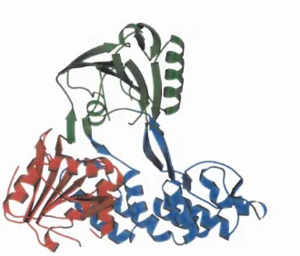
F ig u r e 1.1: MOLSCRIPT (Kraulis, 1991) representations of the three structural domains found in a RNA-helicase protein from Hepititis C virus (PDB structure lA lV , chain A).

domains individually. Nearly half the known globular structures are multidomain, the m ajority comprising two domains, though examples of 3, 4, 5, 6 and 7 domain proteins have also been determined. Structural domains do not always occur in sequential order along the protein chain as a domain can consist of two or more non-local sequence fragments.

1.2 Evolutionary R elationships

1.2.1 Identifying Evolutionary R elationships

(21)

be passed on to sequences for which no an n o tatio n exists.

An evolutionary relationship between two proteins is often dem onstrated by iden tifying a significant sim ilarity between the am ino acid sequences, te rtia ry structures or functional mechanisms of th e proteins. The m easure of significance depends on the confidence required for th e assignm ent of homology, however it is usually based on the likelihood of an equivalent sim ilarity occurring by chance.

1.2.2 Sequence Sim ilarity

A simple m easure of sim ilarity between two protein sequences is the num ber of iden tical residues one sequence shares w ith another, i.e. percentage identity. Sequences sharing more th a n a given threshold value (usually around 30% identity) can be assigned as homologues since it is highly unlikely th a t this degree of sim ilarity could have occurred by chance. However, when th e identity drops below this value it is difficult to assign homology, depending on the size of th e protein (see also section 5.2.4.2). This threshold is commonly referred to as th e ‘Tw ilight Zone’ of sequence sim ilarity (D oolittle, 1986).

Therefore, in order to detect more d istan tly related proteins, i.e. those having less th a n 30% idenities in th eir sequences, sequence alignm ents are often scored according to the num ber of aligned residues th a t share sim ilar properties ra th e r th an identities. The probabilities of residue su b stitu tio n s being accepted and proliferated during protein evolution are sum m arised in su b stitu tio n m atrices.

1.2.3 S u b stitu tio n M atrices

1.2.3.1 Based on Am ino A cid Properties

(22)

Small

P r o lin e

A lip h a tic _s-s

S-H

" r C h a rg ed

' N e g a tiv e Polar

A r o m a tic

Positive

Hydrophobic

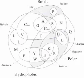
F ig u r e 1.2: A Venn diagram describing the chemical and physical properties of amino acids (Taylor, 1986a). The residues are alanine (A), cysteine (C), aspartic acid (D), glutamic acid (E), phenylalanine (F), glycine (G), histidine (H), isoleucine (I), lysine (K), leucine (L), methionine (M), asparagine (N), proline (P), glutamine (Q), arginine (R), serine (S), threonine (T), valine (V), tryptophan (\V) and tyrosine (V).

1 .2 .3 .2 B a s e d o n O b s e rv e d M u ta tio n s

When comparing two proteins, residue substitution probabilities can be used as a more sensitive assessment of sim ilarity than simple amino acid identity. Thus, accounting for the likelihood of specific amino acid substitutions allows distant evo lutionary relationships to be modelled more accurately.

The likelihood of a given residue substitution can be quantified in a m utation d ata m atrix (MDM). This 2D m atrix describes the probability of each of the 400 potential amino acid substitutions occurring in nature and is based on the observed frequencies of m utations in related sequences. For each amino acid, the 20 sub stitution probabilities are derived by examining a large number of closely related sequences and counting the occurrence of each type of residue substitution.

D ayhofF o r P o in t A c c e p te d M u ta tio n (P A M ) M a tr ic e s

(23)

These alignm ents were global alignm ent, i.e. encom passing the entire length of the sequences. As a result, b o th highly conserved regions and more variable regions were included in b o th the alignm ents and th e subsequent counts of su b stitu tio n frequency.

T he relative su bstitu tio n frequencies were norm alised so th a t the PAM 1 m atrix corresponds to the probability of each residue su b stitu tio n occurring in an evo lutio n ary period of 1 residue m utation every 100 residues. However, considering su b stitu tio n values, based on sequences where only 1 in 100 residues has m utated, will not provide much useful inform ation on d ista n t evolutionary relationships since th e sequences would be alm ost identical. So th e m atrices corresponding to more d istan t relationships are generated by raising each internal value to th e appropriate power, for exam ple giving a PAM 250 m atrix. Due to back m utations (A to B to A) and silent m utations (m utations in the genetic code th a t do not affect th e iden tity of coded am ino acid), the PAM 250 m atrix corresponds to sequences th a t are approxim ately 20% identical.

The Blocks Substitution M atrices (BLO SUM )

T he BLOSUM series of m atrices (Henikoff &: Henikoff, 1992) are generated from local blocks of aligned sequences, rath er th a n full protein sequences, and are taken from the BLOCKS database (Henikoff & Henikoff, 1991). In order to produce m a trices reflecting th e su b stitu tio n probabilities of different evolutionary distances, the sequences used in the alignm ents are first clustered. The sequence iden tity is cal culated for every pair of sequences and any pair w ith a percentage identity above a given threshold are merged together. A series of BLOSUM m atrices have been gen erated using different clustering thresholds to reflect different evolutionary distances (e.g. BLOSOM50 clusters sequences a t 50% identity). These su b stitu tio n m atrices have been seen to outperform the PAM m atrices in searching for a defined set of homologous relationships (Henikoff & Henikoff, 1993).

1.2.3.3 P osition Specific Score M atrices

(24)

This has im plications for identifying the relative im portance of different positions in th e protein sequence based on the analysis of related protein sequences.

By aligning a series of related protein sequences, i.e. by placing equivalent residues in the same vertical rows of the alignm ent, conserved p a tte rn s of residue identity or physicochemical property can often be identified. If a specific am ino acid is seen in a large num ber of sequences th a t are otherwise relatively dissim ilar, then this residue position is likely to correspond to a key role in the protein structure. W hether this key role is due to an active site, or a crucial interaction in th e folding pathway, the highly selective natu re of th e am ino acids identities allowed a t such a position provides inform ation specific to the family of proteins being described. By com bining the probabilities of residue su b stitu tio n s observed a t each position in an alignm ent, a position specific score m atrix (PSSM) can be generated. This can then be used as a unique ‘fingerprint’, or profile, th a t describes the im p o rtan t stru c tu ra l and functional features of a protein family. Profile-based sequence com parisons are discussed in more detail in chapter 5.

1.2.4 P rotein Sequence A lign m en t

1.2.4.1 Insertions and D eletions

Residue su b stitutio n s are not the only mechanisms by which proteins evolve. In sertions or deletions (indels) of sequence fragm ents are also accepted in th e protein stru ctu re. U sually these indels occur in th e variable loops between secondary stru c tu re elements. C om paring two protein sequences therefore requires an alignm ent to be m ade th a t allows for the possibilities of these indels. Residues assigned as equivalent from this alignm ent can then be com pared to calculate a score describing the overall sequence similarity.

In order to provide th e optim al alignm ent of two sequences, it is necessary to consider every possible p erm u tatio n of residues including insertions and deletions. Figure 1.3 shows a 2D m atrix, or dot plot (Maizel JV & Lenk, 1981), com paring th e identities between residues in two protein sequences (labelled A and B). This provides a sim plistic visualisation of the local sim ilarities between the sequences w ith m atching sequence fragm ents corresponding to diagonal lines in the m atrix.

(25)

Sequence A

m 8

c

0) 3

O'

0) W

F ig u r e 1.3: Diagram showing a 2D matrix comparing the identity of each residue in sequence A with the identity of each residue in sequence B.

1.2.4.2 G lo b a l A lig n m e n ts

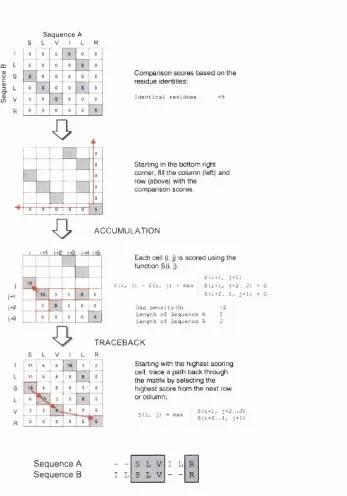
Tlie dynamic programming algorithm is a general m atliem atical procedure th a t can he used to find the o])tiniuni alignment between two sets of data. This algorithm was first applied to align protein setpiences by Needleman and Wtinsch in 1970 (Needleman & Wunsch, 1970) and is still widely used in a variety of bioinformatics techniques. The procedure begins by generating a 2D score m atrix based on the comparison of residues between two protein sequences, A and B. To illustrate, a simple scoring scheme will be used where identical residues are assigned a score of 5 (see figure 1.4).

The dynamic programming algorithm then accumulates these scores, starting with the bottom -right cell in tlie m atrix. To provide each cell with information of the alignment path up to th a t point, the maximum score from the previous row or column startin g from the cell (i + 1, j + 1) can be inherited and added to the comparison score of the cell. Since indels occur less frequently than residue substitutions, a penalty is incurred for inheriting the score from any cell other than

(i + l , j -h 1) as this effectively corresponds to opening a gap in the alignment. The rules of inheritance are formalised in equation 1.1 and the accumulation procedure is illustrated by the third stej) of figure 1.4.

S(i, j) = S{i, j ) + ma x

S ( 2 - b ! , ; + ! )

S{i T 1, j + 2 ..J) 4- G S{i 2 ../, 4 -h 1) -f G

(26)

S e q u e n c e A I

CO L

I:

^ V

1+1

i+a

S I

0 (

. V 1

) 0 £

L R

I 0 0 1

5 () 0 C1 0 0

0 () 5 C1 0 0

a

p

0

' 0

: 1

U Ir - D 1 1 0

1 0

r - | - B - 5

Comparison scores b ased on the residue identities:

Identical residues +5

Starting in the txittom right comer, fill the column (left) and row (atxive) with the comparison scores.

•a

ACCUMULATION

I , i t i , .1+2, jfâ

Each cell (i, j) is scored using the function S(i, j).

S(i, j) = S ( i , j) + max

Sli+1, j + 1) S(i+1, j + 2 . .J) + G S(i + 2. .1, J + 1) + G

Gap penalty(G) -2

Length of S e quence A I Length of Sequence B J

TRACEBACK

S L V 1 L R

1 6 6 16 s T o

L 8 8 6 8 0

S

' I 6 6 B 3 0

L 6 3 5 8

.. 0

V 3 3 K I 0

R 0 0 0 0 0 ^ P s

Starting with the highest scoring cell, trace a path back through the matrix by selectin g the highest score from the next row or column:

S(i, j) S(i+1, J+2..J)

S(i+2..I, j+1)

Sequence A - - _{S L Y} _{I L} _R Sequence B I L S L Y - - R

F ig u r e 1.4: Flowchart describing the Needleman-Wunsch dynamic programming algorithm. This compares each residue in sequence A against every residue in sequence B then finds the optimal global alignment between two sequences.

W here S { i , j ) is the inheritance score of cell i , j (corresponding to residue i of sequence A and residue j of sequence B) and / and J are the lengths of sequences A and B respectively. The gap penalty, G, is given the value -2 for the example in figure 1.4.

(27)

i.e. th e cell from which the inherited score was taken from, are encoded during this accum ulation procedure. Thus, when th e m atrix is fully populated th e highest scoring p a th through th e m atrix can be quickly identified by startin g w ith th e highest score in th e first row or column and traversing back through each inherited cell. The alignm ent between the two sequences can be inferred from the p a th taken by this traceback procedure using the rules described in tab le 1.1. The traceback step and final global alignm ent between the example protein sequences are also shown in figure 1.4.

Traceback from cell (i, j)

Inherited from cell Effect on alignment

(i + i , j + i ) ii + l , j + N j ) (i + N i J + 1)

equivalent residues (no gap) open {Nj — 1) gap in sequence A open {Ni — 1) gap in sequence B

T a b le 1.1: Deriving the alignm ent from the traceback path. This table shows the effect on the final alignment of the three possible cases of inheritance.

1.2.4.3 Local A lignm ents

A global alignm ent algorithm is used to provide the optim al alignm ent between two protein sequences. However, when searching large sequence databases for p utative sequence homologies it is often more im p o rtan t to provide an assessment of ho mology for each sequence comparison, rath er th a n necessarily produce an accurate alignm ent. Also, since m any proteins contain one or more independent stru c tu ra l do m ains (see section 1.1.3), it may be more useful to try to m atch significant fragm ents of protein sequence, ra th e r th a n every residue. If th e query sequence A, com pris ing of a single stru c tu ra l dom ain A i, was com pared against a query sequence B containing two stru c tu ra l dom ains A%, B i, it would only make sense to provide an alignm ent for the m atching dom ain ra th e r th a n th e whole sequence. In th is way, local alignm ents are used to identify sequence sim ilarity between residue fragm ents of two proteins.

(28)

residues + 5, non-m atching residues -1, gap pen alty -2.

= S { i , j ) 4- m a x 0

S{i -f 1, J + 1)

S{i 1.) j 2.. G S[i 2 ..I, j -f-1) -f- G

(1.2)

Since this im plem entation of dynam ic program m ing is designed to align local sequence fragm ents, it was im p o rtan t to elim inate any penalty for startin g a new alignm ent path . Thus, instead of forcing cells to inherit p otentially negative scores from previous paths, an additional choice is included in th e score function S( i ^ j )

which allows the value 0 to be inherited (see equation 1.2).

1.2.5 Scoring th e Sequence A lign m en t

1.2.5.1 A ssessing Statistical Significance

Having found th e optim um alignm ent between two protein sequences, it is im p o rtan t to assess w hether the relationship has occurred as a result of evolution (i.e. descent from a common ancestor) or has arisen by chance. Sequence com parison algorithm s are designed to find the optim al alignm ent between two protein sequences w hether they are related or not. Thus every sequence pair will have sim ilarities sim ply due to the finite num ber of states each residue can occupy. To assign confidence to a pu tativ e homologous m atch, it is necessary to assess w hether th e sim ilarity score is statistically significant. This requires knowledge of which scores to expect simply by chance, i.e. the distribution of the random scores from non-related sequence comparisons.

1.2.5.2 Z-scores

(29)

S-m

s.d

LL

Match Score (S) mean (m)

Sim ilarity S core

F ig u r e 1.5: The typical distribution observed when searching a database with a query sequence. Z-score is calculated by counting the number of standard deviations (s.d) between the matching score (S) to the mean score (m) of the database search.

1.2.5.3 E x p e c ta tio n V a lu es

It has been observed th at the distribution of alignment scores for comparisons be tween random secpiences approximately fits an Extrem e Value D istribution (EVD, Denibo et al. (1994)). Figure 1.6 illustrates the shape of an EVD and quotes the ecpiation used to model this distribution. This equation describes the frequency of finding a sim ilarity score, 5, between two random secpiences of lengths n and m. The values k and A are numerical constants which can be estim ated directly from the database used.

S'

c

0 3 cr 2

LL

Similarity Score (S)

F ig u r e 1.6: Extreme value distribution for pairwise similarity scores (S) between random sequences of length n and rn. The values for k and A are constants derived from the background scores from the database search.

(30)

sim ilarity. However, the probability of a random m atch also depends on the size of the database. In order to take this into account an expectation, or E-value, is calculated. The FASTA sequence com parison algorithm (discussed further in section 5.1.2.3) provides E-values by sim ply m ultiplying the p-value by th e num ber of sequences in th e database, thus providing the significance of a given sim ilarity score while accounting for database size. For example, if a p u tativ e m atch has an E-value of 0.01, it is expected th a t an equivalent sim ilarity score could be found in one out of 100 unrelated sequences simply by chance. The CATH database uses a conservative E-value threshold of 1 * 10“ ^ to signify homology by sequence similarity, i.e. it is highly unlikely th a t this degree of sequence sim ilarity could have occurred by chance.

1.2.6 S tructural Sim ilarity

1.2.6.1 Conservation of Sequence and Structure

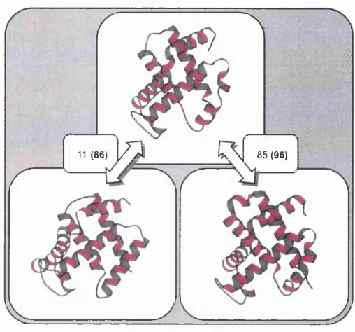
It is well established th a t protein stru ctu re is more conserved th a t protein sequence during the course of evolution (C hothia & Lesk, 1986). Therefore th e protein 3D stru ctu re provides a more sensitive probe of evolutionary relationships th an the am ino acid sequence. This is illustrated in figure 1.7 by m aking two comparisons of stru c tu ra l sim ilarity and sequence identity (based on the stru c tu ra l alignm ent) w ithin three globin-like proteins.

1.2.6.2 M ethods for Evaluating Structural Sim ilarity

D istance P lo ts

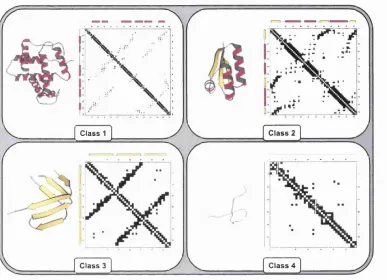
T he earliest and sim plest stru ctu ral com parison m ethods were based on visually inspecting distance plots between proteins. D istance plots, introduced by Phillips in 1970 (Phillips, 1970), are 2D m atrices used to visualise th e distances between residues in a protein stru ctu re and are often shaded according to this distance. The related contact m aps (CM), are used to indicate which residues in a protein stru ctu re are in contact, i.e. w ithin an allowed distance threshold, for example <8Â (see figure 1.8 and chapter 2 for more details). This distance threshold is usually based on the distances between Cq, or Cp atom s of th e am ino acid side chains. W hen these contacts m aps are p lotted in 2D, by shading the cells associated w ith contacting residues, p a tte rn s arise in th e m atrix which often prove characteristic of a p articu lar fold.

(31)

Chapter L Introduction 30

11(86)

\/A

k \ 85(96)

M

i

F ig u r e 1.7: MOLSCRIPT (Kraulis, 1991) representations of relatives from the globin siiperfamily. Pairwise sequence identities are shown for each pair of structures and SSAP structural similarity scores are also given in parentheses. SSAP scores range from 0 up to 100 for identical structures (see section 1.2.7.3).

representing interactions within a-helices which is due to contacts between residues in positions i and i+1 to i+4 (see figure 1.8). Solid lines parallel or anti-parallel to the main diagonal correspond to parallel and anti-parallel ^-sheets respectively. Also, any contact involving an a-helix usually can be recognised by a contact pattern repeating every three or four residues, due to residues being brought into contact by the periodicity of the a-helix (see also section 2.2.2.1).

(32)

Class 1 Class 2

Class 4 Class 3

F ig u r e 1.8; Example contact maps for each protein class, m ainly-a, mainly-/? and mixed-Q /3. Contacts between parallel secondary structures give rise to diagonal lines parallel to the central diagonal. Contacts between anti-parallel secondary structures give rise to lines perpendicular to the central diagonal. Different folds give rise to characteristic patterns in the matrix.

R o o t M e a n S q u a re D e v ia tio n

The root mean square deviation (RMSD) is commonly used as a measure of struc tural similarity between two sets of 3D co-ordinates. The two structures are first superposed so th a t they overlap in 3D space as closely as possible (see section

1.2.7.2), then a set of equivalent residues between the two structures is identified. The distance between each pair of equivalent residues, d*, is then calculated and squared. The sum of these squared distances between equivalent residues is then taken and divided by the number of pairs, N, to give the mean (see equation 1.3).

N

RM SD = \

(33)

In this equation N is the number of equivalent residues identified between the structures and di is the distance between residue i in the first protein and the equivalent residue in the second protein (see figure 1.9).

F ig u r e 1.9: Calculating root mean square deviation (RMSD) as a measure of struc ture similarity following a structural superposition

W hen comparing identical or highly similar proteins, e.g. when analysing con form ational changes on substrate binding, all the residues in the structures may be used for this calculation. However, when considering more distant structural rela tionships it is more common to only calculate the RMSD with respect to C^-atoms th a t are within a specified distance threshold, e.g. <3Â following the structural superposition. When quoting the RMSD it is therefore necessary to provide the number of equivalent residues from which this value was derived. An RMSD of 3Â based on the superposition of 20 residues is far less significant than the same RMSD calculated from 200 residues. As a general rule, proteins of around 150 residues with similar folds would be expected to give a RMSD value of less th an 3.5Â over at least 100 residues.

1.2.7 Structure Comparison A lgorithm s

1.2.7.1 Overview of Comparison M ethods

(34)

been mentioned th a t proteins may share similar structures even when their sequence similarity cannot be distinguished from non-related proteins. Thus, more distant ho mologues may not share sufficient sequence similarity for this initial alignment to be useful, possibly leading the subsequent optim isation procedure to fail to converge on an optim al alignment. The search for a fast and accurate m ethod able to reliably align and compare protein structures has resulted in many different solutions to this problem. A selection of these algorithms are discussed in more detail below.

As with sequence comparison, methods for comparing protein structures com prise two im portant components. The first involves techniques for scoring similari ties in the structural features of proteins. The second is the use of an optim isation strategy th a t can identify an alignment which maximises the stru ctu ral similarities measured.

The m ajority of methods compare the geometric properties of either the sec ondary structure elements or residues along the carbon backbone (Cq or Cp atoms are frequently used). The geometric properties of these residues (or secondary struc tures) are determined from the 3D co-ordinates of the structure deposited in the PDB. Relationship information th a t can be used to describe the structural environ ment within a protein includes, for example, distances or vectors between residues.

IN T E R

%

y V

INTRA

F ig u r e 1.10: Illustration of intermolecular and intramolecular relationships.

(35)

topology of the protein structures being com pared.

S tructure com parison algorithm s can be separated into two distinct categories; those th a t com pare interm olecular relationships and those th a t com pare intram olec ular relationships (see figure 1.10). An example of an interm olecular com parison is a rigid-body superposition m ethod used to calculate RMSD, where co-ordinates of equivalent residues are com pared between structures. In contrast, intram olecular com parison involves the identification of sim ilar internal stru c tu ra l features between proteins, e.g. the com parison of inter-residue contacts.

1.2.7.2 Interm olecular Structure Comparison

Rigid Body Superposition

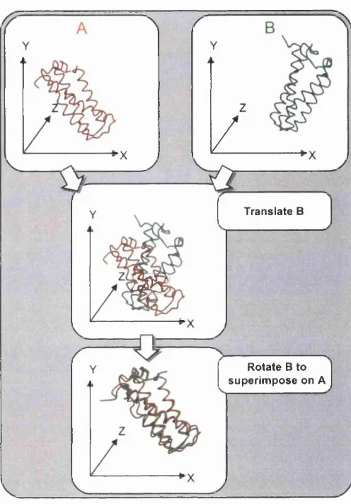
Rossm ann and Argos pioneered rigid body superposition m ethods in the 1970s as the first crystal stru ctu res were being deposited in th e PD B. T heir approaches employed rigid body m ethods to superpose equivalent Cq atom s between protein structures. The m ajor steps of this m ethod can be described as follows:

• Translate b o th proteins to a common position in the co-ordinate fram e of reference.

• R otate one protein relative to the oth er protein, around th e three m ajo r axes.

• M easure th e distances between equivalent positions in the two proteins.

(36)

z

/

X

Translate B

'm

Rotate B to superim pose on A

F ig u r e 1.11: Procedure for finding the optimal rigid body superposition between two protein structures.

is often obtained by manual inspections of the structures or by identifying residues binding common ligands in the active sites of the two proteins.

Once the optim al superposition has been determ ined the difference between the structures is commonly measured by the RMSD. Structures having a similar fold typically give values below 3.5Â, although there is a size dependence to this measure. For example, distant homologues with more than 400 residues may return an RMSD >4.0Â compared to a value of <3.0Â for smaller proteins with less th an 100 residues, but of com parable evolutionary distance.

(37)

as they are independent of protein size and are described in more detail below.

S T A M P

An elegant approach devised by Russell and Barton in their STAMP method (Rus sell & B arton, 1992), used dynamic program ming to refine the set of equivalent residues given by rigid body superposition (see figure 1.12). An initial set of residue pairs is given by a sequence alignment of the proteins and this is used to guide a su perposition of the structures. Intermolecular distances between equivalent residues are then measured and used to score a 2D score or path m atrix, which is analysed by dynamic programming. The resulting path gives a new set of possible equivalent residues. Thus a new superposition can be generated using this refined residue pair set and the path m atrix re-scored and re-analysed to give a b etter path and so on. This is repeated until there is no improvement in the RMSD measured over the equivalent pairs. The m ethod can be summarised as follows:

Score distances between superposed residues in path matrix

A lig n s eq u e n c es

r O

Use dynamic programmingto find best path

S u p e rp o s e s tru c tu re s

Use equivalences given by the best path to re-superpose the structures

J

(38)

• O btain a set of putative equivalent residue positions by aligning the sequences of th e two proteins.

• Em ploy rigid body m ethods to superim pose th e stru ctu res using th is set of equivalent positions.

• Score the 2D m atrix, whose axes correspond to the residue positions in each protein, w ith values inversely proportional to the distances between the super posed residues.

• Apply dynam ic program m ing to determ ine th e optim al p a th through this score m atrix, giving a new set of putative equivalent positions.

Steps 2 to 4 are repeated until there is no change in the set of equivalent residue positions.

1.2.7.3 Intram olecular Structure Comparison

G RATH

One of the sim plest strategies for handling insertions is to discard th e loop regions where insertions are more likely to occur. A num ber of algorithm s have been w ritten th a t employ a m athem atical technique, known as graph theory, to identify equivalent secondary stru ctu re elements (SSEs) between two structures. G raph theoretical approaches to protein stru ctu re com parison were pioneered by A rtym iuk, W illett and co-workers in 1993 (Grindley et ai, 1993). A more recent approach is the GRATH algorithm (Harrison et a i, 2002) which again considers protein structures only in term s of SSEs. Since protein stru ctu res contain approxim ately one order of m agnitude fewer SSEs th an amino acid residues, th is approach drastically reduces th e com plexity of the problem.

(39)

0

d, 0, <D,

chirali _{d, 0, <D,} chirality

d, 0, O, chirality

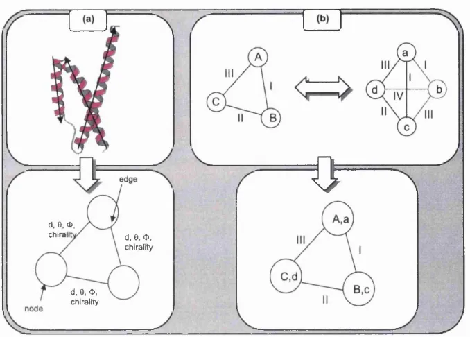
F ig u r e 1.13: The identification of structural similarity with the GRATH algorithm (Harrison et al., 2002). Part (a) describes the procedure for describing a protein 3D structure as a 2D graph based on the relationships between secondary structure elements (SSE). Part (b) illustrates how graph theory is used to identify the maximum sub-graph, or clique, that is common to both graphs representing the proteins being compared.

Since this method aligns SSEs rather than individual residues, it cannot provide an accurate residue-based alignment. However, this algorithm is fast and is able to identify the correct topology within the top 10 matches of a database search 95% of the time. As a result, it can act as perfect filter to generate a list of likely candidates for a more rigorous structural alignment algorithm . The use of GRATH as a pre filter for the assignment of structural relationships in the CATH server is discussed in more detail in section 3.5.1.

D A L I

(40)

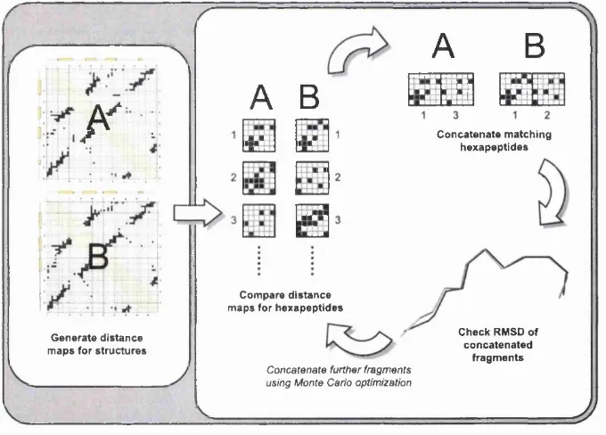
th a t satisfy the constraints on the overall topology and generate a structural unit with an acceptable RMSD. The method can be summarised as follows:

• Divide the protein into hexapeptides and derive the contact map for each hexapeptide.

• Identify hexapeptides whose contact maps match within an allowed threshold, i.e. where there is a similar pattern of distances between equivalent residues.

• C oncatenate matching hexapeptide contact maps to extend the similarity be tween the proteins.

• Superpose the extended fragments and check the difference between the frag ments, as measured by RMSD, is within an allowed threshold, else reject the extension.

Steps 3 and 4 are repeated until no further fragments can be added.

A" :

A B

A

B

H i g

V ¥

‘ ■ 1

G e n e ra te distan c e m a p s fo r s tru c tu res

0

C o m p a re d is ta n c e m a p s fo r h e x a p e p tid e s

Concatenate further fragments using M onte Carlo optimization

C o n c a te n a te m a tc h in g h e x a p e p tid e s

C h e c k R M S D o f c o n c a te n a te d

fra g m e n ts

Consensus templates for protein structure recognition