Considering Product Life Cycle Cost Purchasing Strategy for Solving Vendor Selection Problem s

1

Considering Product Life Cycle Cost Purchasing Strategy

for Solving Vendor Selection Problems

Chien-Wen Shen

Yen-Ting Peng

, Chang-Shu Tu

1_{Department of Business Administration, National Central University}

No.300, Jhongda Rd., Jhongli City, Taiwan, 32001, R.O.C [email protected];

2_{Department of Business Administration, National Central University}

No.300, Jhongda Rd., Jhongli City, Taiwan, 32001, R.O.C. [email protected];

*_{Department of Information Management, Chang Gung University, Taiwan, ROC}

Abstract

The framework of product life cycle (PLC) cost analysis is one of the most important evaluation tools for a contemporary high-tech company in an increasingly competitive market environment. The PLC-purchasing strategy provides the framework for a procurement plan and examines the sourcing strategy of a firm. The marketing literature emphasizes that ongoing technological change and shortened life cycles are important elements in commercial organizations. From a strategic viewpoint, the vendor has an important position between supplier, buyer and manufacturer. The buyer seeks to procure the products from a set of vendors to take advantage of economies of scale and to exploit opportunities for strategic relationships. However, previous studies have seldom considered vendor selection (VS) based on PLC cost (VSPLCC) analysis. The purpose of this paper is to solve the VSPLCC problems considering the situation of a single-buyer-multiple-supplier. For this issue, a new VSPLCC procurement model and solution procedure are derived by this paper to minimize net cost, rejection rate, late delivery and PLC cost subject to vendor capacities and budget constraints. Moreover, a real case in Taiwan is provided to show how to solve the VSPLCC procurement problem.

1. Introduction

Another important issue faced by firms is the vendor selection (VS) problem. The purchasing firm’s preferences or weights associated with various vendor attributes

may vary during different stages of the PLC. Supply professionals must balance their firm’s quality and delivery policies with the cost saving and flexibility profit offered

by vendors, so a vendor’s product manufacturing skills are attractive early on the relationship but efficiency dictates in later stages [7]. The concept of PLC cost (PLCC) originates from the US Department of Defense which are focused on a product’s entire value chain from a cost perspective since the development phase of a product’s life, through design, manufacturing, marketing/distribution and finally

customer services [8].In brief, the PLCC methodology aims to assist the producer to forecast and manage costs of a product during its life cycle. PLCC is a good technique used to assess the performance of a PLC. It can evaluate the total cost incurred in a PLC and assists managers in making decisions in all stages [9]. Elmark and Anatoly (2006) indicated that the PLCC is the total cost of acquiring and utilizing a system over its complete life span [10]. Vasconcellos and Yoshimura (1999) proposed a breakdown structure to identify the main activities for the active life cycle of automated systems [11]. Spickova and Myskova (2015) proposed activity based costing, target costing and PLC techniques for optimal costs management [12]. Sheikhalishahi and Torabi (2014) proposed a VS model considering PLCC analysis for manufacturer to deal with different vendors offering replaceable/spare parts [13]. We integrate VS and PLCC (VSPLCC) procurement planning into a mode for enterprise to reduce their purchasing cost.

reliability, and vendor-area-specific experience. In addition, we would like to maximize the benefit of the procurement process, and must continue to reduce purchasing costs, as well as aiming to achieve minimal cost to obtain the maximum benefit. To help purchasing managers effectively perform and coordinate these responsibilities with their jobs, we need to reconceptualize their role for procurement [14,15]. Schematically, the PLC can be approximated by a bell-shaped curve that is divided into several stages. The PLC is typically depicted as a unit sales curve of a product category over time [7,16].

Narasimhan and Mahapatra (2006) developed a multi-objective decision model that incorporates a buyer’s PLC-oriented relative preferences regarding multiple procurement criteria for a portfolio of products [3]. Life cycle costing is concerned with optimizing the total costs in the long run, which consider the trade-offs between different cost elements during the life stages of a product [17]. Their research aims to obtain a comprehensive estimation of the total costs of alternative products or activities in the long run. It is usually possible to affect the future costs beforehand by either planning the use of an asset or by improving the product or asset itself [18]. Previous studies, however, have seldom examined the VSPLCC procurement problem in the situation of single-buyer-multiple-supplier.

The paper is organized as follows. We review the literature regarding the quantitative methods for the VS decision in Section 1. Section 2 presents the formulations and solutions to the VSPLCC procurement problem using both MOLP and MCGP approaches. In Section 3, the solution procedures of the two approaches for VSPLCC procurement problem are presented based on the modified dataset of the auto parts manufacturers’ example and a numerical example is adopted from a light-emitting diode company in Taiwan [19]. In Sections 4 discussions of MOLP and MCGP are provided, conclusions regarding the advantages of solving the VSPLCC procurement problem in the four stages of the PLC with MOLP and MCGP approaches are addressed in Sections 5.

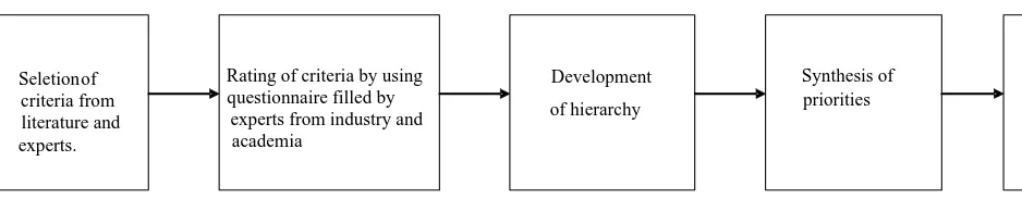
Please insert Figure 1 here

2.

The VSPLCC Procurement Approaches

2.1 Linear Programming Technique

MCGP method which allows one goal mapping multiple aspiration levels to find the best achievement levels for multiple objective decision making (MODM) problems [27, 28]. Accordingly, in order to improve the quality of decision making for solving the VSPLCC problem, we integrate AHP and MCGPmethods, wherein both qualitative and quantitative issues are considered for more realistic VSPLCC applications. The AHP-MCGP method is also used to aid decision makers (DMs) in obtaining appropriate weights and solutions for the VSPLCC problem. The proposed VSPLCC model can be easily used to select an appropriate vendor from a number of potential alternatives. The framework adopted for this study is shown in Figure 1.

The formulation of the VSPLCC model requires the following assumptions, indices, decision variables and parameters.

2.2 Fuzzy Multi-Objective Models for the VSPLCC Procurement

Problem

(i) Only one item is purchased from each vendor. (ii) Quantity discounts are not considered.

(iii) No shortage of the item is allowed for any of the vendors.

(iv) The lead time and demand for the item are constant and known with certainty. The sets of indices, parameters, and decision variables for the VSPLCC model are listed in Table 1.

2.3 VSPLCC Procurement Model

The multi-objective VSPLCC procurement problem with four fuzzy objectives and some constraints are as follows:

Min Z1t     n i t it itX P 1 4 4

~ _{the total net cost (1)}

Min Z2t Q X_it

n

i t it

  

 1 4

1

~ _{therejects items for vendor i (2)}

Min Z3t L X_it

n

i t it

  

 1 4

1

~ _{the late delivered items for vendor i (3)}

Min Z4t C X_it

n

i t it

  

 1 4

1

the product life cycle cost for vendor i (4)

The following constraints are given for the VSPLCC procurement problem:

D X t n i t it ~ 1 4 1  

  (aggregate demand constraint) (5)

U

Xit ~it i = 1, 2,…, n, t = 1, 2, 3, 4, (capacity constraint) (6)

p X

r it it

n

i t

it 

 

 1 ( ) 4

1

; t = 1, 2, 3, 4, (total items purchasing constraint) (7)

F X

f it it

n

i t it

  

 1 ( ) 4

1

; t = 1, 2, 3, 4, (quota constraint) (8)

B X

Pit it it; i = 1, 2,…, n, t = 1, 2, 3, 4, (budget constraint) (9)

0 

Xit , i = 1, 2,…, n, t = 1, 2, 3, 4. (non-negativity constraint) (10)

such as the AHP with a geometric mean (see details of the process in Chakraborty, Majumder; Sarkar, 2005) [32].

2.3 The Solution of the VSPLCC Procurement Problem Using the

Weight Additive Approach

In this section, we present the general multi-objective model for solving the VS problem. To specify the weights of the goals and constraints in a fuzzy environment, we can use a fuzzy approach, instead of having the DM subjectively assign values to these weights. To obtain the supertransitive approximation of the previous comparison matrix, we construct supplementary matrices A1, A2,…, An. The jth row of matrix Aj is the same as the jth row of the initial matrix A, where the supplementary matrix

 





 and each row of the matrix Aj is computed as follows (_T＊:

Transpose): a aj,

j

j  ( 1) ,

1 1 a j a

a jj

j 

. ) ( ,..., )

( 1 .

2 1

2 a j a a a jn a

a jj

j n j j

j   

 Next, we

construct the supertransitive approximation, _{As a}s ,

ij

 i , j = 1, 2, …, n, by taking

the geometric mean of the corresponding elements from the supplementary matrices

A1_{, A}2_{,…, A}n_{. More formally, (} 1 2 _{... )}1 a a

a

a ij ij nij n

s

ij    . Then we obtain the largest

value of As _{with an eigenvector method. The corresponding eigenvector is the optimal}

weight for the criteria [26,33]. In the solution to the VSPLCC problem model, the AHP with weighted geometric mean (WGM) is calculated using a supertransitive approximation. Thus these weights are assigned separately. In these equations, jt is

the weighting coefficient that shows the relative importance at the four stages of the PLC.

Model 1: The weighted additive (WA) approach [34], which is formulated as follows:

Max  * 1

4

1

jt s

j t jt

 

  (11)

s.t

), (x

zjt jt 

  j = 1, 2,… , q, t =1, 2, 3, 4, (12)

), (x

hrt rt 

  r = 1, 2,…, h, t =1, 2, 3, 4, (13)

, )

(x b

gmt  mt m =1,…, p, t =1, 2, 3, 4, (14)

 

t , t =1, 2, 3, 4, (15)

 

 

s

j t jt

1 4

1

=1,jt0, t =1, 2, 3, 4, (16)

, 0 

xnt n = 1, 2,…, i, t =1, 2, 3, 4. (17)

See Amid et al. (2011) [35] for a more detail.

2.4 The Solution of the VSPLCC Procurement Problem Based on Lin’s

Weighted Max-Min Approach

Lin (2004) proved that a weighted max-min (WMM) approach could find an optimal solution such that the ratio of the achievement level approximates the ratio of the weight as closely as possible [41]. He noted that the WA model gives heavier weights to objectives of higher achievement levels than do others models. However, the ratio of the achievement levels is not necessarily the same as that of the objectives’ weights [35, 36]. Thus, to obtain the solution of the VSPLCC problem model, WMMmodel is used as follows:

Model 2: Lin’s WMM approach (Lin, 2004) [36]:

Max t, (18)

), (x

hrt rt 

  r = 1, 2,…, h, t =1, 2, 3, 4, (20)

, )

(x b

gmt  mt m = 1,…, p, t =1, 2, 3, 4, (21)

 

t , t = 1, 2, 3, 4, (22)

    s j t jt 1 4 1

=1, jt0, t =1, 2, 3, 4, (23)

, 0 

xnt n = 1, 2,…, i. t =1, 2, 3, 4. (24)

2.5 The Solution of the VSPLCC Procurement Problem Based on

MCGP Approaches

In real decision-making problems, goals are often interrelatedin which DMs can set more aspiration levels using the idea of multi-choice aspiration level (MCAL) to find more appropriate resources so as to reach the higher aspiration level in the initial stage of the solution process Chang (2007) [27]. To address this issue, the MCGP AFM models are developed below.

Model 3: The MCGP AFM (achievement function model) (case Ι) is used in the case of “the more, the better” as follows.

Minimize  





      n i t it it it it it

it d d e e

w 1 4 1 ) ( ) ( 

s.t. fti X bitditdit bity_it

  )

( , i = 1, 2, …, n, t = 1, 2, 3, 4, (25)

g e e

yit it it  _it,max

 

, i =1, 2,…, n, t = 1, 2, 3, 4, (26)

g y

g_it,min  _it _it,max, i = 1, 2,…, n,t = 1, 2, 3, 4, (27)

, 0 , , ,     e e d

dit it it it i = 1, 2,…, n, t = 1, 2, 3, 4. (28)

XF where F is a feasible set and X is unrestricted in sign.

where bit  {0, 1} is a binary variable attached to f_it(X)y_it, which can be either

appropriate constraints according to real needs.

Model 4: The MCGP AFM (case II) is used in the case of “the less, the better” as follows.

Minimize  





      n i t it it it it it

it d d e e

w 1 4 1 ) ( ) ( 

s.t. fti X bitditditbityit

  )

( , i = 1, 2,…, n, t = 1, 2, 3, 4, (29)

g e e

y_it _it _it _it,max, i = 1, 2,…, n, t = 1, 2, 3, 4, (30)

g y

g_it,min  _it _it,max, i = 1, 2,…, n, t = 1, 2, 3, 4, (31)

, 0 , , ,     e e d

dit it it it i = 1, 2,…, n, t = 1, 2, 3, 4. (32)

where all variables are defined as in model 3. The mixed-integer terms Eqs.(29) and (32) can easily be linearized using the linearization method (Chang, 2008) [28]. As seen in Eqs.(25), (29), (30) and (31), there are no selection restrictions for a single goal, but some dependent relationships exist among the goals. For instance, we can add the auxiliary constraint _bit _bi1,t_bi2,t to the MCGP AFM, where bit, bi1,t

and bi2,tare binary variables. As a result, bi1,t or bi2,t must equal 1 if bit = 1.

This means that if goal 1 has been achieved, then either goal 2 or goal 3 has also been achieved.

2.6 The Solution Procedure of VSPLCC Procurement Problem

In order to solve the VSPLCC problem, the following procedure is then proposed.

Step 1: Construct the model for VSPLCC procurement.

Step 2: A WGM technique is used to determine the criteria for MOLP model [37]. A WGM technique with a supertransitive approximation is used to obtain the

Step 3: Calculate the criteria of weighted geometric mean for solving VSPLCC problem.

Step 4: Repeat the process individually for each of the remaining objectives. It determines the lower and upper bounds of the optimal values for each objectives corresponding to the set of constraints.

Step 5: Use these limited values (see Table 3) as the lower and upper bounds for the crisp formulation of the VSPLCC problem.

Step 6: Based on steps 4-5 we can find the lower and upper bounds corresponding to

the set of solutions for each objective. Let Zjt and Zjt denote the lower

and upper bound, respectively, for the jt th objective (Zjt) (Amid, Ghodsypour; O’Brien, 2011) [35].

Step 7: Using the weighted geometric mean with a supertransitive approximation to solve Model 1 by following Eqs. (11) to (17).

Step 8: Formulate and solve the equivalent crisp model of the weighted geometric mean max-min for the VSPLCC problem to solve Model 2 by following Eqs. (18) to (24).

Step 9: Use the weighted geometric mean and the no-PW (penalty weights) formulation of the fuzzy optimization problem to solve Model 3 by following Eqs. (25) to (28).

Step 10: Formulate Model 4 using the weighted geometric mean and the PW formulation of the fuzzy optimization problem by following Eqs. (29) to (32). Assume that the purchasing company manager sets a PW of five for a vendor

Step 11: The four stages of the PLC cost matrix are given as follows (Demirtas; Ustun, 2009) [37]:           56 . 3 05 . 3 52 . 3 94 . 3 00 . 1 86 . 0 92 . 0 04 . 1 82 . 1 23 . 1 52 . 1 92 . 1

Step 12: Assume that the four stages of the PLC budget matrix are given as follows:

          200 , 35 500 , 37 000 , 36 000 , 35 000 , 110 000 , 125 000 , 120 000 , 100 000 , 26 400 , 27 500 , 26 000 , 25

Step 13: Solve the MOLP and MCGP models for the fuzzy optimization problem. Step 14: Analyze the PLCCs and capacity limitations for the four stages. The

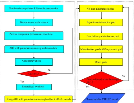
procedure of the VSPLCC problem-solving model is illustrated through a numerical example. Figure 2 shows the use of the AHP with a WGM and supertransitive approximation with a WGM technique to the MOLP and MCGP approach models are used to solve VSPLCC problems.

Please insert Figure 2 here

3. Numerical Example

As global warming intensifies and carbon dioxide emissions are important issues in the warming caused by greenhouse gases. Reducing the greenhouse effect and protecting the Earth's environment are import goals associated with the use of white light-emitting diodes (LED) since they consume substantially less electrical power than other light sources. White-light LED power can reduce the amount of crude oil used in power plants and substantially reduce the generation of CO2 emissions, which

tons of CO2 annually.

We use the VSPLCC procurement model solve a real case in the distribution department for the Everlight Company (the leading LED manufacturer in Taiwan), which is part of a multi-national group f o r LED research and development (R&D) sector. External purchases account for more than 75% of the total annual costs, and the firm works on a make-to-order basis. The company’s management aimed to improve the efficiency of the purchasing process and reconsidering the company’s sourcing strategies. A manager felt that the company must evaluate and certify the company’s vendors to ensure reductions in product inventory and time to market. The company sought to develop longer-term, trust-based relationships with a smaller group of vendors, and the company manager appointed a team to recommend three or four suitable vendors. This team consisted of several managers from various departments, including purchasing, marketing, quality control, production, engineering and R& D. The members of the team organized several meetings to create profiles for the competing vendors and constructed an initial set of three vendors for evaluation purposes. A VSPLCC procurement model is then developed to select the appropriate vendors and to determine their quota allocations in uncertain environments.

The team considered some objective functions, and constraints as follows: minimizing the net cost, minimizing the net rejections, minimizing the net late deliveries, minimizing the PLC cost, vendor capacity limitations, vendor budget allocations. The other considerations were: price quoted (Pi in $), the percentage of

rejections (Ri), the percentage of late deliveries (Li), the PLCC (Ci), the PLC of the

vendors’ capacities (Ui), the vendors' quota flexibility (Fi, on a scale from 0 to1), the

(Bi) were also considered.

The least amount of flexibility in the vendors’ quotas is calculated as Q = FD and the smallest total purchase value is calculated as P = RD. If the overall flexibility (F) is 0.03 on a scale of 0–1, if the overall vendor rating (R) is 0.92 on a scale of 0–1 and if the aggregate demand (D) is 20,000, then the least amount of flexibility in the vendors’ quotas (F) and the smallest total purchase value of the supplied items (P) are 600 and 18,400, respectively. The three vendor profiles are shown in Table 2.

Please insert Table 2 here

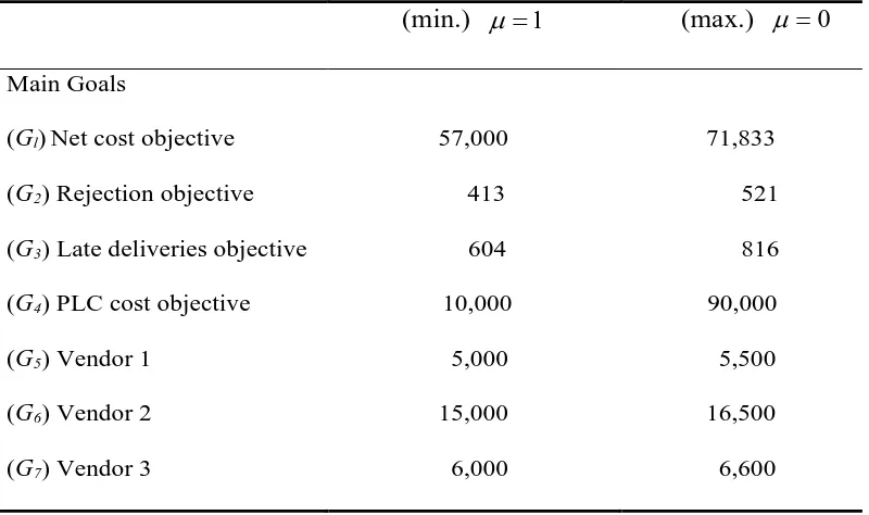
In this case, the linear membership function is used to fuzzify the right-hand side of the constraints in the VSPLCC problem. The values of the uncertainty levels for all of the fuzzy parameters were taken as 10% o f the corresponding values o f the deterministic model. The datasets for the values at the lowest and highest aspiration levels of the membership functions are given in Table 3 .

Please insert Table 3 here

3.1 Application of the WA Approach to the Numerical Eexample

We obtained the solution using the WA approach of Tiwari et al. (1987) and in the next section we show the procedure by using the WGM AHP to construct a WGM supertransitive approximation to obtain the binary comparison matrixes.

3.1.1 Using the

WGM

AHP Process to Solve the VSPLCC Procurement

Problem

considered and may include man y judgmental factors [39,24,40]. Please insert Figure 3 here

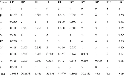
These criteria are shown in Figure 3. The VSPLCC problem addresses how optimally performing vendors can be selected given the desired criteria.The AHP is one of the most widely used MCDM methods it can be used to handle multiple criteria. The criteria for the VS problem are shown in Table 4. Based on the ratings obtained using the questionnaire, the average matrix is shown in Table 5. The maximum value of the eigenvector for the above matrix max is 10.77 [32]. The consistency index C.I. is

given by (max-n)/ (n-1) = 0.09. The random index for the matrix of order 10 [41]. R.I. is 1.49. The consistency ratio C.R. is given by C.I. / R.I. = 0.06, which is not greater than 0.1(<0.1 acceptable).

Please insert Tables 4-6 here

A

=



1 6 4 9 3 4 9 9 8 2

1 / 6 1 1 / 2 3 1 / 3 1 / 3 2 4 5 1 / 4

1 / 4 2 1 4 1 / 2 1 / 2 3 5 6 1 / 3

1 / 9 1 / 3 1 / 4 1 1 / 5 1 / 2 2 3 3 1 / 6

1 / 3 3 2 5 1 1 4 6 7 1 / 2

1 / 4 3 2 5 1 1 4 6 7 1 / 2

1 / 9 1 / 2 1 / 3 2 1 / 4 1 / 4 1 3 4 1 / 5

1 / 9 1 / 4 1 / 5 1 / 2 1 / 6 1 / 6 1 / 3 1 2 1 / 8

1 / 8 1 / 5 1 / 6 1 / 3 1 / 7 1 / 7 1 / 4 1 / 2 1 1 / 9

1 / 2 4 3 6 2 2 5 8 9 1

                               

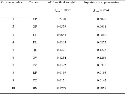
The AHP process with a geometric mean was applied to this comparison matrix, and the following weights were obtained [53]: w1 = 0.2958, w2 = 0.0579, w3 = 0.0863,

w4 = 0.0365, w5 = 0.1291, w6 = 0.1254, w7 = 0.0392, w8 = 0.0199, w9 = 0.0151,and w10

= 0.1949 (see Section 4.1.1: Using the AHP process with a geometric mean).

using the following algorithm described in Section 3.2: Solution to the VSPLCC problem via the WA approach. The ten supplementary matrices corresponding to A are: A=                                 1 9 8 5 2 2 6 3 4 7231 . 0 1111 . 0 1 5 . 0 25 . 0 1429 . 0 1429 . 0 3333 . 0 1667 . 0 2 . 0 0509 . 0 125 . 0 2 1 3471 . 0 1667 . 0 1667 . 0 5 . 0 2 . 0 25 . 0 0647 . 0 2 . 0 4 8808 . 2 1 3333 . 0 25 . 0 1 2805 . 0 5 . 0 1153 . 0 5 . 0 7 6 3 1 1 5 2 3 3868 . 0 5 . 0 7 6 0903 . 4 1 1 5 7579 . 0 3 4363 . 0 1667 . 0 6161 . 1 3 2192 . 0 3789 . 0 2 . 0 1 25 . 0 3333 . 0 1082 . 0 3333 . 0 2701 . 4 6239 . 3 3 5 . 0 5 . 0 4 1 4902 . 1 2917 . 0 25 . 0 5622 . 4 4 2 3333 . 0 3333 . 0 3 6711 . 0 1 1958 . 0 3830 . 1 6386 . 19 4672 . 15 6768 . 8 5851 . 2 2919 . 2 2397 . 9 4278 . 3 1080 . 5 1

The supertransitive approximation method [54] was applied to this comparison matrix, and the following weights were obtained: w1 = 0.3020, w2 = 0.0611, w3= 0.0810, w4

=0.0272, w5 = 0.1226, w6 = 0.1294, w7 = 0.0376, w8 = 0.01936, w9 = 0.0142,and w10 =

0.2057 and its corresponding eigenvalue max is 9.94. [33]. Table 6 shows the AHP

method weight with geometric mean and the supertransitive approximation with the

geometric mean. For this VSPLCC problem, we obtained the optimal quota allocations

(i.e., the purchasing order), vendor product capacity limitations, and the budget constraints of the different vendors by using the WA approach model (i.e., model 1) in accordance with Eqs. (11) to (17).

3.2 Using Lin’s WMM Approach to Solve the Numerical Example

For this VSPLCC illustrative example, we obtained the optimal quota allocations (i.e., the purchasing order) subject to vendor product capacity limitations, and budget constraints among the different vendors with Lin’s WMM [36].

3.2.1 Using a MCGP AFM (model 3: case Ι) to Solve the Numerical

Example

For this VSPLCC procurement problem, we obtained the optimal quota allocations (i.e., the purchasing order), supplier product capacity limitations and budget constraints among the different vendors by using the MCGP method and a no-PW approach (according to Eqs. (25) to (28)). This VSPLCC problem was then formulated as follows (using the first stage of the PLC for Model 1):

Max = 0.29581+ 0.05792+ 0.08633+ 0.03654 + 0.12915+ 012546+

0.03927+ 0.01998+ 0.01519+ 0.194910

Main Goals:

)

(G11 3x112x216x31= 57,000 (G11, MIN.) or 71,833 (G11, MAX.),

)

(G21 0.05x110.03x210.01x31= 413 (G21 ,MIN.) or 521 (G21 ,MAX.),

)

(G31 0.04x110.02x210.08x31= 604 (G31 ,MIN.) or 816 (G31 ,MAX.),

)

(G41 1.92x111.04x213.94x31=10,000 (G41 ,MIN.) or 90,000 (G41 ,MAX.).

Capacity Constraints Goals:

)

(G51 x11= 5,000 (G51 ,MIN.) or 5,500 (G51 ,MAX.) (X11, Vendor 1’s product capacity),

)

(G61 x2115,000(G61 ,MIN.) or 165,000(G61 ,MAX.) (X21,Vendor 2’s product capacity),

)

(G71 x316,000(G71 ,MIN.) or 165,000(G7 1,MAX.) (X31, Vendor 3’s product capacity),

000 , 20 31 21

11x x 

x

Budget Constraints Goals:

)

(G81 3x1125,000(G81 ,MIN.) or 27,500 (G81 ,MAX.) (X11, Vendor 1’s budget constraint),

)

(G91 2x21100,000 (G91 ,MIN.) or 110,000 (G91 ,MAX.)(X21, Vendor 2’s budget

constraint),

)

constraint).

3.2.2 Using a MCGP AFM (model 4: case II) to Ssolve the Numerical

Example

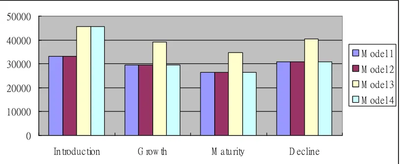
The subjectivity inherent to the determination of both the desired level of attainment for each goal and the penalty weights assigned to deviations from the goal may present a problem [19,36]. Suppose that the purchasing company’s manager sets a penalty weight of five for the vendor missing the net cost goal, four for missing the rejection goal, three for missing the late deliveries goal, and two for exceeding the PLC cost goal [28]. For this VSPLCC problem, we obtained the optimal quota allocations (i.e., the purchasing order), supplier product capacity limitations and budget constraints among the different vendors using the MCGP method and a PW approach in accordance with Eqs.(29) to (32). After using MOLP and MCGP approaches to solve the VSPLCC problem at the four stages of the PLC, we summarized the results of the problem in Tables 7 to 15. From Z4t (i.e., the PLC cost

goal) of Figure 4, we can see that the maturity stage has the lowest PLC cost, in contrast the growth and decline stages have similar costs and the introduction stage has a high PLC cost.

Please insert Tables 7-12 here

Please insert Figure 4 here

4. Discussion of the Results of the Two Types of MOLP and MCGP

Model Approaches

After solving the VSPLCC procurement problem

,

approach have the same results in the first stage of the PLCs. With regards to the MCGP approaches with the geometric mean (no-PW restrictions), x11 = 5,000 (due to

the absence of PW constraints), b11=1 and b51 =1. The forced bound order quantity of

vendor 1 was 5,000 (i.e., for model 3 at the first stage (Introduction), x11=5,000) (see

Tables 7 and 11). With regards to the other approaches (i.e., the MCGP approach with the geometric mean and the PW approach), b12=1 and b62 =1. The forced bound order

quantity of vendor 2 was greater than 15,000 (i.e., for model 4 at the second period (Growth), x22=15,750). To guarantee the net cost goal, the rejection goal or the late

delivery goal, zero value should be achieved (e.g., if b12 =1 and b62 =1, then forces bit equal to zero used to adjust the purchasing quantity) (see Tables 8 and 12). We found the MCGP model to be stable with regard to the PLCC in all of the stages (see Tables 13-15).

Please insert Table 13 here

Please insert Table 14 here

Please insert Table 15 here

Based on the solutions to the two type’s goal-programming models, we found that the MCGP model demonstrated more stable control of the PLC cost over all of the stages. We also found that the weighted geometric mean with AHP and PW methods have good control conditions for constructing an MCGP model (model 4) withinfour stages.

5. Conclusions and Managerial Implications

The results obtained using the MOLP and MCGP approaches for determining

known with certainty. The effectiveness of the VSPLCC procurement model was

demonstrated with a real-world problem adopted from a leading LED company in

Taiwan. Managers in high-tech companies can easily apply our proposed model to

select their vendors in a fuzzy environment using the MOLP and MCGP approaches.

Some managerial implications are found as follows: (i) Doing so is practical

because the no-PW and PW MCGP model approaches (MCGP AFM models 3 and 4)

do not require precise knowledge of all of the parameters and they make the

application of a fuzzy methodology more understandable [35,27,28], (ii) the No-PW

and PW MCGP models are demonstrated more stable over all of the PLC stages, and

(iii) company managers can easily use MOLP and MCGP approaches to solve

VSPLCC procurement problems. In addition, integrating other mathematical models,

such as the Pareto concept with AHP [43], ANP [37] with DEAHP [44], or AHP-QFD

[45] with the MOGP [46] and MCGP [27,28,47] models to solve the VSPLCC

problems in a multi-item/multi-vendor environment that can be performed in

conjunction with the various models [48].

Author Contributions: Conceptualization, P.Y.T. and S.C.W; formal analysis, T.C.S and P.Y.T.; writing—original draft preparation, T.C.S and P.Y.T.; writing—review and editing, T.C.S and P.Y.T.; supervision, S.C.W

Funding: This research received no external funding.

References

1. Hsu, P.H.; Teng, H. M.; Jou, Y.T.; Wee, H. M. Coordinated ordering decisions for products with short lifecycle and variable selling price. Comput. Ind. Eng. 2008, 54, 602–612.

2. Wen, Z.K.; McClurg, T. Coordinated ordering decisions for short life cycle products with uncertainty in delivery time and demand.Eur. J. Oper. Res. 2003, 151, 12–24.

3. Narasimhan, R.; Talluri, S.; Mahapatra, S. K. Multiproduct, multicriteria model for supplier selection with product life-cycle considerations. Decision Sciences, 2006, 37 (4), 577–603.

4. Rink, D.R.; Dodge, H.W. Industrial sales emphasis across the life cycle. Ind. Market Manag.1980, 9 (4), 305–310.

5. Wong, H.K.; Ellis, P.D. Is market orientation affected by the product life cycle? J. World Business, 2007, 42 (2), 145–156.

6. Rink, D. R.; Fox, H. W. Coordination of procurement activities withdemand: an expanded conceptual model. Innovative Marketing, 20117 (1),78–87 7

.

using integrated multi-criteria decision-making methodology. International Journal of Production Economics, 2004, 91, 1–15.

8. Perng, C.; Lyu, J.J.; Lee, J.P. Optimizing a collaborative design chain by integrating PLC into SSDM. Int. J. Elect. Bus. Manag. 2013, 11, 88–99. 9. Hatch, M.; Badinelli, R.D. A concurrent optimization methodology for

concurrent engineering. IEEE T. Eng. Manage. 1999, 46, 72–86.

11. Vasconcellos, N. M.; Yoshimura, M. Life cycle cost model for acquisition of automated systems.Int. J. Prod. Res.1999, 37(9), 2059–2076.

12. Spickova,M.; Myskova, R. Costs efficiency evaluation using life cycle costing as strategic method.Bus. Econo. Manag. 2015, Conference, BEM2015.

13. Sheikhalishahi, M.; Torabi, S.A. Maintenance supplier selection considering life cycle costs and risks: a fuzzy goal programming approach. J. Oper. Res. Soc.2014, 52, 7084–7099.

14. Wolf, H. Making the transition to strategic purchasing. Mit Sloan Manag. Rev. 2005.46, Summer, 17–20.

15. Hofmann, E. Linking Corporate Strategy and Supply Chain Management. Int. J. Phys. Distrib. Logist. Manag.2010, 40, 256–276.

16. Wiersema, F. D. Strategic marketing and the product life cycle. Working paper. Marketing Science Institute, Cambridge, MA, April, 1982.

17. Taylor, W. B. The use of life cycle costing in acquiring physical assets. Long Range Planning, 1981, 14(6), 32–43.

18. Woodward, D. G. Life cycle costing-theory, information acquisition and application. Int. J. Proj. Manag.1997, 15, 335–344.

19. Kumar, M.; Vrat, P.; Shankar, R. A fuzzy goal programming approach for vendor selection problem in a supply chain. J. Prod. Econ. 2006, 101, 273–285.

20. Azapagic, A.; Clift, R. Linear programming as a tool in life cycle assessment. Int. J. LifeCycle Ass.1998, 3 (6), 305–316.

22. Zimmermann, H. J. Fuzzy programming and linear programming with several objective functions. Fuzzy Set Syst. 1978. 1, 45–56.

23. Ghodsypour, S. H.; O’Brien, C. A decision support system for supplier selection using an integrated analytic hierarchy process and linear programming. Int. J. Prod. Econo.1998, 56–57(20), 199–212.

24. Kumar, M., Vrat, P.; Shankar, R. A fuzzy goal programming approach for vendor selection problem in a supply chain. Comput. Ind. Eng. 2004, 46(1), 69–85.

25. Amid, A.; Ghodsypour, S. H.; O’Brien, C., A. Fuzzy multiobjective linear model for supplier selection in a supply chain. J. Prod. Econ.2006, 104 (2), 394–407.

26. Kagnicioglu, C. H. A fuzzy multi-objective programming approach for supplier selection in a supply chain. The Business Rev. Cambridge, 2006, 6 (1), 107–115.

27. Chang, C. T. Multi-choice goal programming,Omega, 2007, 35, 389-396. 28. Chang, C. T. Revised multi-choice goal programming. Appl. Math. Model. 2008, 32, 2587–2595.

29. Li, G.; Yamaguchi, D.; Nagai, M. A grey-based decision-making approach to the supplier selection problem. Math.Compt. Model. , 2007, 46, 573–581. 30. Sakawa, M. Fuzzy sets and interactive multiobjective optimization, Plenum

press, New York, 1993.

31. Zadeh, L.A. Fuzzy sets, Information and Control, 1965, 8, 338–353.

33. Narasimhan, R. A geometric averaging procedure for constructing

supertransitive approximation of binary comparison matrices. Fuzzy SetSyst. 1982, 53–61.

34. Tiwari, R. N.; Dharmar, S.; Rao, J. R. Fuzzy goal programming－an additive

model. Fuzzy Set Syst. 1987, 24, 27–34.

35. Amid, A. Ghodsypour, S. H.; O’Brien, C. A weighted max-min model for fuzzy multi-objective supplier selection in a supply chain. Int. J. Prod. Econo. 2011, 131 (1), 139–145.

36. Lin, C.C. A Weighted max-min model for fuzzy goal programming. Fuzzy Set Syst. 2004, 142(3), 407–420.

37. Demirtas, E. A.; Ustun, O. Analytic network process and multi-period goal programming integration in purchasing decisions. Comput. Ind. Eng. 2009, 56, 677–690.

38. Sonmez, M. A review and critique of supplier selection process and practices. Occasional Paper, 1, Loughborough: Business School, Loughborough, 2006. 39. Jayaraman, V.; Srivastava, R.; Benton, W. C. Supplier Selection andOrder

Quantity Allocation: A Comprehensive Model. J. Supply Chain Manag. 1999, Spring, 50–58.

40. Sarkis, J.; Talluri, S. A Model for Strategic Supplier Selection. J. Supply Chain Manag.2002, Winter, 18 –28.

41. Saaty, T. L. Fundaments if decision making and priority theory. 2nd ed. Pittsburgh, PA: RWS Publications, 2000.

43. Mahmoud, H. B.; Ketata, R. Romdhane, T. B.; Romdhane, S. B. A multiobjective-optimization approach for a piloted quality-management system: A comparison of two approaches for a case study. Comput. Ind.2011. 62, 460–466.

44. Mirhedayatian, S. M.; Saen, R. F. A new approach for weight derivation using data envelopment analysis in the analytic hierarchy process. J. Oper. Res. Soc. 2010, 62, 1585–1595.

45. Tu, C. S.; Chang, C. T.; Chen, K. K.; Lu, H. A. Applying an AHP – QFD conceptual model and zero-one goal programming to requirement-based site selection for an airport cargo logistics center. Int.J.Inform. Manag. Sciences, 2010, 21, 407–430.

46. Chang, Y. C.; Lee, N. A Multi-objective goal programming airport selection model for low-cost carriers’ networks, Trans. Res. Part E, 2010, 46, 709–718. 47. Liao, C. N.; Kao, H. P.Supplier selection model using Taguchi loss fuction,

analytical hierarchy process and multi-choice goal programming. Comput. Ind. Eng. 2010, 58(4), 571–577.

48. Davari, S.; Zarandi, M.H.; Turksen, I. B. Supplier Selection in a multi-item/ multi-supplier environment. IEEE, fuzzy information processing society, Annual meeting of the North American, 2008, 1–5.

Seletionof criteria from literature and experts.

Rating of criteria by using questionnaire filled by

experts from industry and academia

Development of hierarchy

Synthesis of priorities

Measurement of consistency

Final decision making i.e., selection of

vendor

Selection of vendor using AHP

Determine ten goals criteria Problem decomposition & hierarchy construction

Parwise comparison (criteria and priorities)

AHP with geometric mean-weighted calculation

Consistency check

CR<10%？

No

Yes

hierarchical synthesis

Using AHP with geometric mean-weighted for VSPLCC models

Net cost-minimization goal

Rejection-minimization goal

Late delivery minimization goal

Minimization product life cycle cost goal

Other goals

Goals achieved at the four stages PLC ？

No

Yes

Choose suitable VSPLCC model

Figure 2. Using AHP and supertransitive approximation with a WGM algorithm with the

MOLP and MCGP approach models to solve VSPLCC problems

Figure 3. Criteria for the VSPLCC problem

0 10000 20000 30000 40000 50000

Introduction G row th M aturity D ecline

M odel 1 M odel 2 M odel 3 M odel 4

Figure 4. Z4t: The results of the four VSPLCC models’ solutions to the PLCC goal

Vendor selection Process BS

CP

TC

RP

RV

QP

LT

PL

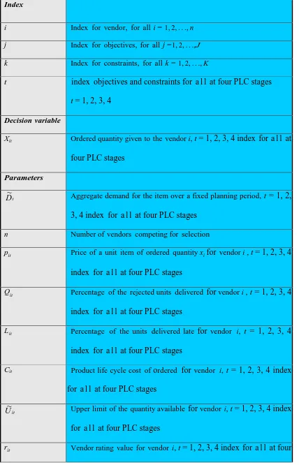
Table 1 Nomenclature [fuzzy parameters are shown with a tilde (~)]

Index

i Index for vendor, for all i = 1, 2, . . ., n

j Index for objectives, for all j =1, 2, . . .,J

k Index for constraints, for all k = 1, 2, . . ., K

t index objectives and constraints for a l l at four PLC stages t = 1, 2, 3, 4

Decision variable

Xit Orderedquantity given to the vendor i, t = 1, 2, 3, 4 index for a l l at

four PLC stages

Parameters

Dt

~ _{Aggregate demand for the item over a fixed planning period, t = 1, 2,}

3, 4 index for a l l at four PLC stages

n Number of vendors competing for selection

p_it Price of a unit item of ordered quantity xifor vendor i , t = 1, 2, 3, 4

index for a l l at four PLC stages

Q_it Percentage of the rejected units delivered for vendor i , t = 1, 2, 3, 4 index for a l l at four PLC stages

Lit Percentage of the units delivered late for vendor i, t = 1, 2, 3, 4

index for a l l at four PLC stages

Cit Product life cycle cost of ordered for vendor i, t = 1, 2, 3, 4 index

for a l l at four PLC stages

Uit

~ _{Upper limit of the quantity available for vendor i,t = 1, 2, 3, 4 index}

for a l l at four PLC stages

PLC stages

Pit The total purchasing value that a vendor can have, t = 1, 2, 3, 4

index for a l l at four PLC stages

f _it Vendor quota flexibility for vendor i, t = 1, 2, 3, 4 index for a l l at four PLC stages

Fit The value of flexibility in supply quota that a vendor should have,t =

1, 2, 3, 4 index for a l l at four PLC stages

Bit Budget constraints allocated to each vendor, t = 1, 2, 3, 4 index for

a l l at four PLC stages

Table 2 Vendor source data for the problem

Vendor No. Pi ($) Ri (%) Li (%) Ci ($) Ui (Units) r i Fi B i ($)

1 3 0.05 0.04 1.92 5,000 0.88 0.02 25,000

2 2 0.03 0.02 1.04 15,000 0.91 0.01 100,000

3 6 0.01 0.08 3.94 6,000 0.97 0.06 35,000

Table 3 Limiting values in the membership function for net cost, rejections, late deliveries, PLC cost, vendor capacities and budget information. (Data for all four stages: introduction, growth, maturity, decline)

(min.)  1 (max.)  0

Main Goals

(Gl)Net cost objective

(G2) Rejection objective

(G3) Late deliveries objective

(G4) PLC cost objective

(G5) Vendor 1

(G6) Vendor 2

(G7) Vendor 3

57,000

413

604

10,000

5,000

15,000

6,000

71,833

521

816

90,000

5,500

16,500

Budget constraints

(G8) Vendor 1

(G9) Vendor 2

(G10) Vendor 3

25,000

100,000

35,000

27,500

110,000

38,500

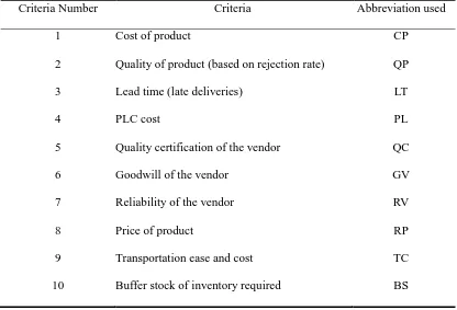
Table 4 VSPLCC criteria and abbreviations (adopted and modified from Kumar et al., 2009)

Criteria Number Criteria Abbreviation used

1 Cost of product CP

2 Quality of product (based on rejection rate) QP

3 Lead time (late deliveries) LT

4 PLC cost PL

5 Quality certification of the vendor QC

6 Goodwill of the vendor GV

7 Reliability of the vendor RV

8 Price of product RP

9 Transportation ease and cost TC

Table 5 The geometric mean matrix for the criteria of the VSPLCC problems

Criteria CP QP LT PL QC GV RV RP TC BS RW NW

CP 1 6 4 9 3 4 9 9 8 2 4.4939 0.2958

QP 0.167 1 0.500 3 0.333 0.333 2 4 5 0.250 0.8798 0.0579

LT 0.250 2 1 4 0.500 0.500 3 5 6 0.333 1.3110 0.0863

PL 0.111 0.333 0.250 1 0.200 0.500 2 3 3 0.167 0.5551 0.0365

QC 0.333 3 2 5 1 1 4 6 7 0.500 1.9608 0.1291

GV 0.250 3 2 5 1 1 4 6 7 0.500 1.9052 0.1254

RV 0.111 0.500 0.333 2 0.250 0.250 1 3 4 0.200 0.5949 0.0392

RP 0.111 0.250 0.200 0.500 0.167 0.167 0.333 1 2 0.125 0.3026 0.0199

TC 0.125 0.200 0.167 0.333 0.143 0.143 0.250 0.500 1 0.111 0.2288 0.0151

BS 0.500 4 3 6 2 2 5 8 9 1 2.9612 0.1949

Table 6 AHP method weight and supertransitive approximation with geometric mean Criteria number CriteriaAH AHP method weight

max= 10.77

Supertransitive proximation

max= 9.94

1 CP 0.2958 0.3020

2 QP 0.0579 0.0611

3 LT 0.0863 0.0810

4 PL 0.0365 0.0272

5 QC 0.1291 0.1226

6 GV 0.1254 0.1294

7 RV 0.0392 0.0376

8 RP 0.0199 0.0193

9 TC 0.0151 0.0142

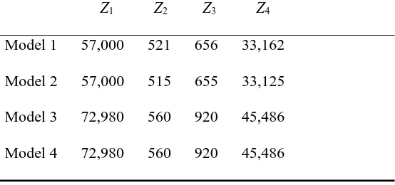
Table 7 PLCC model during the first stage (Introduction) Z1 Z2 Z3 Z4

Model 1 57,000 521 656 33,162

Model 2 57,000 515 655 33,125

Model 3 72,980 560 920 45,486

Model 4 72,980 560 920 45,486

Table 8 PLCC during the second stage (Growth)

Z1 Z2 Z3 Z4

Model 1 57,000 521 656 29,438

Model 2 57,000 515 655 29,450

Model 3 71,980 440 880 39,187

Model 4 57,000 515 655 29,450

Table 9 PLCC during the third stage (Maturity) Z1 Z2 Z3 Z4

Model 1 57,000 521 656 26,465

Model 2 57,000 515 655 26,508

Model 3 71,980 440 880 34,709

Model 4 57,000 515 655 26,507

Table 10 PLCC during the fourth stage (Decline)

Z1 Z2 Z3 Z4

Model 1 57,000 521 656 30,923

Model 2 57,000 515 655 30,880

Model 3 71,980 440 880 40,467

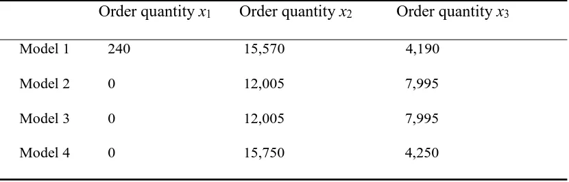
Table 11 PLCC during the first period (Introduction)

Order quantity x1 Order quantity x2 Order quantity x3

Model 1 240 5,570 4,190

Model 2 0 5,570 4,250

Model 3 5,000 8,005 6,995

Model 4 0 15,750 4,250

Table 12 PLCC during the second period (Growth)

Order quantity x1 Order quantity x2 Order quantity x3

Model 1 240 15,570 4,190

Model 2 0 12,005 7,995

Model 3 0 12,005 7,995

Model 4 0 15,750 4,250

Table 13 All of the models for order quantity of vendor x1 in the fourth PLC stages Stages of PLC Model 1 Model 2 Model 3 Model 4

Introduction 240 0 5,000 0

Growth 240 0 0 0

Maturity 240 0 0 0

Decline 240 0 0 0

Table 14 All of the models for order quantity of vendor x2 in the four PLC stages

Stages of PLC Model 1 Model 2 Model 3 Model 4

Introduction 15,570 15,570 8,005 15,570

Growth 15,570 12,005 12,005 15,750

Maturity 15,570 15,750 12,005 15,750

Table 15 All of the models for order quantity of vendor x3 in the four PLC stages Stages of PLC Model 1 Model 2 Model 3 Model 4

Introduction 4,190 4,250 6,995 4,250

Growth 4,190 7,995 7,995 4,250

Maturity 4,190 4,250 7,995 4,250