The simplification, solution and estimation of a small open DSGE model:Evidence from the UK and Canada

(1)

The Simplification, Solution and Estimation of a

Small Open DSGE Model:Evidence from the UK

and Canada

Lancaster University

LI JINYU

November 23, 2019

This dissertation is submitted for the degree of Doctor of

Philosophy

(2)

Dedication

This thesis is dedicated to my parents who encouraged me to pursue the goal of

(3)

Declaration

This thesis has not been submitted in support of an application for another degree

at this or any other university. It is the result of my own work and includes

noth-ing that is the outcome of work done in collaboration except where specifically

indicated. Many of the ideas in this thesis were the product of discussion with my

supervisor David Peel and Alina Spiru.

The thesis is being submitted in partial fulfillment of the requirements for the

degree of:. . . .PhD. . . .

I give consent for my thesis to be available for photocopying and for inter library

loan, and for the title and summary to be made avalibale to outside organisations.

Signed: LI JINYU

(4)

The Simplification, Solution and Estimation of a Small Open DSGE

Model:Evidence from the UK and Canada

Abstract

This thesis makes three main contributions to the literature on Dynamic

Stochas-tic General Equilibrium (DSGE) models. The first contribution is to bridge the

gap between a theoretical small open DSGE model provided by Gali and

Mona-celli and an empirical model developed by Lubik and Schorfheide, as no previous

studies have shown their relationship explicitly. Since all the models suffer from

the misspecification problem to some extent, the second contribution is to

ap-ply two methodologies including DSGE-VAR approach and indirect inference to

study the effect of the possibly misspecified equation of the change rate of terms

of trade. The third contribution is to search for the model with the best data

fit-ting in two stages of model comparisons. The thesis assumes that the parameters

of the simplified DSGE model are constant at the first stage, and based on the

constant parameter models with the best performance on data fitting, it assumes

a subset of the parameters including exogenous shock variances and policy

param-eters follow two independent Markov-switching Markov chains at the second stage.

The empirical results are quite different for the UK and Canada within the sample

period covering 1992: Q4 – 2008: Q4. The UK data supports that the movement

of the nominal exchange rate should not enter into the monetary policy reaction

function. Also, the data supports that it is possible for the UK to experience

the two kinds of structural changes, including the economic environment and the

(5)

Acknowledgements

It is necessary to thank many people who help me to finish the thesis. First, my

thanks go to my supervisor David Peel and Alina Spiru. Professor David suggests

me to start my research from Gali and Monacelli’s’ model and motivates me to

carry on the research of model comparisons. Alina is very patient to help me to

clarify my research questions and the relevant research methodologies.

Second, I want to appreciate Giorgio Motta and Efthymios Pavlidis. Giorgio give

me the first DSGE lectures since I joined Lancaster University since 2014, and he

also provides much additional help through my research. Efthymios used to be my

PhD director, and he always can offer me much help when something does not go

well.

I also thank Professor Xu Wenli from ANHUI University and PhD Nan Yi in

Harbin Institute of Technology in China, Professor Hirokuni Iiboshi from Tokyo

Metropolitan University in Japan. Professor Xu recommends me to use the tool

RISE to study the Markov-Switching DSGE models, and Nan Yi provides much

help when I have some coding problems with Matlab. Professor Iiboshi is so kind

that he offers me his code resources to solve a standard Markov-Switching New

Keynesian model numerically.

Lastly, I give my deepest thanks to my parents, who never get bored with me

(6)

List of Tables

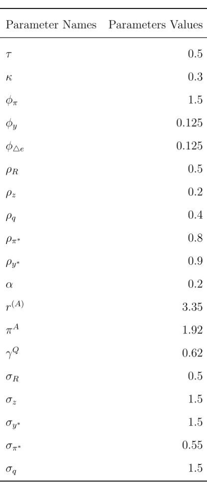
1.1 Calibration . . . 42

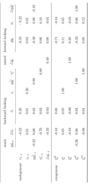
1.2 Numerical Solutions for the Calibrated Parameters . . . 46

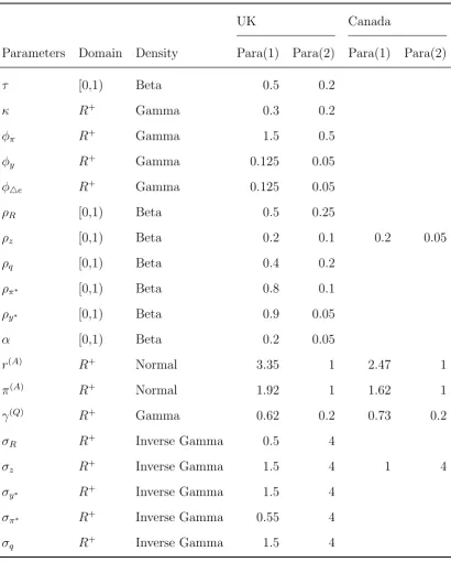
2.1 Prior Distributions for the UK and Canada . . . 66

2.2 Parameter Estimation Results for the UK and Canada . . . 71

2.3 Numerical Solutions for the UK (Benchmark Model) . . . 77

2.4 Numerical Solutions for Canada (Benchmark Model) . . . 84

2.5 The Calibration of DSGE Prior Weights λ . . . 90

2.6 Power of the Wald Test at 5% significance level . . . 94

3.1 Constant Parameter Estimation Results (Control Group) . . . 104

3.2 Constant Parameter Estimation Results (Group One) . . . 106

3.3 Numerical Solutions for the UK in the Group One . . . 110

3.4 Numerical Solutions for Canada in the Group One . . . 115

3.5 Constant Parameter Estimation Results (Group Two) . . . 118

3.6 Numerical Solutions for the UK in the Group Two . . . 122

3.7 Numerical Solutions for Canada in the Group Two . . . 127

3.8 Constant Parameter Estimation Results (Group Three) . . . 130

3.9 Numerical Solutions for the UK in the Group Three . . . 134

3.10 Numerical Solutions for Canada in the Group Three . . . 139

3.11 Numerical Results of the Posterior Odds Ratio . . . 143

3.12 The Rank of the Data Fitting Performance of Each Group . . . 143

4.1 Parameter Estimation Results of the Benchmark Models . . . 152

(10)

4.3 Model One with Markov-Switching Variances(UK) . . . 156

4.4 The Numerical Solution to Regime 1 of the Model One for the UK . 160

4.5 The Numerical Solution to Regime 2 of the Model One for the UK . 161

4.6 Variance Decomposition of the Model One for the UK . . . 165

4.7 Model Two with Markov-Switching Policy Parameters(UK) . . . 167

4.8 The Numerical Solution to Regime 1 of the Model Two for the UK 171

4.9 The Numerical Solution to Regime 2 of the Model Two for the UK 172

4.10 Variance decomposition of the Model Two for the UK . . . 176

4.11 Model Three with 2 Markov Chains(UK) . . . 179

4.12 The Numerical Solution to Regime 1 of the Model Three for the UK 186

4.16 Variance Decomposition of the Model Three for the UK . . . 194

4.17 Log Marginal Data Densities and Ranks of the Models for the UK . 198

4.18 Prior Distributions of the Structural Parameters for Canada . . . . 203

4.19 Model One with Markov-Switching Variances(Canada) . . . 205

4.20 The Numerical Solution to Regime 1 of the Model One for Canada 209

4.21 The Numerical Solution to regime 2 of the Model One for Canada . 210

4.22 Variance Decomposition of the Model One for Canada . . . 214

4.23 Model Two with Markov-Switching Policy Parameters(Canada) . . 216

4.24 The Numerical Solution to Regime 1 of the Model Two for Canada 220

4.25 The Numerical Solution to Regime 2 of the Model Two for Canada 221

4.26 Variance Decomposition of the Model Two for Canada . . . 225

(11)

(12)

List of Figures

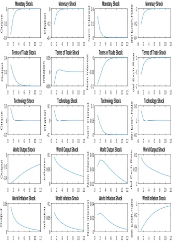
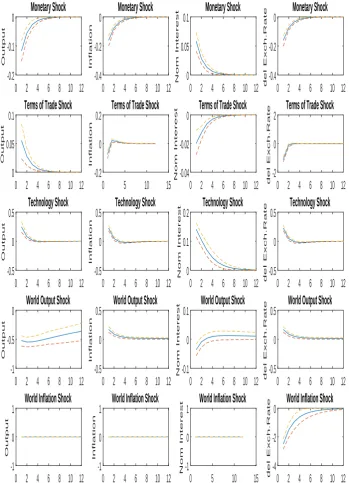
1.1 Impulse response functions for the Calibrated parameters . . . 47

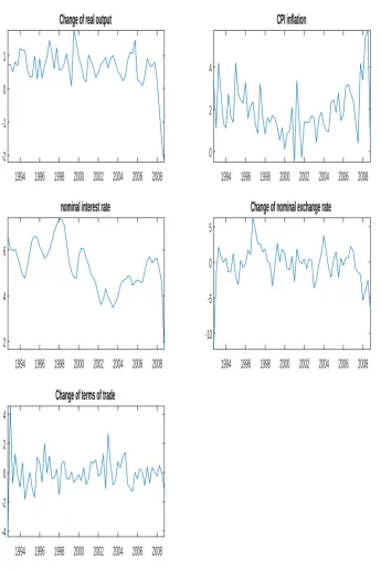
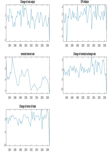
2.1 Data of UK . . . 55

2.2 Data of Canada . . . 58

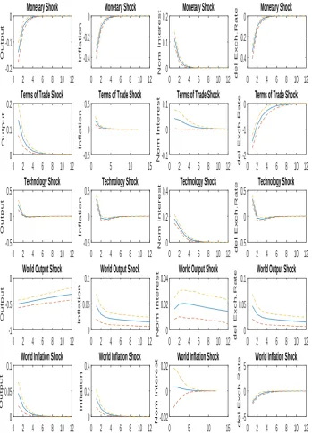
2.3 Impulse response functions for the benchmark model in the UK . . 78

2.4 Impulse response functions for the benchmark model in Canada . . 85

2.5 Calibrations of DSGE Prior Weights . . . 91

3.1 Impulse response functions for Group One in the UK . . . 111

3.2 Impulse response functions for Group One in Canada . . . 116

3.3 Impulse response functions for Group Two in the UK . . . 123

3.4 Impulse response functions for Group Two in Canada . . . 128

3.5 Impulse response functions for Group Three in the UK . . . 135

3.6 Impulse response functions for Group Three in Canada . . . 140

4.1 Impulse responses,UK(Markov-switching Model One) . . . 162

4.2 Impulse responses,UK(Markov-switching Model Two) . . . 173

(13)

4.8 Impulse responses,Canada(Model One) . . . 211

4.9 Impulse responses,Canada(Model Two) . . . 222

4.10 Impulse responses,Canada(Switching Variances of Model Three) . . 239

4.11 Impulse responses,Canada(Switching Taylor Rules of Model Three . 240

4.12 Smoothed probability of high volatility from model one . . . 247

4.13 Smoothed probability of strict inflation from model two . . . 248

(14)

General Introduction

The main objective of the thesis is to answer the question that how to improve the

data fitting for a given DSGE model based on different specifications of monetary

policy function and some subsets of parameter space following Markov-Switching

chains. The thesis will prefer the UK and Canada as two sample countries within

the sample period 1992:Q4-2008:Q4. There are mainly three reasons motivating

the preference. First, the DSGE model adopted by the thesis is appropriate for

small open economies, which includes features that the UK and Canada hold to

some extent. Second, the UK and Canada share something in common within the

chosen sample period. They both announce that they adopt inflation targeting

monetary policy after the early 1990s. This thesis does not consider the periods of

the zero lower bound after 2008 when the conventional monetary policy does not

work. Third, the UK and Canadian monetary policy also exhibit some different

features within the chosen sample period. There is a debate about whether the

movement of the nominal exchange rate should enter into the design of the

mon-etary policy. Overall, the thesis will study the two sample countries within the

sample period at the same time and exhibit their similar and different features,

(15)

makers about the impact and feedback of their conduct policy in an economy with

assumptions of the real business cycle or New Keynesian nominal rigidity, which

plays an increasingly key role in the modern macroeconomic analysis. Ramsey

(1927[73],1928[74]) initially mature the framework of this approach. Subsequently,

Cass (1965[13]) and Koopmans(1965[54]) carry on developing this methodology.

The Lucas critique (Lucas, 1976[61]) and the urgent need to set up micro-founded

macroeconomic models lead to a revolution in macroeconomics in the 1980s. It is

Kydland and Prescott (1982[55]) who set up the vital work in modern

macroeco-nomic analysis, which is famous for the starting point of the Real Business Cycle

(RBC) theory. In the combination between the developed economic theory and the

major events in the 20st, the size of DSGE model becomes larger and the

struc-ture of it becomes more complicated, because DSGE models gradually

incorpo-rate a large number of New Keynesian features(Rotemberg,1982[76];Blanchard and

Kiyotaki,1987[9]; Rotemberg and Woodford,1997[77]; Woodford,2011[93];Smet and

Wouters, 2003[82],2007[83]). At the meantime, instead of studying the policy and

the economy isolated from the world, Some individuals including Clarida,Gali and

Gertler (2001[20];2002[21]),Gertler, Gilchrist and Natalucci(2007[38])and

Mona-celli (2005[66]) start extending the DSGE framework to the context of an open

economy in the presence of the trade sector and the currency values in their

mod-els. Gali and Monacelli (2005[37]) develop a critical theoretical DSGE model which

describe a small open economy which is allowed to trade with the rest of the world

and hardly impose a significant impact on the global economy. This model with

calibrated parameters can be regarded as the seminal one to guide the policy

mak-ers to design the optimal monetary policies. Unexpectedly, as pointed by Diebold

(1998[27]), the large scale and the complicated structure of the models may

pre-vent us from measuring the estimates of parameters efficiently and consistently.

Some individuals then simplify Gali and Monacelli’s framework, and among them,

Lubik and Schorfheide (2007[60])’s simplification is applied for practical purpose

in terms of constant parameter model (Zheng and Guo,2013[94].) and

(16)

literature, including Lubik and Schorfheide, clearly explain the relationship

be-tween the theoretical model and the empirical one in terms of the model variables

and the parameters. To use their model directly may confuse others because there

is not a clear transition from the micro-foundations to the simplified model.

Ac-cordingly, the lack of transparency motivates the thesis to set up a bridge between

the theoretical model and the simplified one. Chapter 1 of the thesis replicates the

derivation process of the empirical model and stands out the meaning of the

vari-ables and parameters in the simplified model, thereby identifying whether there are

(17)

The Solutions to the DSGE Models

The solution to a DSGE model is approximately a VAR model with restricted

co-efficients deriving from the structural parameters. Blanchard and Kahn (1980[8])

develop a solution method which provides an important condition for the existence

and uniqueness of the solutions to the system. That is, the number of explosive

eigenvalues should be exactly equal to the number of jump variables with the

ex-pectation operators. Sims (2002[80]) proposes a solution method, which is a bit

different from Blanchard and Kahn’s work. Although they still decouple the

sys-tem of models into explosive and nonexplosive portions, the expected errors instead

of the expectation operators appear in the system. Besides, the technique of QZ or

Schur decomposition is applied in their methodology to overcome the singularity

of the matrix coefficients. Klein (2000[51]) develops a method which is a hybrid

of those of Blanchard and Kahn (1980[8]) and Sims (2001[80]). Like Blanchard

and Kahn’s method, he distinguishes the predetermined and jump variables of the

system. Also, the QZ technique is applied to solve the system in the absence of

expectation errors. Furthermore, Uhlig (1995[89]) develops an undetermined

coef-ficient approach, which is very different from the other methodologies. Rather than

focusing on solving the system with different portions, he tries to uncover the

rela-tionships among the parameters and solve them once for all. Moreover, Svensson

and Williams (2005[85]), Farmer et al(2011[32]), Cho (2014[17]) introduce Markov

switching to the parameters of the system. They solve the Markov-Switching

DSGE model through solving a constant parameters model with the structural

parameters and the transition probabilities. They have proved that their

solu-tions are unique and stable. In a word, Blanchard and Kahn’s approach is the

fundamental one for this thesis to solve the simplified DSGE model, which also

incorporates the techniques of QZ decomposition as does in Sims and Klein’s work.

It is often difficult to solve the model by hand when the number of the

equa-tions and variables are many even for an already simplified system. Thus, it is

(18)

packaged in some powerful software such like Matlab(Judd, 1998[46]; Miranda

and Fackler, 2004[65]; Woodford and Philips, 2011[92]; Brandimarte,2013[10])

and a newly invented software Julia (Caraiani,2018[12]). In this thesis, Dynare

(Adjemian,2011[1]) is the primary tool to solve the constant parameter DSGE

models and Rise (Maih,2015[62])) is a very efficient tool to solve the

(19)

The Bayesian Estimation of DSGE Models

The thesis will estimate the DSGE models with the Bayesian methodology and

evaluate their performances of data fitting with the posterior likelihood ratio test.

The combination between a prior probability distribution and the maximum

like-lihood function of the data in the Bayesian approach can construct a posterior

probability distribution which provides a full statistical characterisation of the

observed data. Geweke (1999[39]) and Robert and Casella (2013[75]) provide a

numerical approach to calculate the integration of the posterior probability

den-sities in the Bayesian framework. Bauwens et al. (2000[5]) offer an application of

Bayesian methods to study a wide range of dynamic reduced-form models.

More-over, Koop (2003[53]) writes a textbook which incorporates a general overview of

Bayesian statistical methods with further details regarding computational issues.

It is not very common to estimate DSGE models with Bayesian methodology

un-til Smet and Wouters (2003[82], 2007[83]) use this approach to estimate a closed

DSGE model for the US economy with data covering the period 1966: Q1-2004:

Q4. After that, Adolfson et al. (2007[2]) extend and estimate the model

de-veloped by Christiano (2005[18]) for the Eurozone with data covering the period

1970: Q1-2002: Q4. An and Schorfheide (2007[3]) estimate the DSGE model

developed by Woodford (2011[93]) with artificial data and evaluate the model

with posterior odds ratio and DSGE-VAR approach. In addition to the

devel-oped countries, Gabriel et al. (2010[33]) estimate a DSGE model in the

pres-ence of financial frictions with Indian data covering period 1980: Q1-2006: Q4.

Zheng and Guo (2013[94]) estimate the DSGE model developed by Lubik and

Schorfheide(2007[60]) with China data covering the period 1992: Q1-2011: Q4.

There are also some useful textbooks regarding the Bayesian estimation of DSGE

models (Dejong and Dave,2011[23]; Hashimzade and Thornton,2013[41]; Herbst

and Schorfheide, 2015[42]). It is exceedingly beneficial to use such textbooks to

(20)

Lubik and Schorfheide (2007[60]) offer the primary motivation for my research.

They estimate a small open DSGE model, which is a simplified version of Gali

and Monacelli’s model, with the data of Canada, Britain, New Zealand and

Aus-tralia covering the period 1983: Q1-2002: Q4. They consider two versions of the

model with different specification of Taylor principle rules and conclude that it

offers the best data fitting for the UK and Canada when it considers the

move-ment of the nominal exchange rate in the policy reaction function. However, the

empirical results for the UK are not approved by the Bank of England in their

release. The sample period they choose includes at least one structural change

when the UK is no longer a member of the Exchange Rate Mechanism (ERM)

since 1992. The thesis will adopt a new sample size of the UK and Canada

cov-ering the period 1992: Q4-2008: Q4, which excludes the period when the UK is

a member of ERM and extends the period until the nominal interest rates

ex-perience zero lower bound in the recent financial crisis. Chapter 2 will estimate

the original Lubik and Schorfheide’s model with the new sample size and reserve

the results as a control group in the next chapter. Moreover, it will borrow two

methodologies developed from Le et al. (2013[56]) and Del Nergo et al. (2007[26])

to identify the misspecification problems of the small open DSGE model

consid-ering whether there is a unit process of the rate change of the terms of trade or not.

Taylor rule policy reaction function (1993[86]) is the equation with different

specifi-cations in the estimation. Taylor originally includes the inflation rate and the

out-put gap in the policy reaction function. Gradually, its structure has been changed

a lot in examining the coefficients of monetary policy reaction functions in

(21)

type of monetary policy with the US data covering the period 1982: Q1-2003: Q1.

This type of rule is also applied by Smet and Wouter (2007) in their DSGE model.

Overwhelmingly, the policy reaction function incorporates four kinds of

specifica-tions based on a combination between the existence of the nominal exchange rate

depreciation and the rate change of output. Among them, the original one in Lubik

and Schorfheide’s model is regarded as the control group while others comprise of

the treatment groups. Chapter 3 of the thesis compares the four groups and finds

the model with the best data fitting in using the Bayesian likelihood approach.

The model with the best fitting performance will be the benchmark model for the

next chapter.

Some economies inevitably have experienced structural changes in the past decades.

For instance, Nelson(2003[67]) offers guidance of the regime changes of UK

mon-etary policy covering the period 1972-1997, from the period of floating exchange

rate to the period of independence of the Bank of England. VARs model is

a convenient methodology to study the regime shifts (Catelnuovo and Surico

,2005[14];Benati,2009[6]). Since Davig and Leeper (2006[22]) and Farmer et al.

(2011[32]) can provide a unique solution to the Markov-Switching rational

ex-pectation models, it motivates individuals to identify the regime shifts in

differ-ent countries based on diversified versions of DSGE models. Benati and Surico

(2009[6]) estimate a Markov-Switching New Keynesian model with US data

cov-ering the period of the Great Moderation. Liu and Mumtaz (2011[57]) initially

examine the UK data with a small open Markov-Switching DSGE model developed

from Justiniano and Preston (2010[48]) covering 1970: Q1-2009: Q1. Chen and

MacDonald(2012[16]) estimate a small open DSGE model developed by Lubki and

Schorfheid (2007[60]) covering the period 1975:Q1-2010:Q2. Here is one thing to

mention, the models developed from Justiniano and Preston (2010[48]) and Lubki

and Schorfheid (2007[60]) are both the simplified version of Gali and Monacelli

(2005[37])’s framework. Chapter 4 will introduce two similar kinds of Markov

(22)

DSGE model which offer the best data fitting in the previous chapter. Chapter 4

tries to find the Markov-switching DSGE model with the best data fitting, and it

mainly has three aspects different from the previous literature. First, the chosen

sample size is shorter and covers the period 1992: Q4-2008: Q4. The chosen period

excludes the potential impacts of the fixed exchange rate regime and the zero lower

bound on the monetary policy reaction function. Second, chapter 4 borrows the

specification of the monetary policy reaction function offering the best data fitting

for each country from the constant parameter estimation in chapter 3. At last,

chapter 4 only considers two kinds of structural changes, including the variance of

(23)

The Structure of the Thesis

There are five chapters in this thesis. Chapter 1 will derive the core parts of

the theoretical small open DSGE model proposed by Gali and Monacelli. It then

uncovers the simplification process from the theoretical model to the empirical one

provided by Lubik and Schorfheide. At the end of chapter one, it will exhibit a

classical method combined with Dynare to solve the model numerically. Chapter

2 will describe the data sample and then introduces the Bayesian methodology

to estimate the model for the UK and Canada separately. Moreover, it provides

two alternative methodologies linking VARs to DSGE models, thereby checking

the model identification regarding the equation of the change rate of the terms of

trade. Chapter 3 will regard the empirical results from chapter 2 as the control

group and have another three treatment groups based on different specifications of

the monetary policy reaction function. It will search for the model with the best

performance of data fitting for each of the two countries. Chapter 4 will regard

the model with the best performance of data fitting in chapter 3 as the benchmark

model and introduce two types of Markov-Switching parameters in the small open

DSGE model. It will carry on searching for the model with the best performance

of data fitting within the same sample period and tries to answer whether there is a

significant improvement of data fitting between the constant parameter model and

the Markov-Switching DSGE model. Chapter 5 summarises the main findings of

the thesis and offers some implications of the current research with further possible

(24)

Chapter 1 The Simplification and Solution

of the Model

1.1 Introduction

The thesis will borrow the small open DSGE model from Lubik and Schorfheide

(2007)[60]’s research. This log-linear model is a simplified version of the model

developed by Gali and Monacelli (2005)[37]. There are two economies in this

model. One is the home country, and the other one is the rest of the world. The

DSGE model comprises of a forward-looking IS equation, a forward-looking Philip

curve, an exchange rate equation derived based on the law of one price and a

Taylor type monetary policy rule and four exogenous stationary processes. In the

log-linear model, the log differences of economic variables express the percentage

deviations of such variables concerning their stable states. There are two sections

in this chapter. The first section will show the derivation process of the

(25)

1.2 A Small Open DSGE Model

This section will present the main components of a small open DSGE model derived

by Gali and Monacelli(2005 [37]). After that, it will uncover the process of how

Lubik and Schorfheide (2007[60]) simplify the model from the previous work. The

simplified version of the model has been used in the empirical research to study the

behaviour of central banks in different countries(Zheng and Guo (2013[94]), Chen

and Macdonald(2012[16])). However, few of them, even Lubik and Schorfheide

themselves, has explicitly revealed the process to generate the simplified model

from Gali and Monacelli’s work. By uncovering the connections between the two

versions of models, this section is helpful to understand the assumptions and the

limitations of the model better.

1.2.1 Types of Model Variables

It is essential to introduce the types of model variables adopted in the DSGE model

in this section. For instance, ifMt is an arbitrary type of economic variable, then

mt is the log value of the economic variable: mt=logMt. ˜mt is the log difference

of the economic variable: m˜t = mt −m = logMt−logM = Mt_M−M,where M is

the steady state of the economic variable. Lubik and Schorfheide opt for ˜mt in

their DSGE model and the steady state ˜mis zero, which implies that the economic variablesMt will converge to their stationary statesM in the equilibrium level.

1.2.2 Gali and Monacelli’s framework

Gali and Monacelli’s framework incorporates about eight segments which are

rele-vant to the following simplifying process. The first segment discusses the

intertem-poral optimal condition of the household. The second one brings in the definition

of terms of trade given the steady state of the purchasing power parity. The third

one assumes there is an uncovered interest parity between any two countries in

the bond market. The fourth one shows a retailer firm in the market of perfect

(26)

mo-nopolistic competition. The sixth one exhibits the optimal pricing strategy of the

wholesale firms when the price is sticky according to the Calvo rule (1983[11]).

The seventh segment displays the relationship between the consumption and

out-put in the given small open economy. The final one obtains the potential outout-put

and natural rate of the interest rate. The equations and the dependent

parame-ters generated from such eight segments will play critical roles in the simplifying

process.

Households

The representative household optimises the following utility function:

E0

∞

X

t=0

βt

C_t1−σ 1−σ −

N_t1+ϕ 1 +ϕ

, (1.1)

where Nt is hours of labour, Ct is a composite consumption index, β is the

in-tertemporal discount factor, σ is the relative risk aversion coefficient and ϕ is the marginal disutility with respect to labour supply. In addition, The composite

consumption indexCt can be defined as:

Ct=

h

(1−α)1/η(CH,t)(

η−1

η )+α1/η(C

F,t)(

η−1

η )

i_η₋η₁

, (1.2)

where CH,t is an index of consumption of domestic produced goods, CF,t is an

index of imported goods, η measures the elasticity of substitution between such two kinds of goods, andα is an index of openness. The equation defining CH,t is:

CH,t =

Z 1

0

CH,t(j)

ξ ε−1dj

ξ−ξ1

, (1.3)

whereCH,t(j) represents the consumption of home product of goodj at timet, and

(27)

in the world. Moreover, Ci,t consists of a continuum of differentiated goods in the

unit interval:

Ci,t =

Z 1

0

Ci,t(j)

ξ ε−1dj

ξ ξ−1

, (1.5)

where Ci,t(j) represents the consumption of product of good j imported from a

foreign countryi at timet.

It assumes that the total consumption from goods market and bond market cannot

exceed the revenue in each period. Thus, the household’s period budget can be

written as

Z 1

0

PH,t(j)CH,t(j)dj+

Z 1

0

Z 1

0

Pi,t(j)Ci,t(j)djdi+Et[Qt,t+1Dt+1]≤Dt+WtNt+Tt,

(1.6)

where PH,t(j) is the price of home product of good j, Pi,t(j) is the price of good

j imported from country i. Qt,t+1 is the stochastic discount factor for the

nomi-nal payoffs Dt+1 in the period t+ 1 of the bond held at the end of period t. Wt

is the nominal wage andTtis the lump sum transfers (positive) or taxes (negative).

The next task is to take i,j,H and F off from the budget constraint. First, max-imise equation (1.3) given the constraint:

Z 1

0

PH,t(j)CH,t(j)dj =PH,tCH,t. (1.7)

The maximisation procedures arrive at the demand function of the domestic good

j.

CH,t(j) =

PH,t(j)

PH,t

−ξ

CH,t. (1.8)

Substitute the above equation in the equation (1.7) yields the domestic price index:

PH,t = (

Z 1

0

PH,t(j)1−ξdj)

1

1−ξ. (1.9) Second, maximise equation (1.5) given the constraint:

Z 1

0

(28)

The demand function of the imported good j from a foreign countryi is

Ci,t(j) =

Pi,t(j)

Pi,t

−ξ

Ci,t. (1.11)

Likewise, the price index(expressed in home currency) for imported goods from

countryi can be written in the following way:

Pi,t = (

Z 1

0

Pi,t(j)1−ξdj)

1

1−ξ. (1.12) By far, it is ready to take j away from the period budget constraint (1.6). Third, maximise equation (1.4) given the constraint

Z 1

0

Pi,tCi,tdi=PF,tCF,t. (1.13)

The demand function of the imported good for a given countryi is

Ci,t =

Pi,t

PF,t

−γ

CF,t. (1.14)

The price index (expressed in home currency) for imported goods is

PF,t= (

Z 1

0

P_i,t1−γdi)1−1γ_. _(1.15) Now it is ready to take i away from the period budget constraint (1.6). Fi-nally,maximise equation (1.2) given the constraint:

PH,tCH,t+PF,tCF,t=PtCt. (1.16)

The demand function of the domestic goodCH,t is given by

CH,t = (1−α)

PH,t

Pt

−η

Ct. (1.17)

The demand function of the imported good CF,t is given by

CF,t=α

PF,t

P −η

(29)

Turning back to the maximisation of the representative household’s utility (1.1)

given the above budget constraint leads to the intertemporal optimal condition.

βRtEt

(Ct+1 Ct

)−σ( Pt Pt+1

)

= 1. (1.21)

where Rt = _E_t_Q1_t,t₊₁ is the gross return on a risk free one period discount bond

paying off one unit of home currency at time t + 1.Rewrite the intertemporal condition in the log-linear form:

˜

ct =Etct˜+1−

1

σ(rt−Etπt+1−ρ), (1.22)

wherert=Rt−1 is the net interest rate, πt=log(Pt)−log(Pt−1) is CPI inflation,

and ρ= _β1 −1 is the time discount rate.

The derivation process of the household section is the very key component in

the framework of a DSGE model. In addition to Gali and Monacelli (2005[37]),

the famous book written by Gali(2015[35]) and Walsh (2017[91]) offer a very

speci-fied explanation and illustration of the optimal conditions of households in a small

open economy. More specifically,the latter one also includes a two-country model

developed by Obstfeld and Rogoff (1995[68];1996[69]). The two-country model is

useful when someone is interested in examining the impact of national

develop-ment on the international economy. The thesis is consistent with Gali(2015[35])’s

framework, which assumes the domestic economy is tiny and have little impacts

(30)

Purchasing Power Parity and Law of One Price

Gali and Monacelli (2005[37]) define the effective terms of tradeStas the following

equation:

St=

PF,t

PH,t

=

Z 1

0

S_i,t1−γdi 1−1γ

, (1.23)

whereSi,t =

Pi,t

PH,t is the bilateral terms of trade between the home economy and a foreign country i. In addition, the price of country i’s goods Pi,t is expressed in

the domestic currency. Given the assumptions that the steady state satisfying the

purchasing power parityS = 1 and the elasticity of substitution between different countriesγ = 1, rewrite the formula above in the log-linear from:

˜

st = (pF,t−pF)−(pH,t−pH) = pF,t−pH,t =

Z 1

0

˜

si,tdi. (1.24)

Analogically, under the assumption of purchasing power parity and the elasticity

of substitution between home product and imported goodsη= 1, rewrite the CPI price formula (1.19) in the log-linear expression:

pt= (1−α)pH,t+αpF,t=pH,t+αs˜t. (1.25)

Take one period backward of the above equation and subtract it from the above

equation yield the following relationship between the CPI inflation and domestic

inflation.

πt =πH,t+α4s˜t, (1.26)

where the domestic inflation πH,t = pH,t−pH,t−1 is defined as the rate of change

in the index of domestic goods prices.

(31)

rewritten as the following equation:

Pi,t =εi,tPi,ti =εi,t(

Z 1

0

P_i,ti (j)1−ξdj)1−1ξ (1.28) Substitute the above equation in the equation (1.15) and rewrite PF,t in the

fol-lowing equation:

PF,t=

" Z 1

0

εi,t(

Z 1

0

P_i,ti (j)1−ξdj)1−1ξ

1−γ di

#₁₋1_γ

. (1.29)

Rewrite the above equation in the log-linear form under the assumptions γ = 1 yields the equation below:

pF,t=

Z 1

0

(ei,t+pii,t)di =et+p∗t, (1.30)

where et =

R1

0 ei,tdi is the log nominal effective exchange rate, p

i

i,t =

R1 0 p

i

i,t(j)dj

is the log domestic price index for country i expressed in its own currency, and p∗_t = R1

0 p

i

i,tdi is the log world price index. Combining this formula with the

equation (1.24), the log difference of terms of trade is rewritten as the following

equation:

˜

st= ˜et+p∗t −pH,t. (1.31)

Take one period backward of the above equation and subtract it from the above

equation generates an important relationship between CPI inflation and the rate

change of nominal exchange rate in the equation below:

πt =πt∗+4e˜t−(1−α)4s˜t. (1.32)

The definition of terms of trade in Gali and Monacelli (2005[37])’s framework

is a bit different from the practical side. Chamberlin and Yueh (2006[15]) define

the terms of trade as the ratio of export to import prices, which is just the

op-posite to the definition of Gali and Monacelli (2005[37]). Generally, an exchange

rate depreciation will increase the import price and weaken the terms of trade.

(32)

sector. From the viewpoints of the import sector, the weakened terms of trade

will deteriorate the trade balance if the country does not expand the quantity of

its export. The exchange rate depreciation 4e˜t and the change rate of the terms

of trade 4s˜t should move in the opposite direction, and the simplified model will

(33)

Uncover Interest Parity and Terms of Trade

The intertemporal optimal condition for the representative household in any other

country i is written in the following equation:

βEt

(C

i

t+1

Ci t

)−σ( P

i t

Pi

t+1

)

=Qi_t,t₊₁. (1.33)

Under the assumption of law of one price and complete security markets, there are

no arbitrage opportunities in the bond market:

Qt,t+1 =Qit,t+1

εi_t εi

t+1

, (1.34)

where it implies a potential investor is able to buy the domestic bonds and the

foreign bonds at the same discounted current price expressed in the same currency.

The combination between equation (1.33) and (1.34) arrives at an uncovered

in-terest rate parity:

Rt =Rit

εi

t+1

εi t

= 1 εi t

Ri_tεi_t₊₁, (1.35)

where it implies the profit of one unit of the domestic currency invested in the

domestic bond market is same as the profit of one unit of the domestic currency

invested in the foreign bond market. Ri_t = _Qi1

t,t+1 is the foreign gross return of

one period bond and the dimension ofεi

t is

f oreigncurrency

homecurrency . Combining the equation (1.33) with equation (1.21), it yields the equation below:

Ct+1

Ct

= (

Pi

tεit

Pt

Pi

t+1εit+1

Pt+1

)−σC

i

t+1

Ci t

= ( Qi,t Qi,t+1

)−σC

i

t+1

Ci t

, (1.36)

whereQi,t =

Pi

tεit

Pt is defined as the bilateral real exchange rate for the currency in the country i. It is important to extract an important relationship between the domestic and home consumption from the above equation:

Ct=vCtiQ

1

σ

i,t, (1.37)

where v is a arbitrary constant and can be canceled off when log-linearize the

above equation around the steady stateC =Ci =C∗ under the assumption of the purchasing power parity Qi =Si = 1:

˜

ct= ˜c∗t +

1

(34)

wherec∗_t =R₀1ci_tdi is the index of world consumption andqt=

R1

0 qi,tdi=

R1

0(ei,t+

pi

t −pt) is the log effective real exchange rate. Combining equation (1.25) and

(1.31),the log difference of the real effective exchange rate is expressed by:

˜

qt = ˜et+p∗t −pt= ˜st+pH,t−pt = (1−α) ˜st. (1.39)

Substitute the real exchange rate in the equation (1.38), it yields a relationship

between the home consumption and the world consumption:

˜

ct = ˜c∗t + (

1−α

σ ) ˜st. (1.40)

In addition, log-linearize the equation (1.35) will yield a relationship between the

home net interest rate and the world net interest rate r∗_t:

rt−r∗t =Et4et˜+1. (1.41)

Combining the above equation with the equation (1.32) yields the relationship

between the interest rate and terms of trade:

˜

st= (r∗t −π

∗

t+1) + (rt−EtπH,t+1) + ˜st+1. (1.42)

Uncovered interest rate parity assumes that the bond investors will hold the bond

with the highest expected return. However, the assumption of the uncovered

in-terest rate parity is too strong for two reasons (Blanchard,2013[7]). On the one

hand, it ignores the transaction cost. For instance, entering in and exists from

the UK bond market requires three contracts with different transaction costs. On

(35)

Retailers(Final Goods Firm)

The optimisation problems are a bit complicated in the home production sector,

which require the inclusion of two sections: firms called retailers which produce

the final goods in the market of perfect competition and firms called wholesalers

which produce the intermediate goods in the market of monopolistic competition.

The wholesale firms will produce many infinitely differentiate intermediate goods

and sell them to the retailer firms with a flexible or sticky price. The retailer firms

then aggregate the intermediate goods into the same type of final goods and then

sell them with perfect competition.

The objective of the retailer is to maximise the profit in the below equation:

PH,tYt−

Z 1

0

PH,t(j)Yt(j)dj, (1.43)

with the constraint below implying that the elasticity of substitution of the many

infinitely intermediate goods is ξ:

Yt=

Z 1

0

Yt(j)

ξ−1

ξ

ξ ξ−1

. (1.44)

Accordingly, the optimisation procedures arrive at the demand function for the

wholesale good j:

Yt(j) =

PH,t(j)

PH,t

−ξ

Yt. (1.45)

Substitute the above equation and the equation (1.9) in equation (1.43), the

max-imum profit of the retailer firms is zero, which proves that there is perfect

(36)

Wholesale Firms with flexible prices strategy

Given the flexible price strategy, the objective of the wholesale firms is to maximize

the profit:

PH,t(j)Yt(j)−(1−τ1)WtNt(j) (1.46)

whereτ1 is the subsidy of employment. The objective is constrained by the

equa-tion (1.45) and the producequa-tion funcequa-tion defined as the below equaequa-tion:

Yt(j) =AtNt(j). (1.47)

The optimal price of wholesale goodj is written in the following equation:

PH,t(j) =

ξ

ξ−1M C

n

t, (1.48)

whereM C_tn= (1−τ1)W_A_tt is the nominal marginal cost. In addition, the marginal

cost is independent of j and identical for all wholesale firms. Rewrite the real

marginal cost M Ct =

M Cn

t

PH,t in the log-linear form:

mct =log(1−τ1) +wt−pH,t−at. (1.49)

(37)

Wholesale Firms with sticky prices strategy

Calvo (1983[11]) assumes the wholesale firms has a θ probability of keeping the price of its good fixed in the following periods and a 1−θ probability of optimally redefining its price. The objective of the wholesale firm to maximize the profit is

defined in the below equation:

∞

X

k=0

θkEt[Qt,t+k(Yt+k(PH,t∗ −M C n

t+k))], (1.50)

subjecting to the constraint obtained from equation (1.45):

Yt+k(j) = (

P_H,t∗ PH,t+k

)−εYt+k (1.51)

The discount factor Qt,t+k = βk(

Ct+k

Ct )

−σ₍ Pt

Pt+k) is derived from the optimal in-tertemporal condition (1.21). Under the assumptions σ = 1,η = 1 and γ = 1, it arrives at the optimal redefining priceP_H,t∗ :

P_H,t∗ = ξ

ξ−1

X1,t

X2,t

, (1.52)

where X1,t = M Ct + θβEtX1,t+1 and X2,t = PH,t−1 +θβEtX2,t+1. The optimal

resetting price is identical for all the wholesale firms. In addition, the above

equation can be represented by the domestic inflation instead of the domestic

price index:

P_H,t∗ PH,t−1

= 1 +π_H,t∗ = ξ

ξ−1

1 PH,t−1

X1,t

X2,t

= ξ

ξ−1(1 +πH,t) X1,t

X₂∗_,t, (1.53) whereX₂∗_,t= 1+βθ(1+πH,t+1)−1EtX2,t+1. Log-linearize the equation (1.53) around

the zero steady inflation rate yields:

π_H,t∗ =πH,t+ ˜x1,t−x˜∗2,t, (1.54)

where ˜x1,t = (1−θβ) ˜mct+θβEtx1˜,t+1 and ˜x∗2,t =−θβEtπH,t+1+θβEtx∗2˜,t+1. Also,

˜

mct = mct−mc is the log difference of the real marginal cost with respect to its

stationary state. Given the price stickness, the domestic price index function (1.9)

can be rewritten as follows:

P_H,t1−ξ =

Z θ

0

P_H,t1−ξ₋₁(j)dj+

Z 1

θ

(38)

The above equation can be rewritten in terms of the inflation by dividing P_t1₋−₁ξ from both sides:

(1 +πH,t)1−ξ =θ+ (1−θ)(1 +π∗H,t)

1−ξ _(1.56)

Log-linearize the function above yields the relationship between the optimal

infla-tion and the domestic inflainfla-tion:

πH,t = (1−θ)πH,t∗ (1.57)

Substitute the above equation in the equation (1.54) yields the domestic Philips

curve:

πH,t=βEtπH,t+1+κmc˜t, (1.58)

whereκ= (1−θ)(1_θ−θβ).

Monopolistic competition and the sticky prices are two central assumptions for

the supply side in the DSGE model considering the features of the New

Keyne-sian. The prices of goods are normally higher than the marginal cost, which

inval-idates the assumption of the perfect competition in the real business cycle model.

For instance, Hall(1998[40]) finds evidence of a higher price than the marginal

cost in the US economy. Dixit and Stiglitz(1997[28]) mathematically approximate

the central idea of the imperfect competition, and after that, most of the DSGE

models borrow their ideas to assume there is a continues of differentiated goods

locating in the interval from zero to one. More specifically, Torres(2015[88]) offers

an excellent and fundamental book to cover the final goods production sector

(re-tailers) in the perfect competition market and the production of the intermediate

goods sector (wholesale firms) in the monopolistic competition market. The price

(39)

Consumption and Output

The equilibrium in the goods market for the small open economy requires:

Yt(j) = CH,t(j) +

Z 1

0

C_H,ti (j)di, (1.59)

whereC_H,ti (j) represents foreign country i’s consumption for the good j produced in the home country. The simplification of the above equation needs several steps.

First, rewrite CH,t(j) in the from of Ct through the equations (1.8) and (1.17):

CH,t(j) = (

PH,t(j)

PH,t

)−ξCH,t = (

PH,t(j)

PH,t

)−ξ(1−α)(PH,t Pt

)−ηCt. (1.60)

Second, rewriteC_H,ti (j) in the form of C_H,ti through equation(1.8) :

C_H,ti (j) = (PH,t(j) PH,t

)−ξC_H,ti , (1.61)

where it implies the foreign country i prefers to consume good j from the home economy given the price of it PH,t(j) in relation to the whole price index PH,t.

Next, rewrite Ci

H,t in the form of CF,ti through equation (1.14):

C_H,ti = ( PH,t P_F,ti εi,t

)−γC_F,ti . (1.62)

The home economy export its good to an foreign countryiand the foreign country options to consume the quantity of goods from the home economyCi

H,tamong other

countries in the world given the export price PH,t comparing with the imported

price indexP_F,ti for the foreign country in terms of the same currency. Last, rewrite Ci

F,t in the form of Cti through equation (1.18):

C_F,ti =α(P

i F,t

Pi t

)−ηC_ti. (1.63)

The foreign country make a choice on the quantity of imported goods given the

imported price indexP_F,ti comparing to its own price indexP_ti. Gali and Monacelli assume the preferences are symmetric for consumers, implying the ξ,γ and η are identical across different countries. Combing equations from (1.61) to (1.63), it

yields a relationship between the consumption of a certain type of good produced

in the home economyCi

H,t(j) and the foreign consumption index Cti:

C_H,ti (j) = (PH,t(j) PH,t

)−ξ( PH,t Pi

F,tεi,t

)−γα(P

i F,t

Pi t

(40)

Above all, substituting the equation (1.60) and (1.64) into the equilibrium

condi-tion (1.59) generate the following equacondi-tion:

Yt(j) = (

PH,t(j)

PH,t

)−ξ

"

(1−α)(PH,t Pt

)−ηCt+α

Z 1

0

( PH,t Pi

F,tεi,t

)−γ(P

i F,t

Pi t

)−ηC_tidi #

. (1.65)

Plugging the above equation to the aggregate domestic output (1.44) yields:

Yt= (1−α)(

PH,t

Pt

)−ηCt+α

Z 1

0

( PH,t Pi

F,tεi,t

)−γ(P

i F,t

Pi t

)−ηC_tidi. (1.66)

Notice (P i F,t

Pi

t )

−η _{= (}PH,t

Pt )

−η₍PF,ti εi,t

PH,t )

−η₍ Pt

εi,tPti)

−η _{= (}PH,t

Pt )

−η₍PF,ti εi,t

PH,t )

−η₍ 1

Qi,t)

−η_.

Ac-cordingly, the above equation is simplified as:

Yt = (

PH,t

Pt

)−η

(1−α)Ct+α

Z 1

0

(εi,tP

i F,t

PH,t

)γ−ηQi,tCtidi

. (1.67)

Introducing the definition of terms of trade through equation (1.23), it yields

εi,tPF,ti

PH,t =

Pi

F,t

Pi

H,t

εi,tPH,ti

PH,t =S

i

tSi,t and then substituting the terms of trade and equation

(1.37) into the above equation:

Yt= (

PH,t

Pt

)−ηCt

(1−α) +α Z 1

0

(S_tiSi,t)γ−ηQ

η−1

σ

i,t di

. (1.68)

Deriving the first order log-linear approximation to the above equation around the

steady state with the assumption of purchasing power parity yields:

˜

yt= ˜ct+αγs˜t+α(η−

1

σ) ˜qt = ˜ct+ αω

σ s˜t, (1.69)

where ω = σγ + (1−α)(ση −1). The equation above will hold for all coun-tries,implying that:

˜ yi

t = ˜cit+

αω σ

˜ si

t. (1.70)

Given the assumption R₀1si

tdi = 0, it can generate a world equilibrium condition

(41)

where σα = ₁−ασ+αω. Finally, combing the Euler equation (1.22) with (1.69) and

(1.72) is able to generate the new IS curve in terms of output instead of

consump-tion:

˜

yt=Etyt˜+1−

1 σα

(rt−EtπH,t+1−ρ) +αΘEt4y∗t˜+1, (1.73)

(42)

Marginal Cost, Potential Output and Natural Rate of Interest

In this subsection, it will generate a relationship between the marginal cost

inde-pendent of the price stickness and then introduce the natural rate of output and

interest rate.

In addition to the intertemporal optimal Euler condition (1.21), the optimization

household utility also yields that the marginal substitution rate of consumption

and leisure equating to the real wage price:

C_tσ N_t−ϕ =

Wt

Pt

. (1.74)

Rewriting the above formulas in the log form:

σct+ϕnt=wt−pt. (1.75)

Also, Integrating the production function (1.47) over the domain of j ∈ [0,1] combing with the demand equation (1.45):

Z 1

0

Yt(j)dj =

Z 1

0

(Pt(j) Pt

)−ξdjYt=At

Z 1

0

Nt(j)dj =AtNt, (1.76)

where it assumes Nt=

R1

0 Nt(j)dj is the total labor supply for the home economy.

Taking the log form of the both sides yields the equation below:

yt =at+nt, (1.77)

where it assumes the price dispersion (Pt(j)

Pt )

−ξ _{is a constant number of one in the}

first order approximation. Given the equations (1.72),(1.75) and (1.77), rewriting

the marginal cost equation in (1.49) as follows:

(43)

where Ω = _σν−µ α+ϕ,Γ =

1+ϕ

σα+ϕ and Ψ =−

σαΘ

σα+ϕ. Also, the subtraction of the steady real marginal cost from the equation (1.78)generates the log deviation of real marginal

cost:

˜

mct = (σα+ϕ)(xt), (1.80)

wherext=yt−yt,n is defined as output gap. Noticing thatxt= ˜xt becauseytand

yt,n share the same steady state of log real output, thusxt= (yt−y)−(yt,n−y) =

˜

yt−y˜t,n= ˜xt. Rewriting the domestic Philips curve (1.58) regarding to the output

gap instead of real marginal cost:

πH,t =βEtπH,t+1+καxt=βEtπH,t+1+καx˜t, (1.81)

whereκα =κ(σα+ϕ). The natural rate of interest is the real interest rate equating

the output and natural output. Thus, addingyt+1˜,n−y˜t,n to the both sides of the

IS curve (1.73) generates the equation below:

˜

xt =Etxt˜+1−

1 σα

( ˜rt−EtπH,t+1−r˜t,n), (1.82)

where ˜xt= ˜yt−y˜t,n is the deviation of output gap from its steady state, ˜rt=rt−ρ

is the deviation of nominal interest rate from its zero inflation steady stateρ and ˜

rt,n = rt,n−ρ is the deviation of the natural rate of interest rate from the same

zero inflation steady interest rateρ. The natural rate of interest rate is defined as:

(44)

1.2.3 From Gali to Lubik

Lubik and Schorfheide (2007[60]) simplify Gali and Monacelli (2005[37])’s model

in several ways. In addition to the initial assumptions including purchasing power

parity, the law of one price, uncovered interest parity and η =γ = 1, Lubik and Schorfheide (2007[60]) detrend the real economic variables by the non-stationary

technology process At. They set the marginal substitution between labour and

leisure ϕ to zero. The risk aversion σ is no longer assumed to be one in the simplified model. Moreover, the definition of terms of trade q1 in the simplified

model is the reciprocal of that in Gali and Monacelli (2005[37])’s model. Thus the

signs of the terms of trade in the simplified log-linear DSGE model are all opposite

to those in the previous section.

IS curve

Lubik and Schorfheide (2007[60]) detrend the aggregate real output domestically

and abroad in Gali’s model with the a non-stationary technology process At =

At−1+zt following Y Yt = _AYt_t =Nt,so the natural rate of the detrended output in

the equation (79) is writing in another way withyt=yyt+at and y∗t =yy

∗

t +at:

˜

yyt,n =αΨ ˜yyt∗ =−αΘ ˜yyt∗. (1.84)

where Ψ =− σαΘ

σα+ϕ =−Θ when Lubik assumesϕ= 0. The natural rate of interest rate is still same but it replaceat with zt which is defined as the rate of change in

the technological process:

Etzt+1 =Etat+1−at, (1.85)

(45)

where σα = ₁−ασ+αω and Θ = ω−1 = σγ+ (1−α)(ση −1)−1. It implies that

˜

yyt = (yt−at)−(y−at) = yt−y = ˜yt and ˜yy∗t = ˜yt∗. It defines τ = σ1 as the

inverse of risk aversion and substitute τ and the assumptions η =γ = 1 into the parameters,which yields

σα=

1

τ +α(1−τ)(2−α) =

1

τ +λ (1.88)

and

Θ = (1−τ)(2−α)

τ =

λ

ατ, (1.89) whereλ =α(1−τ)(2−α). The definition of terms of trade in the simplified model is Given byQ∗_t = PH,t

PF,t, which is the reciprocal of that in the theoretical model.PF,t is still the import price while PH,t is regarded as the exported price assuming the

law of one price always hold in the goods market. Thus, the log form of the terms

of trade is defined as q_t∗ = −st. Substituting the new parameters and the new

terms of trade into that IS curve yields:

˜

yyt =Etyy˜t+1−(τ+λ)( ˜rt−Etπt+1−Etzt+1)+α(τ+λ)Et4qt∗˜+1+

λ

τEt4yy˜

∗

t+1, (1.90)

where the change of world output is defined as:

4yy˜∗

(46)

Philips curve,Exchange rate and Terms of Trade

Lubik and Schorfheide (2007[60]) rewrites the Philips curve (81) in terms of the

CPI inflation rate with the aid of equation (1.26) as follows:

πt=βEtπt+1+αβEt4qt∗˜+1−α4q˜∗t +

κ

τ +λx˜t, (1.92)

whereκα =κ(σα+ϕ) = _τ₊κ_λ. The output gap does not change when the aggregate

output is detrendend by the non-stationary technology process due to the fact

xt= yt−yt,n = (yt−at)−(yt,n−at) = yyt−yyt,n and so does the log deviation

of output gap ˜xt = xt. The simplified model directly borrows the exchange rate

equation (1.32) and changes the sign of the terms of trade from negative to positive

as follows:

πt =πt∗+4e˜t+ (1−α)4q˜t∗. (1.93)

The first difference of equation (1.72) can lead to the change rate of the terms of

trade endogenously:

4q˜_t∗ =σα(4yy˜∗t − 4yy˜t) =

1

τ+λ(4yy˜

∗

t − 4yy˜t). (1.94)

However, Lubik and Schorfheide (2007[60]) replace the equation above with an

ex-ogenous process which will be mentioned later. They suggest that the replacement

(47)

Monetary Policy and Exogenous Shock Process

Lubik and Schorfheide (2007[60]) sets the nominal interest rate in response to

movements in CPI inflation, output, the nominal exchange rate depreciation with

a smoothing term:

˜

rt=ρRrt˜−1+ (1−ρR)[φππt+φyyy˜t+φ4e4e˜t] +ξtR, ξ R

t ∼N ID(0, σ

2

R), (1.95)

whereφπ,φy andφ4eare policy coefficients. ρRis the smoothing term andξRis an

exogenous policy shock.σR is the standard deviation of the monetary policy shock.

Lubic and Schorfheide also introduce four stationary processes for the exogenous

variableszt,4qt,yt∗ and πt∗ in the model:

zt=ρzzt−1+ξtz, ξ z

t ∼N ID(0, σ

2

z), (1.96)

4q˜_t∗ =ρq4qt∗˜−1+ξ

q

t, ξ

q

t ∼N ID(0, σq2), (1.97)

˜

yy_t∗ =ρy∗yy˜∗

t−1+ξ

yt∗

t , ξ

y∗t

t ∼N ID(0, σy2∗), (1.98)

π_t∗ =ρπ∗π∗_t₋₁+ξπ ∗

t

t , ξ

π∗_t

t ∼N ID(0, σ

2

π∗), (1.99)

where ρz,ρq,ρy∗ and ρ_π∗ are autoregressive coefficients of the AR(1) processes,

respectively. ξ_tz,ξ_tq,ξy ∗

t

t andξ

π∗_t

t are innovations of the four AR(1) processes. σz,σq,

σy∗ and σ_π∗ are the standard deviation of the corresponding shocks, respectively. ztis the change rate of the technology process. 4q˜∗t is the change rate of the terms

of trade following an exogenous process instead of the endogenous process (1.93). ˜

yy∗

t is the log difference of the detrended world output from its steady state. π∗t is

(48)

1.3 Solutions to the Model

I can solve the model comprising of the equations above using the method

devel-oped by Blanchard and Kahn (1980[8]),Klein (2000[51]) or Sims (2002[80]). The

Lubik and Schorfheide’s model comprise of 10 equations including the IS curve

(1.90),natural rate of output (1.84),change of world output(1.91), Philips curve

(1.92),law of one price (1.93),monetary policy reaction function (1.95) and 4 AR

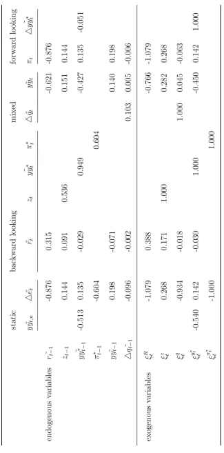
one processes from (96) to (99). The vector of endogenous variables of the system is

xt = [ ˜yyt,n,4e˜t,r˜t, zt,yy˜∗t, πt∗,4q˜t,yy˜t, πt,4yy˜t∗]0. Among the vector,yy˜t,nand4e˜t

are static variables which are just appear at period of timet. ˜rt,zt, ˜yyt∗ and π∗t are

backward looking variables which are appear at period of timet−1 andt. 4q˜tis the

mixed variable which appears at period of timet−1,t andt+ 1. ˜yyt,πt and4yy˜t∗

are forward looking variables which appear at time t and t+ 1. When handling the solution of a dynamic system, it is often replace the static variables with other

endogenous variables so the new vector is Xt = [ ˜rt, zt,yy˜t∗, π∗t,4q˜t,yy˜t, πt,4yy˜t∗]0.

The original system of equations becomes

B[X1,t+1,X2,t+1]0 =A[X1,t,X2,t]0+Gξt+1, (1.100)

where X1,t is the vector of backward looking variables [ ˜rt, zt,yy˜∗t, πt∗]

0 _and _X

2,t

is the vector of mixed and forward looking variables[4q˜t,yy˜t, πt,4yy˜t∗]

0_{. In fact,}

the mixed variable 4q˜t should both enters into the vector of backward looking

(49)

exogenous shocks [ξR

t , ξtz, ξ

q

t, ξ

y∗

t

t , ξ

π∗

t

t ]0. B is a parameter matrix with size 8∗8:

B=                      

1 0 0 (1−ρR)φ4e (1−ρR)()1−α)φ4e −(1−ρR)φy −(1−ρR)(φπ+φ4e) 0

0 1 0 0 0 0 0 0

0 0 1 0 0 0 0 0

0 0 0 1 0 0 0 0

0 0 0 0 1 0 0 0

0 0 0 0 0 1 τ +λ λ_τ

0 0 0 0 αβ 0 β 0

0 0 0 0 0 1 0 −1

                      , (1.101)

and A is a matrix with size 8∗8:

A=                      

ρR 0 0 0 0 0 0 0

0 ρz 0 0 0 0 0 0

0 0 ρy∗ 0 0 0 0 0

0 0 0 ρπ∗ 0 0 0 0

0 0 0 0 ρq 0 0 0

τ+λ −ρz(τ +λ) 0 0 −α(τ +λ)ρq 1 0 0

0 0 −καΘ

τ+λ 0 α −

κ

τ+λ 1 0

0 0 0 0 0 1 0 0

                      , (1.102)

and Gis a matrix with size 8∗5:

G=                      

1 0 0 0 0

0 1 0 0 0

0 0 0 1 0

0 0 0 0 1

0 0 1 0 0

0 0 0 0 0

                      . (1.103)

If the matrixBinvertible, it is appropriate for the Blanchard and Kahn’s

(50)

for the methodology of matrix decomposition to solve the system. The goal of the

solution is to find the transition function:

X1,t =PX1,t−1+Qξt, (1.104)

and the policy function:

X2,t=RX1,t−1+Sξt. (1.105)

After that, it can obtain the static variables yy˜t,n and 4e˜t through the equations

(51)

1.3.1 Blanchard and Kahn’s Methodology

If the inverse of the matrix B exists,the dynamic system (1.100) becomes





X1,t+1

X2,t+1



=B

−1_A



 X1,t

X2,t



+B

−1_G_ξ

t+1. (1.106)

Rewrite B−1_A _{= ΓΛΓ}−1_{.Γ is the eigenvector matrix of the matrix} _B−1_A _{and Λ}

is the eigenvalue matrix. In addition, the eigenvalues follows an increasing order

and the accordingly eigenvectors are also rearranged at the same time. The above

system is rewritten as:

Zt+1 =ΛZt+Γ−1B−1Gξt+1, (1.107)

whereZt =Γ−1Xt. Dividing the eigenvalue matrix in 2 groups based on whether

the absolute value of eigenvalue is smaller or bigger than 1.



 Z1,t+1

Z2,t+1



=





Λ1 0

0 Λ2



 

 Z1,t

Z2,t



+Γ

−1_B−1_G_ξ

t+1, (1.108)

where Λ1 is a submatrix with size Q∗Q and the absolute values of eigenvalues in

it are smaller than 1, while Λ2 is a submatrix with size O ∗O and the absolute

values of eigenvalues in it are equal or bigger than 1. If the system is stationary,

Z2,t = 0 otherwise it explode after infinity time due to the matrix Λ2. Z2,t is also

a matrix with the sizeO∗O. To obtain theX back, rewriting the definition ofZt:



 Z1,t

Z2,t



= Γ

−1

Xt=





G11 G12

G21 G22



 

 X1,t

X2,t



, (1.109)

where the sizes of the sub-matrices in the Γ−1 is [(Q∗m),(Q∗n); (O∗m),(O∗n)] andmandnare the number of variables in the vector ofX1,t andX2,trespectively.

According to the stationary conditionZ2,t = 0,part of the above system becomes:

Z2,t=G21X1,t+G22X2,t = 0. (1.110)

The above equation determines the policy functions of the dynamic system,

cap-turing the relationship between the jump variables and the the predetermined

(52)

solutions to the dynamic system. First, if the number of explosive eigenvalues O is larger than the number of the jump variables n, the system has no solutions. Second, ifO < n,the system has free variables and thus have many infinitely solu-tions. Third, ifO=n, there is one and only one solution for this dynamic system. Overall, if the third condition holds, the unique solution derived from the above

equation is:

X2,t =−G−221G21X1,t. (1.111)

Substitute the unique solution in the rest part of the definition of Zt (1.109),

Z1,t =G11X1,t+G12X2,t, (1.112)

And then substitute it back to the dynamic system (1.108):

G11X1,t+1+G12X2,t+1 = Λ1(G11X1,t+G12X2,t) +Eξt+1, (1.113)

whereE is submatrix of Γ−1B−1Gwith the size m∗6. Substitute the unique solu-tion to the above equasolu-tion and then simplify it to obtain the transisolu-tion funcsolu-tion:

X1,t =RX1,t−1+Sξt, (1.114)

whereR = (−G11G−221G21+G12)

−1

Λ1(−G11G−221G21+G12) and

S = (−G11G−221G21+G12)

−1

E.

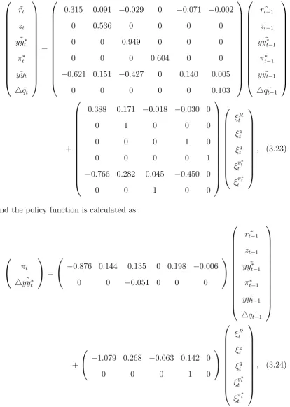
Substitute the transition function to the unique solution to finish deriving the

policy function:

X2,t =P X1,t−1+Qξt, (1.115)