Article
Convolutional neural networks with deep supervised
feature learning for remote sensing scene
classification
Grigorios Tsagkatakis1 and Panagiotis Tsakalides1,2 *
1 Institute of Computer Science, Foundation for Research and Technology-Hellas (FORTH), 70013 Crete, Greece; [email protected] (R.S.); [email protected] (G.T.); [email protected] (P.T.)
2 Computer Science Department, University of Crete, 70013 Crete, Greece
* Correspondence: [email protected]; Tel.: +302811392725
Abstract:State-of-the-artremotesensingsceneclassificationmethodsemploydifferentConvolutional NeuralNetworkarchitecturesforachieving veryhighclassificationperformance. Atraitshared bythemajorityofthesemethodsisthattheclassassociatedwitheachexampleisascertainedby examiningtheactivationsofthelastfullyconnectedlayer,andthenetworksaretrainedtominimize thecross-entropybetweenpredictionsextractedfromthislayerandground-truthannotations.In thiswork,weextendthisparadigmbyintroducinganadditionaloutputbranchwhichmapsthe inputstolowdimensionalrepresentations,effectivelyextractingadditionalfeaturerepresentations oftheinputs.Theproposedmodelimposesadditionaldistanceconstrainsontheserepresentations withrespecttoidentifiedclassrepresentatives,inadditiontothetraditionalcategoricalcross-entropy betweenpredictionsandground-truth. Byextendingthetypicalcross-entropylossfunctionwith adistancelearningfunction,ourproposedapproachachievessignificantgainsacrossawidesetof benchmarkdatasetsintermsofclassification,whileprovidingadditionalevidencerelatedtoclass membershipandclassificationconfidence.
Keywords:Sceneclassification;DeepLearning;ConvolutionalNeuralNetworks;Featurelearning
1. Introduction
Classification of satellite and aerial imagery is a quintessential problem in remote sensing observation analysis. Although the variation in appearance and environmental conditions make this a very challenging problem, in the past few years, machine learning methods have led to a dramatic leap in performance [1,2]. In supervised image classification, both for generic imagery and remote sensing scenes, the current gold standard involves designing an appropriate Convolutional Neural Network (CNN) and training the network so that the cross-entropy loss between the predicted and the ground-truth labels is minimized. The cross-entropy is defined as the KL-divergence between the ground truth labels, encoded as a binary vector where all but one element are zero (one-hot encoding), and the predicted class label distribution from the network, obtained from the last layer after appropriate scaling via a soft-max activation function [3]. Although different loss functions have been proposed for non-classification tasks like focal loss in object detection [4] and mean-squared-error for image enhancement [5], the majority of state-of-the-art CNN architectures employ cross-entropy as the loss function to be minimized for scenarios like supervised image classification [6].
While training a CNN based on the accuracy of the predictions, quantified by the cross-entropy, is a valid and very successful approach, it fails to consider the characteristics of the features extracted by the network. Although feature extraction is an integral part of the CNN classification pipeline, unlike previous state-of-the-art methods that decouple feature extraction and classification, typically,
the outputs of an intermediate layer, relatively close to the output layer, are considered as the features and the final fully connected layer produces the classification results [7]. As such, while end-to-end training of CNNs, using variants of gradient descent, target the minimization of the the classification error, a wealth of information encoded in features extracted from the last fully connected layer, by large, remains untapped.
Motivated by the power of these "features" to encode useful information, in this work we extend the typically CNN architectural pipeline by proposing the addition of an additional output branch that generates low dimensional embedded features extracted from a given input. The proposed scheme, called CNN with Supervised Feature Learning (CNN-SFL) introduces additional terms in the typical loss function which capture the assumption that features extracted from images from the same class when appropriately embedded in a low-dimensional space, must be clustered together. In other words, the feature representation of an example should be close to a representative from the same class and far away from representatives of different classes. As such, the main contributions of this paper are summarized as follows:
• We propose the CNN-SFL, a universally-applicable scheme that can extend and enhance traditional CNN architectures.
• We demonstrate that the proposed scheme achieves better between class separation compared to traditional approaches by employing distances to class representatives.
• We provide experimental evidence that the proposed architecture surpasses, in terms of prediction accuracy, existing state-of-the-art methods, through an evaluation on three benchmark datasets.
• Our analysis also indicates that the proposed scheme is able to provide significantly more separable representations between different classes compared to more traditional approaches.
The remainder of the paper is organized as follows. In Section2, we outline the state-of-the-art in deep learning based remote sensing image classification, focusing on research closely related to the proposed work. In section3we present in detail the proposed CNN-SFL method, while in Section4we report the experimental results and comparisons with state-of-the-art methods. The paper concludes in Section5.
2. Related work
Scene classification represents a critical problem in the domain of remote sensing and numerous approaches have been proposed. In the past five years, the majority of methods considered for this problem employ the deep learning framework and most typically rely on Convolutional Neural Network architectures [1,8], employing categorical cross-entropy for the final class prediction. The idea of introducing the relationship between features in addition to the cross-entropy was considered in [9] where the authors introduced a distance metric loss between the features extracted in the one-before-last layer of a CNN architecture. The core idea of this work is that in addition to minimizing the classification error, the network should also produce features that exhibit low inter-class and high intra-class distances.
In the past few years, different distance metrics have been proposed in the context of Deep Metric Learning [14]. Contrastive loss [15] aims at minimizing the distance between pairs of examples from the same class and maximize the distance between pairs of examples from different classes through the introduction of the appropriate loss function terms using Siamese network architectures. The triplet loss [16] considers triples which consist of a query example, an example from the same class, and an example from a different class. The objective in this case is to minimize the distance between examples from the same class while maximizing the distance between examples from different classes. In [17], K. Sohn proposed the N-pair loss which extended the triplet loss by considering N-1 negative examples simultaneously. The angular loss [18] considers the cosine similarity between examples, and offers scale and rotation invariance.
3. The Convolutional Neural Network with Supervised Feature Learning (CNN-SFL) framework
3.1. Overall CNN-SFL design
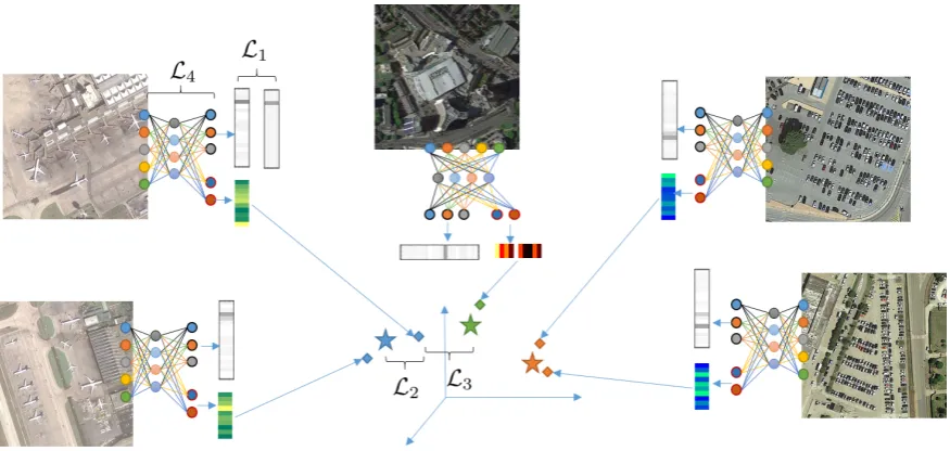
The proposed CNN-SFL is a universal extension of typical CNN architectures for image classification where instead of a single output, the network provides two outputs, one corresponding to the one-hot vector encoding the class predictions, and another providing the low-dimensional features. The key idea behind the CNN-SFL framework, is that traditional CNN architectures seeking to minimize the disparity between predicted and ground-truth classes, can be augmented with an additional constraint enforcing similarity between the feature representations of each example and the associated feature space of representatives corresponding to the same and to different classes. An illustrative block diagram of the propose CNN-SFL framework is shown in Figure1which showcases the three components of the composite loss function, namelyL1,L2,L3representing classification error, distances with between examples and same class representative, and distance to different class representative, respectively.
3.2. CNN-SFL network architecture
LetX= {xi|i= 1, 2,· · ·,N}be a set of Ntraining examples andY = {yi|i =1, 2,· · ·,N}the corresponding classes associated with each example. In our model, we assume that labels are encoded in a one-hot representation such that each labelyi ∈Rcis a vector ofcelements, equal to the number
of classes, has every elements equal to 0 except the one associated with the class of examplexiwhich
is equal to 1. Furthermore, for each example, we associate the features extracted from the network which are given byZ={zi|i=1, 2,· · ·,N}and byC={ci|i=1, 2,· · ·,c}the representatives of the
feature representation of each class. In addition to the representatives for each class, we also define LetLbe the number of layers in the base CNN architecture, i.e., the backbone network. Highly successful architectures which can be utilized as base networks include the ResNet [19] and the Inception [20] architectures. In all these reference architectures, the network consists of L−1 convolutional blocks while theLthlayer is a fully connected (or dense) layer with elements equal to the number of classes. For the specific case of the ResNet, the network consists of a series of convolutional blocks where the input goes through two paths. One path simply propagates the input, while the other consists of a convolution, a batch normalization, a ReLU activation, another convolution and a batch normalization. At the end of the block, these two path are added together and the output goes though a last ReLU activation. For the case of the Inception, each convolutional block consists of multiple independent paths where are all concatenated to product the block output. Exemplary paths include cascade of convolution with different kernel sizes, e.g., 1x1 followed by a 3x3 and then by a another 3x3, or max pooling layer followed by a 1x1 convolution.
For both ResNet and Inception, as well as many other state-of-the-art methods, once the convolutional blocks are calculated, the output is flattened and passed to a fully connected layer where the final layer nodes equal the number of disc int classes. The proposed architecture design, adds an additional fully connected layer ˆL after the(L−1)th convolutional block, such that the network is now equipped with two outputs,LandL. While theLoutput of the network is the same as with other applications and is responsible for producing class probabilities, theLis responsible for the feature embedding process which is utilized by the proposed CNN-SFL in order to estimate the required distances to class representatives.
3.3. CNN-SFL loss function
The objective of the proposed scheme is to minimize the composite loss functionLgiven by
L=L0+λ1L1+λ2L2 (1)
whereL1,L2andL3are the three components of the proposed loss functions, whileλ1andλ2are scaling factors controlling the importance of each component. The first component of the loss function, L1, is the typical cross-entropy between predicted and truth class and is given by
L0=
N
∑
i=1
L(xi)logyi (2)
which is minimized whenL(xi) =yi, i.e., when the predictions, encoded in a one-hot encoding, thus
representing probabilities associated with each class, are in agreement with the ones in the ground truth annotations.
distance between each example and its positive representative, and forL3to maximize the distance between each example and its negative representative.
In order to enforce a small distance between the feature representation of a given exampleiand the corresponding representation of the same class representative, the positive representative, theL2 loss is given by
L1=
N
∑
i=1
exp(kL(ˆ xi)−cik22)−1 (3) where ci is the representative of the features belonging to the same class with examplei. The
additional one is introduced so that the minimum of the loss function approaches zero as the feature representations and the class representatives come closer.
Correspondingly, theL3loss is minimized when the feature representation of an example and the feature representations of the representative from a different class is maximized and is given by
L2=
∑
i
exp(−kL(ˆ xi)−c6=ik 2 2
τ ) (4)
wherec6=iis the closest feature-space representative belonging to a different than the one of example
i. The parameterτ is called the temperature and controlling the impact that the distance has on the value of the loss function term. In both cases, the similarities between feature space examples and the corresponding same and different class representatives are modeled through a radial basis function kernel in order to exploit the properties that the output values of this comparing two vectors is bounded between 0 and 1.
3.4. Class representative selection
In order to select a representative for each class in the feature space, one can consider two scenarios. In the first scenario, the representative corresponds to a "novel" example which is generated by taking the mean of the same class examples in the feature space and is given by:
ci=
1 Nc
Nc
∑
i=1
ˆ L(xi) =
1 Nc
Nc
∑
i=1
zi (5)
whereNcis the number of examples which belong to classc. Another option is to select one of the
training examples as the representative by solving the following minimization problem:
ci =min
Nc
∑
i=1
Nc
∑
j=1,j6=i
kL(ˆ xi)−L(ˆ xj)k2
2 (6)
In addition to the selection of the representative for each class, equally important is the selection of the corresponding negative representative, which is used in Eq. 4. Again, two scenarios can be considered, depending on whether the same negative representative is selected for all the examples in the class, or independent for each example. In the first scenario, the negative representative is the same for all the examples in the same class and corresponds to the representative that is closest to the positive representative for these examples, but from another class. Specifically, once the class representatives are estimated, the negative representative as found by solving:
c6=i=min
Nc
∑
j=1,j6=i
kL(ˆ xi)−L(ˆ xj)k22 (7)
handling the case that some example from a certain class may be closer to a particular negative representative while others may be closes to another negative representative. In this case, the class representatives are estimated by solving:
c6=i=min
Nc
∑
j=1,j6=i
kL(ˆ xi)−L(ˆ xj)k2
2 (8)
In this work, we consider the scenarios where class representatives are estimated and not selected, i.e, we consider Eq.5and Eq.7. We opted for this approach since in the feature space, the estimated representatives capture more realistically the class centroid and are independent of the particular characteristics of the training set.
3.5. Connection to distance metric learning
In the distance metric learning framework, the objective is to estimate a matrixMsuch that the distance between examples from the same classxi,xj is smaller compared to the distance between
examples from different classesxi,xkwhere the distance is computed as the Mahalanobis distance
given by
distM(xi,xj) = (xi−xj)TM(xi−xj). (9)
In order to the metric to be a proper distance, the matrixMmust be positive semi-definite, i.e., all singular values must be XXX. When the matrix entries are real-values, matrixMcan be decomposed using the XX decomposition such that M = QQT where Q is a XX matrix [21]. Given this decomposition, the distance in Eq.9can be equivalently expressed as
distM(xi,xj) =distQ(xi,xj) = (xi−xj)TQTQ(xi−xj) =kQxi−Qxjk22. (10)
In the proposed CNN-SFL, effectively, the feature mapping layer ˆLperform an equivalent function as the matrixQ, albeit employing a non-linear mapping, instead of the linear mapping case whenQis employed. As a results, the new distance considered by the CNN-SLF is given by
distFˆ =kK(F(ˆ xi))−K(F(ˆ xj))k22. (11) whereKis the induced kernel associated with the radial basis function used in Eq.3and Eq.4. 3.6. Comparison with existing approaches
Our work diverges from the approaches proposed in [9] in several ways. First, the proposed scheme can be regarded as an instance of multi-task learning where both a one-hot encoded vector and a feature vector are produced by the network. As such, it offers the flexibility of introducing another distinct path towards the feature space, not necessarily constrained by the given architecture. Second, we extend the idea of imposing constraints on the distances, but instead of considering the distances between examples within a batch, we consider distances between class representatives in feature space, extracted across batches, thus providing greater generalization capabilities. Last, unlike different variance of Deep Metric Learning where the objective is to maximize the similarity between examples from the same class and is thus applicable to retrieval-type settings, the proposed scheme can naturally extent state-of-the-art cross-entropy based classification approaches with the distance learning functionality, thus offering the best of both worlds.
3.7. CNN-SFL training
set, is called an epoch. The proposed CNN-SFL operated in two stages. For each batch, the error of the predicted classes with respect to the ground-truth classes, as well as the distances between the feature space representations and the class representatives are computed and the weights are appropriately updated. This is achieved by computing the gradient of the composite loss as the weighted sum of the individual loss functions. Once all batches have been considered, i.e. after the end of the epoch, the class representatives are re-estimated given the new updated features space mapping. In Algorithm1, we outline the training process of the CNN-SFL.
Algorithm 1CNN-SFL training
Inputs: annotated training examples{xi,yi|i=1, . . . ,N}, pretrained core networkN(0), maximum
number of epochsMaxEpochs, batch sizeB. 1: fort=1, 2, . . . ,MaxEpochsdo
2: forb=1, 2, . . . ,(N/B)do
3: Generate new training set through data augmentation{xi →xˆi|i=1, . . . ,B} 4: Train networkN(t−1)using {ˆx
i,yi,ci,c6=i|i=1, . . . ,B}. 5: end for
6: forj=1, 2, . . . ,Cdo
7: Collect{zk|yk=j}and estimatecjusing Eq.5or Eq.6. 8: end for
9: forj=1, 2, . . . ,Ndo
10: Estimatec6=iusing Eq.7or Eq.8. 11: end for
12: end for
Output: Trained networkN(t)
4. Experimental Analysis
4.1. Datasets and evaluation metrics
In order to understand the behavior of the proposed CNN-SFE scheme, an extensive set of experiments is considered on three representative datasets of aerial imagery, namely the UC Merced [22], the AID [23] and the NWPU-RESISC45 [2].
The UC Merced dataset1 contains aerial color (RGB) images of size 256×256 with spatial resolution 0.3 m from 21 land-use classes including agricultural, airplane, baseball diamond, beach, buildings, chaparral, dense residential, forest, freeway, golf course, harbor, intersection, medium density residential, mobile home park, overpass, parking lot, river, runway, sparse residential, storage tanks, and tennis courts. For each class, the datasets provides a set of 100 images.
The Aerial Image Dataset (AID)2is a large scale collection of 10000 600×600 pixel color images with resolution between 0.5 to 8 m. The images are examples from 30 classes including airport, bare land, baseball field, beach, bridge, center, church, commercial, dense residential, desert, farmland, forest, industrial, meadow, medium residential, mountain, park, parking, playground, pond, port,
railway station, resort, river, school, sparse residential, square, stadium, storage tanks, and viaduct. The number of images for each class varies between 220 and 420.
The NWPU-RESISC45 dataset3contains 31500 256×256 pixel color images at spatial resolution varying between 0.2 to 30 meters. Images at classified into 45 different classes such that each class contains 100 images, while the classes include airplane, airport, baseball diamond, basketball court, beach, bridge, chaparral, church, circular farmland, cloud, commercial area, dense residential, desert, forest, freeway, golf course, ground track field, harbor, industrial area, intersection, island, lake, meadow, medium residential, mobile home park, mountain, overpass, palace, parking lot, railway, railway station, rectangular farmland, river, roundabout, runway, sea ice, ship, snowberg, sparse residential, stadium, storage tank, tennis court, terrace, thermal power station, and wetland.
In the following subsections we investigate the impact that different design choices have on the system’s performance. To that end, we consider images from the AID dataset and a realistic scenario where only 5% of the dataset is available for training, in order to better emphasize the impact of different parameters on the network.
4.2. Impact of feature dimensions
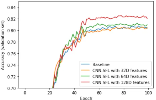
A first aspect we explore regarding the proposed CNN-SLF model is the quantification of the impact that different sizes of the feature space representation have in term of prediction accuracy. Figure2presents the accuracy on the validation set achieved by the baseline ResNet101 model, and the CNN-SFL with ResNet101 as the core network and feature space dimensions equal to 32, 64 and 128. An overall comment from the results presented in Figure2is that the introduction of the additional feature representation module does not reduce the classification accuracy of the standard core model. Examining the different dimensions of the feature space, the results indicate that the 128-dimensional space can have a significant impact in performance, offering gains of more than 3% compared to the baseline mode.
Figure 2.Validation set accuracy as a function of training epoch for the baseline and the proposed CNN-SFL method, considering the values for the feature space representation, namely 32, 64 and 128 dimensional spaces.
4.3. Impact of parameter selection
In order to get a better understanding of the performance of the proposed scheme, we explore the impact of loss function component weighting and impact of temperature parameters. Specifically, in Table1, we explore the impact of weighting between theL1andL2given by parametersλ1andλ2, as well as the temperature parameterτ.
Regarding the impact ofλ1andλ2, an interesting observation is that while their impact in terms of training error is minimal, the performance gains are more pronounced for the testing/validation error. Furthermore, utilizing two loss function components, for intra and inter class similarities, leads to the best performance. Regarding the temperature parameterτ, evidence suggest that their is impact in terms of performance when this value is utilized.
Table 1.Impact of loss component weighting.
Parameter Error
τ λ1 λ2 Training Testing
0.01 10 0 90.47 81.93
0.01 0 10 90.87 81.98
0.01 10 10 90.87 82.42 0.1 10 10 90.87 82.83
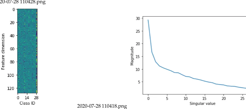
In order to gain a deeper understanding on the behavior of the CNN-SLF, Figure3visualizes the feature-based class representatives in a matrix format and the associated singular values distribution for this matrix. Ideally, one would like class representatives to be as distinct as possible, which in more mathematical way, can be revealed by quantifying the linear dependencies between them. The matrix visualization, but more importantly, the singular values shown in Figure3indicate that class representations from different representatives are relatively orthogonal in the 128-dimensional feature space. As a result, mapping a new test example on this feature space will lead to a representation which is much closer (in terms of projection magnitude) to the a given class representative compared to all others.
2020-07-28 110428.png
2020-07-28 110418.png
4.4. Visualization in low-dimensional spaces
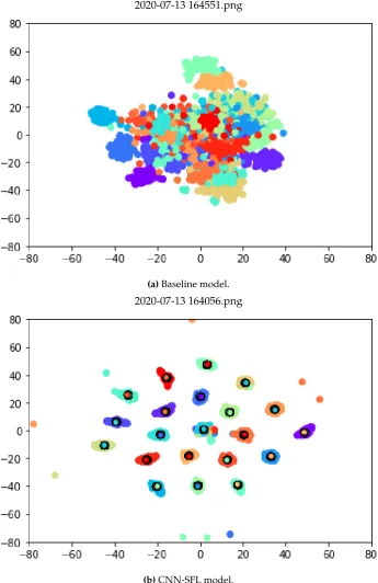
To better understand the impact of the feature embedding module, we employ the t-SNE manifold learning method [24] in order to project the extracted features into 2D spaces and allow the visualization of the outputs. For the case of the baseline network, the t-SNE maps the 2048-dimensional outputs from the first fully connected layer, which is typically considered as the feature representation, while for the CNN-SFL, the mapping is from the 128-dimensional space to the 2Dspace for visualization. The resulting scatter plots are shown in Figure4, the top part for the baseline model and the bottom for the proposed CNN-SLF. In addition to visualizing the extracted features, for the case of the CNN-SLF, we also plot the 128-dimensional feature representations for the class representatives (black circles).
Examining the scatter plots in Figure4, we can clearly see that the separation between different classes achieved by the CNN-SFL is significantly between compared to the baseline model. While for the baseline model, examples from different classes are highly intermingled, for the case of the CNN-SFL, the classes are clearly separated owning to the introduction of theL2loss function (points that are not properly clustered correspond to misclassifications). However, even for the case of samples falling away from their corresponding class region, we observe there are cases where such samples are still closer to their own class region, compared to other class regions. Furthermore, the class representatives are, as expected, centered on the region covered by examples from the corresponding class, indicating theL1loss indeed acts as an attractor.
4.5. Distance based class separation
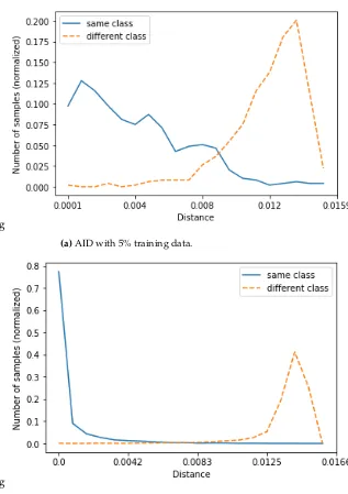
In addition to the classification of imaging using the cross-entropy loss as it is traditionally done, the proposed CNN-SFL framework is also capable of estimating distances between examples and class representatives. To quantify this behavior, Figure5presents histograms of the distance between samples and class representatives from the same and more different classes. Figure5(a) present the histogram for AID with 5% training and and Figure5(b) for UCMD with 80% training data.
In both cases, we observe that distances between representatives from the correct class are in general smaller compared to representatives from the wrong classes. For the case of AID, the two corresponding distributions have some overlap which is a result of misclassification, while for the case of the UCMD which achieves an almost perfect accuracy, there is no observable overlap between the two distributions.
Another observation we can make from these plots is that ideally, all the distances with the correct class representatives should be zero and all the distances with the incorrect classes should have the maximum value. However, the distributions are not delta functions but have significant volume. Even for the case where almost all examples are correctly classified, there is a portion of samples that have a non-zero distance to the correct class representative. This distance can be utilized as a proxy to the confidence associated with each prediction where smaller distances indicate a more reliable prediction. Furthermore, we imposing a threshold between the modes of the same and different class distance distributions, we can allow the network to output "unknown class" responses, unlike traditional cross-entropy-driven CNNs which will always predict a class, even if the particular examples does not belong to the available ones.
4.6. Characteristics of misclassifications
2020-07-13 164551.png
(a)Baseline model.
2020-07-13 164056.png
(b)CNN-SFL model.
Figure 4.2D mapping of samples and class representatives obtained from (a) the ResNet101 baseline model and (b) the CNN-SFL model.
4.7. Comparison with state-of-the-art
2020-07-15 150618.png
(a)AID with 5% training data.
2020-07-16 064427.png
(b)UCMD with 80% training data.
Figure 5.Histogram of distances between samples and representative from the same class (’-’) and from different class (’–’) for AID with 5% training data (a) and for UCMD with 80% training data (b).
CNN architectures, namely CaffeNet [25], VGG-VD-16 [26] and GoogLeNet [27], in addition to two recently proposed methods for scene classification which also consider the notions of distances during classification, specifically, the MDFR [28] and the D-CNN [9].
Figure 6.Confusion matrix for the AID with 50% training data.
Table 2.Classification accuracy for the UCMD dataset.
Method Training ratio
50% 80%
CaffeNet [23] 93.98 95.02 VGG-VD-16 [23] 94.14 95.21 GoogLeNet [23] 92.70 94.31
MDFR [28] - 98.02
D-CNN [9] - 98.93
CNN-SFL (proposed) 97.14 99.29
5. Conclusions
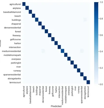
Figure 7.Confusion matrix for the UCMD with 80% training data.
Table 3.Classification accuracy for the AID dataset.
Method Training ratio
20% 50%
CaffeNet [23] 86.86 89.53 VGG-VD-16 [23] 86.59 89.64 GoogLeNet [23] 83.44 86.39 MDFR [28] 90.62 93.37 D-CNN [9] 90.82 96.89 CNN-SFL (proposed) 91.93 94.82
Table 4.Classification accuracy for the RESISC45 dataset.
Method Training ratio
10% 20%
CaffeNet [23] 78.01 81.08 GoogLeNet [2] 82.57 86.02 MDFR [28] 83.37 86.89 D-CNN [9] 89.22 91.89 CNN-SFL (proposed) 90.13 92.27
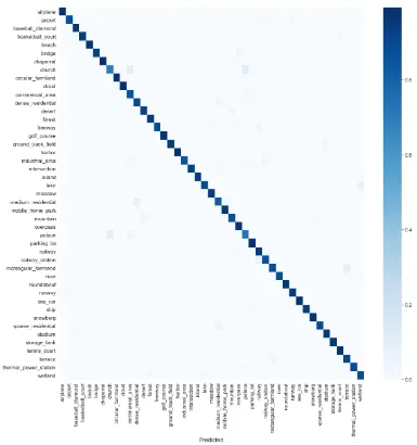
Figure 8.Confusion matrix for the RESISC45 with 20% training data.
Author Contributions:“conceptualization, G.T.; methodology, G.T.; formal analysis, G.T.; writing–original draft preparation, G.T.; writing–review and editing, G.T., P.T..
Funding: his research work work was partially funded by the Marie Skłodowska-Curie CALCHAS project (contract no. 842560) within the H2020 Framework Program of the European Commission and by the Hellenic Foundation for Research and Innovation (HFRI) and the General Secretariat for Research and Technology (GSRT), under HFRI Faculty grant no. 1725 (V4-ICARUS).
Conflicts of Interest:“The authors declare no conflict of interest.”.
References
1. Maggiori, E.; Tarabalka, Y.; Charpiat, G.; Alliez, P. Convolutional neural networks for large-scale remote-sensing image classification.IEEE Transactions on Geoscience and Remote Sensing2016,55, 645–657. 2. Cheng, G.; Han, J.; Lu, X. Remote sensing image scene classification: Benchmark and state of the art.
Proceedings of the IEEE2017,105, 1865–1883.
3. Goodfellow, I.; Bengio, Y.; Courville, A.Deep Learning; MIT Press, 2016. http://www.deeplearningbook. org.
5. Tsagkatakis, G.; Aidini, A.; Fotiadou, K.; Giannopoulos, M.; Pentari, A.; Tsakalides, P. Survey of deep-learning approaches for remote sensing observation enhancement. Sensors2019,19, 3929.
6. Li, Y.; Zhang, H.; Xue, X.; Jiang, Y.; Shen, Q. Deep learning for remote sensing image classification: A survey.Wiley Interdisciplinary Reviews: Data Mining and Knowledge Discovery2018,8, e1264.
7. Gu, J.; Wang, Z.; Kuen, J.; Ma, L.; Shahroudy, A.; Shuai, B.; Liu, T.; Wang, X.; Wang, G.; Cai, J.; others. Recent advances in convolutional neural networks. Pattern Recognition2018,77, 354–377.
8. Zou, Q.; Ni, L.; Zhang, T.; Wang, Q. Deep learning based feature selection for remote sensing scene classification.IEEE Geoscience and Remote Sensing Letters2015,12, 2321–2325.
9. Cheng, G.; Yang, C.; Yao, X.; Guo, L.; Han, J. When deep learning meets metric learning: Remote sensing image scene classification via learning discriminative CNNs. IEEE transactions on geoscience and remote sensing2018,56, 2811–2821.
10. Kang, J.; Fernandez-Beltran, R.; Ye, Z.; Tong, X.; Ghamisi, P.; Plaza, A. Deep Metric Learning Based on Scalable Neighborhood Components for Remote Sensing Scene Characterization. IEEE Transactions on Geoscience and Remote Sensing2020.
11. Boualleg, Y.; Farah, M.; Farah, I.R. Remote sensing scene classification using convolutional features and deep forest classifier.IEEE Geoscience and Remote Sensing Letters2019,16, 1944–1948.
12. Gong, Z.; Zhong, P.; Yu, Y.; Hu, W. Diversity-promoting deep structural metric learning for remote sensing scene classification. IEEE Transactions on Geoscience and Remote Sensing2017,56, 371–390.
13. Yun, M.S.; Nam, W.J.; Lee, S.W. Coarse-to-Fine Deep Metric Learning for Remote Sensing Image Retrieval. Remote Sensing2020,12, 219.
14. Kaya, M.; Bilge, H.¸S. Deep metric learning: A survey. Symmetry2019,11, 1066.
15. Chopra, S.; Hadsell, R.; LeCun, Y. Learning a similarity metric discriminatively, with application to face verification. 2005 IEEE Computer Society Conference on Computer Vision and Pattern Recognition (CVPR’05). IEEE, 2005, Vol. 1, pp. 539–546.
16. Schroff, F.; Kalenichenko, D.; Philbin, J. Facenet: A unified embedding for face recognition and clustering. Proceedings of the IEEE conference on computer vision and pattern recognition, 2015, pp. 815–823. 17. Sohn, K. Improved deep metric learning with multi-class n-pair loss objective. Advances in neural
information processing systems, 2016, pp. 1857–1865.
18. Wang, J.; Zhou, F.; Wen, S.; Liu, X.; Lin, Y. Deep metric learning with angular loss. Proceedings of the IEEE International Conference on Computer Vision, 2017, pp. 2593–2601.
19. He, K.; Zhang, X.; Ren, S.; Sun, J. Identity mappings in deep residual networks. European conference on computer vision. Springer, 2016, pp. 630–645.
20. Szegedy, C.; Vanhoucke, V.; Ioffe, S.; Shlens, J.; Wojna, Z. Rethinking the inception architecture for computer vision. Proceedings of the IEEE conference on computer vision and pattern recognition, 2016, pp. 2818–2826.
21. Suárez, J.L.; García, S.; Herrera, F. A tutorial on distance metric learning: mathematical foundations, algorithms and software.arXiv preprint arXiv:1812.059442018.
22. Yang, Y.; Newsam, S. Bag-of-visual-words and spatial extensions for land-use classification. Proceedings of the 18th SIGSPATIAL international conference on advances in geographic information systems, 2010, pp. 270–279.
23. Xia, G.S.; Hu, J.; Hu, F.; Shi, B.; Bai, X.; Zhong, Y.; Zhang, L.; Lu, X. AID: A benchmark data set for performance evaluation of aerial scene classification.IEEE Transactions on Geoscience and Remote Sensing 2017,55, 3965–3981.
24. Maaten, L.v.d.; Hinton, G. Visualizing data using t-SNE. Journal of machine learning research2008, 9, 2579–2605.
25. Jia, Y.; Shelhamer, E.; Donahue, J.; Karayev, S.; Long, J.; Girshick, R.; Guadarrama, S.; Darrell, T. Caffe: Convolutional architecture for fast feature embedding. Proceedings of the 22nd ACM international conference on Multimedia, 2014, pp. 675–678.
26. Simonyan, K.; Zisserman, A. Very deep convolutional networks for large-scale image recognition. arXiv preprint arXiv:1409.15562014.