New Paradigms for Active Learning

(1)

Western University Western University

Scholarship@Western

Electronic Thesis and Dissertation Repository

8-23-2012 12:00 AM

New Paradigms for Active Learning

Ailing Ni

The University of Western Ontario Supervisor

Charles X. Ling

The University of Western Ontario Graduate Program in Computer Science

A thesis submitted in partial fulfillment of the requirements for the degree in Doctor of Philosophy

Follow this and additional works at: https://ir.lib.uwo.ca/etd

Recommended Citation Recommended Citation

Ni, Ailing, "New Paradigms for Active Learning" (2012). Electronic Thesis and Dissertation Repository. 751.

https://ir.lib.uwo.ca/etd/751

This Dissertation/Thesis is brought to you for free and open access by Scholarship@Western. It has been accepted for inclusion in Electronic Thesis and Dissertation Repository by an authorized administrator of

(2)

NEW PARADIGMS FOR ACTIVE LEARNING

(Spine title: New Paradigms for Active Learning)

(Thesis format: Monograph)

by

(Eileen) Ai-Ling Ni

Graduate Program in Computer Science

A thesis submitted in partial fulfillment

of the requirements for the degree of

Doctor of Philosophy

The School of Graduate and Postdoctoral Studies

The University of Western Ontario

London, Ontario, Canada

c

(3)

THE UNIVERSITY OF WESTERN ONTARIO

School of Graduate and Postdoctoral Studies

CERTIFICATE OF EXAMINATION

Supervisor:

. . . . Dr. Charles. X. Ling

Supervisory Committee:

Examiners:

. . . . Dr. Olga Veksler

. . . . Dr. John Barron

. . . . Dr. Ning Su

. . . . Dr. Steve Wang

The thesis by

(Eileen) Ai-Ling Ni

entitled:

New Paradigms for Active Learning

is accepted in partial fulfillment of the requirements for the degree of

Doctor of Philosophy

. . . . Date

. . . .

Chair of the Thesis Examination Board

(4)

Abstract

In traditional active learning, learning algorithms (or learners) mainly focus on the perfor-mance of the final model built and the total number of queries needed for learning a good model. However, in many real-world applications, active learners have to focus on the learning

process for achieving finer goals, such as minimizing the number of mistakes in predicting unlabeled examples. These learning goals are common and important in real-world applica-tions. For example, in direct marketing, a sales agent (learner) has to focus on the process of selecting customers to approach, and tries to make correct predictions (i.e., fewer mistakes) on the customers who will buy the product.

However, traditional active learning algorithms cannot achieve the finer learning goals due to the different focuses. In this thesis, we study how to control the learning process in active learning such that those goals can be accomplished. According to various learning tasks and goals, we address four new active paradigms as follows.

The first paradigm islearning actively and conservatively. Under this paradigm, the learner

activelyselects and predicts the most certain example (thus,conservatively) iteratively during the learning process. The goal of this paradigm is to minimize the number of mistakes in predicting unlabeled examples during active learning. Intuitively the conservative strategy is less likely to make mistakes, i.e., more likely to achieve the learning goal. We apply this new learning strategy in an educational software, as well as direct marketing.

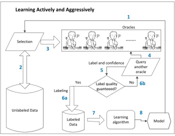
The second paradigm islearning actively and aggressively. Under this paradigm, unlabeled examples and multiple oracles are available. The learner actively selects the best multiple oracles to label the most uncertain example (thus,aggressively) iteratively during the learning process. The learning goal is to learn a good model with guaranteed label quality.

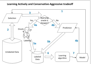
The third paradigm is learning actively with conservative-aggressive tradeoff. Under this learning paradigm, firstly, unlabeled examples are available and learners are allowed to select examples actively to learn. Secondly, to obtain the labels, two actions can be considered: querying oracles and making predictions. Lastly, cost has to be paid for querying oracles or for making wrong predictions. The tradeoff between the two actions is necessary for achieving the learning goal: minimizing the total cost for obtaining the labels.

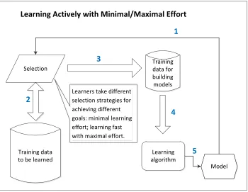
The last paradigm islearning actively with minimal/maximal effort. Under this paradigm, the labels of the examples are all provided and learners are allowed to select examplesactively

to learn. The learning goal is to control the learning process by selecting examples actively such that the learning can be accomplished withminimal effort or a good model can be built fast withmaximal effort.

For each of the four learning paradigms, we propose effective learning algorithms accord-ingly and demonstrate empirically that related learning problems in real applications can be

(5)

solved well and the learning goals can be accomplished.

In summary, this thesis focuses on controlling the learning process to achieve fine goals in active learning. According to various real application tasks, we propose four novel learning paradigms, and for each paradigm we propose efficient learning algorithms to solve the learning problems. The experimental results show that our learning algorithms outperform other state-of-the-art learning algorithms.

Keywords: active learning, learning process, minimizing the number of mistakes, guaranteed label quality, labeling cost, learning effort

(6)

Acknowledgements

My time at Western has been influenced and guided by a number of people to whom I am deeply indebted. Without their help, friendship and support, this thesis would likely never have been finished.

I would like to thank Dr. Charles Ling, my supervisor, who had the greatest impact in my thesis research in the past four years. He had been a tremendous mentor, collaborator and friend, providing me with invaluable insights about research and academic skills in general. I feel exceedingly privileged to have had his guidance.

I thank the examiners of my thesis proposal for their insights and guidance and the profes-sors who gave me great suggestions and help.

Thanks are also given to members of our Data Mining Lab at Western: Da Kuang, Jun Du, Xiao Li, Yan Luo, David deangelis, Arman Didandeh and Nima Mirbakhsh. They are great colleagues and provided me with great help and a friendly environment to work in.

My deepest gratitude and appreciation is reserved for my parents and brothers and sisters-in-law. Without their constant love, support and encouragement, I would never have been able to produce this thesis. I dedicate this thesis to them.

(7)

List of Figures

1.1 Machine learning process. . . 2

1.2 One supervised learning model built on the weather data. . . 3

1.3 Active learning process. The numbers (1-7) indicate the workflow of active learning. . . 5

1.4 The framework of learning actively and conservatively. The learning is an iter-ative process of selecting examples actively to predict. The goal is to minimize the number of mistakes in predicting the unlabeled examples during the learn-ing process. The numbers (1-7) indicate the workflow of the paradigm in each iteration. . . 8

1.5 The framework for learning actively and aggressively with multiple noisy ora-cles. The learning is an iterative process of selecting examples actively to query oracles. For each example, the learner queries different oracles repeatedly until the label quality is guaranteed such that a good model can be built through this learning process. The numbers (1-8) indicate the workflow of the paradigm in each iteration. . . 10

1.6 The framework of learning actively and conservative-aggressive tradeoff. The learning is an iterative process of actively selecting unlabeled examples to query oracle or for prediction depending on their costs. The numbers (1-7) indicate the workflow of the paradigm in each iteration. . . 11

1.7 The framework of learning actively with minimal/maximal effort. The learning is to control the iterative process of selecting examples actively such that the minimal effort is consumed or model can be learned fast by paying maximal effort. The numbers (1-5) indicate the workflow of the paradigm in each iteration. 13 2.1 Zoombinis and their features. . . 20

2.2 Allergic cliffs of Zoombinis game. . . 20

2.3 Screen shot of playing the Allergic Cliff (Zoombinis at the top right corner crossed bridge b1 (top bridge); those at the bottom right corner crossed bridge b2 (bottom bridge)). . . 21

2.4 A case of the Zoombinis game for a human subject. . . 22

2.5 Zoombinis going through b1 (upper) and b2 (lower). . . 23

2.6 Tree model built over the Zoombinis. . . 23

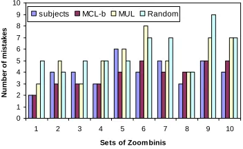
2.7 The number of mistakes on the 10 sets of Zoombini data. . . 25

2.8 The learning efficiency of the three learning strategies. . . 25

2.9 Comparison of the number of mistakes. . . 26

2.10 The number of mistakes . . . 28

(11)

2.11 Performances of models built on the first 12 examples . . . 29

2.12 Mistakes vs. labeled examples . . . 30

2.13 Volatility of learners on UCI datasets. . . 31

2.14 Learning efficiency on UCI datasets. . . 31

2.15 The F measure curves of MCL-1 (with three-step lookahead stopping criterion), MUL and Random. . . 34

2.16 Comparison of the F measure on UCI datasets . . . 34

2.17 Volatility of the F measure on the 10 UCI datasets . . . 34

2.18 The F measure on the marketing data . . . 35

3.1 The basic idea for selecting the best oracle. The decimals in the figure indicate the labeling confidence. . . 40

3.2 Three distributions . . . 44

3.3 Error rate on faithful oracles . . . 45

3.4 The number of examples and label quality of faithful oracles . . . 45

3.5 Error rate on unfaithful oracles . . . 47

3.6 The number of examples and label quality of unfaithful oracles . . . 47

4.1 Probability interval to query oracle. . . 52

4.2 Illustration for action boundary, and the horizontal axis representsP(d|x). . . . 53

4.3 Illustration for indecisive action. . . 54

4.4 Illustration of the learning process for the decisive active learner (DAL). DAL learns the examples in the intervals (shadowed) alternately on the two sides of the action boundaryβ, gradually approachingβ. The actions are taken from the most decisive to the most indecisive. . . 55

4.5 Illustration of the learning process for five learners. DAL is the decisive active learner. IAL is the indecisive active learner learner. AGG is the aggressive learner. CON is the conservative learner. RND is the random learner. . . 59

4.6 Comparison of learning curves in terms of the total cost. Two datasets (anneal and nursery) corresponds to the three rows from left to right respectively. . . 62

4.7 Comparison of learning curves of DAL by using different base classifiers on a dataset (credit-g) under two cost ratios (2.5 and 10). . . 64

5.1 Learning efficiency. . . 78

5.2 The error rate curve vs. iterations of updating models. . . 79

(12)

List of Tables

1.1 A small dataset - weather . . . 3

2.1 The attribute values of the first three Zoombinis in Figure 2.4 . . . 22

2.2 The number of mistakes and the learning sequences of MCL-b, MUL and Ran-dom. . . 24

2.3 Datasets used in the experiments . . . 27

2.4 The ratio of mistakes between MCL and the others . . . 28

3.1 T-test results on 7 datasets with 10 different budgets . . . 46

3.2 T Test results for all datasets and budgets on unfaithful oracles. . . 48

4.1 10 UCI datasets. . . 58

4.2 Statistical comparisons between the five learners in terms of the cost. Each cell shows the average cost and its rank (in the bracket) of a specific learner on a dataset under a cost ratio. The rank is calculated by a statistical test named Wilcoxon signed-rank. In the bottom, the overall average rank and the average rank under the three cost ratios (2.5, 4 and 10) are presented. . . 61

4.3 Comparison of the total cost of DAL by using different base classifiers. In the header, CRatio means cost ratio, BDT represents bagged decision tree, DT rep-resents decision tree and NB reprep-resents naive bayes. The bold value(s) in each row mean that no others are significantly better in that row by using Wilcoxon signed-rank test. . . 65

4.4 Comparison of total cost with different interval-starting strategies. The bold value(s) in each row mean that no others are significantly better in that row by using Wilcoxon signed-rank test. . . 66

5.1 Comparison of error-based effort and size-based effort. In the table, Rnd stands for Random. . . 77

5.2 The comparison of volatility among the three learning algorithms. In the table, Rnd stands for Random. . . 79

5.3 The t-test results on error rate (L: lose; T: tie; W: win). In the table, Rnd stands for Random. . . 80

(13)

List of Appendices

Derivation of Formula 3.1 . . . 93 The Proof of Non-monotonic of Formula 3.1 . . . 94

(14)

Chapter 1 Introduction

In this chapter, we will review some basics of machine learning, supervised learning and tra-ditional active learning first. Then we will state briefly the limitations of the tratra-ditional active learning paradigms, and present an overview of our new paradigms of active learning and the contributions of this thesis.

1.1 Machine Learning

Ever since computers were invented, they have been applied to a wide range of tasks by de-signing and implementing necessary softwares [19, 18]. However, there are many tasks that are difficult or impossible to fulfil by simply programming, as programmers may not be able to anticipate all possible situations and all changes over time or even have no idea on how to program the solution [19, 77]. For example, in speech recognition, it is impossible to map each pronunciation to a word correctly by programming, as the pronunciation of one word varies due to different accents which programmers cannot anticipate. As another example, in detect-ing credit card fraud, even programmers cannot recognize who is a fraud, thus it is impossible to detect fraud by programming.

Naturally experts have been thinking that if computers can be programmed tolearn auto-matically with experience, i.e., making machine learn by itself, the impact would be dramatic. The informal definition oflearninggiven by Tom Mitchell [59] is as follows:

A computer program is said tolearnfrom experienceEwith respect to some class of tasks Tand performance measure P, if its performance at tasks in T, as mea-sured byP, improves with experienceE.

According to the definition, machine learning is to program computers to learn general models from a set of particular examples and optimize their performances.

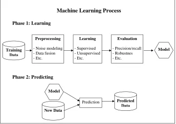
Generally speaking, the machine learning process has two phases, learning and predict-ing, as shown in Figure 1.1. Machine learning researches usually focus on the first phase of learning. As data may be incomplete or come from multiple sources [30], the first step in the phase of learning is preprocessing data, and which is then followed by learning from the data and evaluating the performances of the learned model. In this thesis, we assume that data have

(15)

2 C1. I

Training Data

Preprocessing

- Noise modeling - Data fusion - Etc.

Learning

- Supervised - Unsupervised - Etc.

Evaluation

- Precision/recall - Robustnes - Etc.

New Data

Prediction Predicted

Data

Phase 1: Learning

Phase 2: Predicting

Machine Learning Process

Model

Figure 1.1: Machine learning process.

been preprocessed and we focus on the learning and evaluating steps. The second phase of machine learning is to apply the model learned in the first phase to predicting new data.

Machine learning is clearly meaningful and important, as data are cheap and abundant (data warehouses, data marts), while knowledge (models) is expensive and scarce [11]. According to the important applications on various tasks, machine learning algorithms can be grouped into different types, such as supervised learning, semi-supervised learning, unsupervised learn-ing and reinforcement learnlearn-ing and so on. Among them, supervised learnlearn-ing is an important research area and is useful for numerous applications [48].

1.2 Supervised Learning

Supervised learning is the process of constructing a set of rules, or more generally speaking, creating a model, from examples having both attributes and labels (nominal or numeric). The rules or model is required to achieve minimum error on predicting the labels for future exam-ples drawn independently from the identical distribution (minimum generalization error).

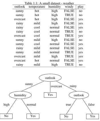
Supervised learning can be illustrated simply with a small set of examples in Table 1.1. The examples have four attributes (outlook, temperature,humidityandwindy) and one label (play

=yesorplay=no). We can build a model with a classical supervised learning algorithm C4.5 [70](see Figure 1.2 for the model).

The decision tree model in Figure 1.2 can be interpreted with a set of rules as follows.

(16)

1.2. SL 3

Table 1.1: A small dataset - weather

outlook temperature humidity windy play sunny hot high FALSE no sunny hot high TRUE no overcast hot high FALSE yes

rainy mild high FALSE yes rainy cool normal FALSE yes rainy cool normal TRUE no overcast cool normal TRUE yes

sunny mild high FALSE no sunny cool normal FALSE yes

rainy mild normal FALSE yes sunny mild normal TRUE yes overcast mild high TRUE yes overcast hot normal FALSE yes rainy mild high TRUE no

outlook

humidity outlook

No Yes

Yes

No Yes

sunny

overcast rainy

high normal true false

Figure 1.2: One supervised learning model built on the weather data.

If outlook=overcast then play=yes; If outlook=rainy and windy=true then play=no; If outlook=rainy and windy=false then play=no.

These rules are meant to be explained in order: the first rule, then if it does not apply then the second, and so on. With the rules, we can predict the label (play=yesorno) for a future example. For instance, given an example, outlook= rainy, temperature= normal, humidity= high and windy=true, we will predict its label asplay=no.

(17)

4 C1. I

have different properties and are suitable for different types of problems. However, in this the-sis, we only focus on different learning paradigms and any supervised learning algorithms can easily be used.

1.3 Active Learning

Traditional supervised learning algorithms have been widely and successfully used in many real applications, such as speech recognition, loan applications, webpage categorization and so on [59, 42, 69]. However, to construct a good model, a considerably large amount of labeled data is usually required, which may be difficult to obtain in real applications. For example, in webpage categorization, each webpage in the training set has to be tagged with certain labels, such as economics, politics, entertainment and so on. This tedious work is usually done manually, and costs a considerable amount of time, human resource and money. Under this circumstance, active learning has been proposed and studied in the past decades.

In active learning, unlabeled examples are assumed to be easily available such as the web-pages on Internet; while the labels of the examples can only be obtained by paying certain cost, such as by paying an expert to label them. Obviously, we can reduce the cost by minimizing the number of examples to be labeled. Instead of obtaining a complete training data passively by traditional supervised learning, active learning selectively obtains the labels of the examples that are most informative for the current model. In this way the final model may be built with fewer labeled examples. Accordingly the cost for labeling examples can be reduced.

Particularly, in active learning, a learner is usually provided with a small (or even empty) set of training examples, and a model is built accordingly. Then the learner selects the most informative example to query an oracle (an expert) for its label and adds the new labeled ex-ample to the training data. By repeating the building-and-querying process, the training set is expanded gradually with informative examples, and the model built from them can be im-proved quickly (i.e., the generalization error on future examples reduces quickly) compared to the “passive” learning. Consequently the number of labeled examples is reduced, and so isthe labeling cost.

Active learning has been widely and successfully applied to many real applications. In the following subsections, we will introduce the commonly used scenarios, query strategies and variants of active learning.

1.3.1 Active Learning Scenarios

Different scenarios have been considered in the active learning research. Two of them are well-studied. One is membership query synthesis [1], and the other one is pool-based sampling [54].

(18)

1.3. AL 5

Unlabeled Data

Labeled Data

Learning algorithm Selection

Model

Active Learning Process

Labeling

1

2

3

4

5 6

Oracle

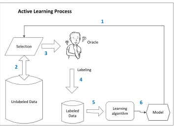
Figure 1.3: Active learning process. The numbers (1-7) indicate the workflow of active learn-ing.

Under the pool-based sampling scenario, in addition to a small (or even empty) set of labeled examples, a large set of unlabeled examples (called “pool”) is given. Usually the unlabeled examples in the pool are assumed to be collected for free or cheaply, such as the webpages and images from Internet. The active learning algorithms select the most informative example from the pool to query an oracle for its label, and update the current model with all the labeled examples. In this way, a good model is expected to be built with fewer labeled examples. In this thesis, the research is under the pool-based active learning scenario, as it is for solving the problems in real-world applications.

In addition to the two scenarios,stream-based selective sampling[14] is also studied in the active learning research. In stream-based selective sampling, unlabeled examples are coming from real data stream (instead of a set of unlabeled examples (“pool”) in pool-based sampling). Each unlabeled example can be observed only for once, and learning algorithms have to decide whether to query it or not based on its informativeness.

1.3.2 Active Learning Query Strategies

As mentioned, to reduce the labeled examples needed, active learning algorithms under the pool-based sampling scenario usually select the most informative example from the pool of unlabeled examples to query. How can we evaluate the informativeness of each unlabeled ex-ample? Many approaches have been proposed for the evaluation, and here we focus on review-ing three commonly used approaches includreview-inguncertain sampling, expected error reduction

anddensity-weighted method.

(19)

6 C1. I

the example that is predicted by the current model with the lowest confidence to query an oracle for its label. For a binary classification problem, uncertain sampling selects the example with predictive probability closest to0.5. The rationale is straightforward: if the current model can predict the example well, then the example does not have much information to improve the model; otherwise, the example is expected to improve the current model effectively.

Expected error reduction is proposed in [76], and it directly focuses on reducing the gener-alization error of the model being built. More specifically, for each unlabeled example xi in a

given pool, the learning algorithm estimates its label and builds a model over the combination of x_i and the training examples. Among them, the example that minimizes the generalization error is selected to query an oracle for its label.

The density-weighted method is proposed by Settles and Craven [85]. The rationale behind this method is that, to reduce the generalization error on the entire example space, the examples from the high density space should be predicted with less error rate. Thus, the unlabeled examples from the high density example space should take precedence over other examples to be queried for labels.

1.3.3 Variants of Active Learning

The query strategies mentioned are to select the most informative example to label such that a good model can be built with fewer labeled examples. The success of the strategies are usually subject to certain assumptions, such as noise-free labels given by an oracle, evenly distributed labeling cost and so on. For solving the learning problems in real applications, different variants, such asactive learning with noisy oraclesandactive learning with variable labeling cost, have been proposed by recent works.

Active learning with noisy oracles is proposed due to the fact that in real applications, noisy labels are ubiquitous. Noise can be introduced to labels by oracles in different ways, such as inaccurate instruments in empirical experiments, distraction or fatigue of experts and so on [83]. The noisy labels affect the active learning performances badly as usually active learning algorithms are noise-prone [3, 97]. To reduce the negative effects, different types of learning strategies have been proposed. One type is focusing on how to select the example that is more informative and less likely to be noisy [3, 25]. The other type is to get rid of the noise in labels by querying multiple oracles [82, 90, 22]. However, label quality still cannot be guaranteed in the previous works. In this thesis, we will study how to remove the noise and guarantee label quality in Chapter 3 with multiple oracles.

Active learning with variable labeling cost tries to solve the problems that the labeling cost is example-dependent or oracle-dependent. For example-dependent labeling cost, two groups of active learning strategies have been proposed. One is that the labeling cost is known before selecting the examples (e.g., [46, 47]). The other group is to handle the problem that the costs for labeling examples are variable and unknown [86]. For oracle-dependent labeling cost, learning strategies have been proposed in [110, 21] to select low-cost combinations of oracles that result in high-accuracy labels of examples. As a result, the total cost in building a good model can be minimized.

(20)

1.4. NP AL: O 7

machine learning researches, such as active clustering [43, 7], active transfer learning [91], active feature acquisition and classification [58, 78], active class selection [55] and so on.

1.3.4 Limitations of Traditional Active Learning Paradigms

Active learning has been fairly well-established in theoretical research and various real-world applications. Most of the active learning research has concluded with encouraging results that the number of queries can be reduced by querying oracles actively (e.g., [81, 54, 32, 41]). However, some previous works [80, 39, 86, 4] also show the limitations of active learning on some circumstances, such as alternative query types and so on. This may be due to the many simplified assumptions in previous works [81]. In this thesis we address two types of new and different limitations.

The first limitation is that most traditional active learning paradigms only focus on the num-ber of examples labeled (queries issued) and the prediction accuracy of the final model built. However, they do not study learner’s performances during the learning process which in fact is very important. For example, in directed marketing (a process of identifying likely buyers to market products actively), sales agents need to select and approach the “right” customer (the customer who will buy the products). Obviously its final goal is to make fewest mistakes dur-ingthe selection (learning) process, rather than the high prediction accuracy of the final model as in traditional active learning (See Chapter 2 for further discussion). As another example, human often prefers taking minimal effort during the process of learning new knowledge. It is also crucial to minimize the machine learning effort during the learning process as effort is related to energy consumption, system reliability and so on (See Chapter 5 for further discus-sion). The traditional active learning does not study those goals in the process of learning, as we do in this thesis.

The other limitation is that the label quality in active learning cannot be guaranteed. Most traditional active learning paradigms assume that oracles are always correct. However, noise can be introduced to labels in different ways as mentioned in Section 1.3.3. To rule out the negative effects of the noisy labels, multiple imperfect oracles are used in previous works [82, 90, 22]. By querying multiple oracles for each example, the final label obtained is expected to be more accurate. This multiple-oracle strategy is reasonable and useful in improving label quality. However, there is still no way to guarantee the label quality. We will propose a novel learning paradigm in Chapter 3 to overcome the limitation.

1.4 New Paradigms of Active Learning: an Overview

(21)

8 C1. I

1.4.1 Learning Actively and Conservatively

The new paradigm of learning actively and conservativelyis proposed to study the learning processes that the traditional active learning ignores. More specifically, it focuses on the learn-ing process of selectlearn-ing unlabeled examples gradually, and tries to reduce the number of mis-takes that the learner makes in predicting them. The learning process is important in many real-world applications. Taking the direct marketing as an example again, to make the market-ing more efficient, a learner (or an agent) has to focus on the selection process and tries to find and approach the “right” examples (customers) [106]. Accordingly the number of mistakes made during the learning process is reduced.

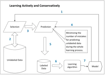
The proposed paradigm of learning actively and conservatively (see Figure 1.4 for its frame-work) is applicable for the problems that are of the following settings. First of all, unlabeled examples are provided and learners can actively select examples from them (Steps 1 and 2 in Figure 1.4). This is the same as traditional active learning. In the direct marketing example, all the customers are unlabeled (not knowing who is “buying” and who is “not”), and a sales agent can select the customers to approach. Secondly, the selected unlabeled examples are predicted by the learner itself, and the true label is revealed after each prediction (Steps 4 and 5). In direct marketing, the true label of a customer (”buying” or ”not buying”) is revealed after a learner (an agent) approaches a predicted buyer. The goal of this paradigm is to minimize the number of mistakes for predicting unlabeled examples during the iterative learning process.

Unlabeled Data

Labeled Data

Model

Learning Actively and Conservatively

Prediction

1

2

3

4

5

6 7

Minimizing the number of mistakes for predicting unlabeled data during the whole learning process.

Figure 1.4: The framework of learning actively and conservatively. The learning is an iterative process of selecting examples actively to predict. The goal is to minimize the number of mistakes in predicting the unlabeled examples during the learning process. The numbers (1-7) indicate the workflow of the paradigm in each iteration.

(22)

1.4. NP AL: O 9

be solved by the traditional active learning algorithms. To fill the gap, we propose a new and effective algorithm calledMost-Certain Learning(MCL). The basic idea of MCL is to select the next unlabeled example that can be predicted by the learner with the highest certainty (thus, it is conservative). The rationale behind is that learning is a gradual process, and the uncertain examples can become certain ones with more examples being learned. In this way, the goal of minimizing the number of mistakes during the learning process can be achieved.

In our empirical study, first of all, we apply MCL to an educational game Zoombinis, which is a learning problem under the paradigm of learning actively and conservatively (see Section 2.3.2 for the details), to illustrate the learning process of MCL. Then we also apply MCL to both UCI [2] datasets and one real-world application, direct marketing. The experimental results show that MCL works much better than other learning strategies. Furthermore, we also discover another advantage of MCL: the learning process is much more stable than other learning strategies. This property is often important as it makes the learning behavior more predictable. See Chapter 2 for detailed studies on this learning paradigm.

1.4.2 Learning Actively and Aggressively

To the opposite of the paradigm of learning actively and conservatively, traditional active learn-ing algorithms with uncertain sampllearn-ing are under the paradigm oflearning actively and aggres-sivelyas they usually select the example that is predicted with the least certainty (i.e., aggres-sively) to query an oracle. Under this paradigm, the goal is to build a good model with as few labeled examples as possible. However, in traditional active learning, the label quality cannot be guaranteed as oracles are usually imperfect and the noisy labels of examples deteriorate the learning performances badly.

To guarantee the label quality, we use multiple imperfect oracles which are able to return both labels and their confidences in the labels (see Figure 1.5 for the framework). In fact, this circumstance exists commonly in real-life. For example, in paper reviewing, multiple reviewers (i.e., oracles or labelers) are requested to label a paper (as accepted, weak accepted, weak rejected or rejected), and usually the reviewers are required to give not only labels (accept, weak accept, weak reject or reject) for the paper, but also their confidences (high, medium or low) for the labelings. With the labels and confidences given by oracles, the final label (decision) quality can be estimated and guaranteed by querying more oracles if needed (see Steps 4, 5 and 6b in Figure 1.5).

Under this paradigm, we propose a new active learning strategy, called c-certainty label-ing. C-certainty labeling guarantees the label quality to be greater than or equal to a given threshold c (c is the probability of correct labeling; see Section 3.2). Furthermore, instead of assuming noise level to be example-independent in the previous works, we allow it to be example-dependent. Our learning algorithm selects the best oracles to query for each given example. Thus, fewer queries are required on average for a label to meet the thresholdc com-pared to random selection of oracles. As a result, for a given query budget, a more accurate model can be built with our learning algorithm.

(23)

10 C1. I

Unlabeled Data

Labeled Data

Model

Learning Actively and Aggressively

Labeling

…….

Label quality guanteeed? Label quality

guanteeed?

Yes No

Label and confidence Query

another oracle

1

2

3

4

5

6a

7 8

6b

Oracles

Figure 1.5: The framework for learning actively and aggressively with multiple noisy oracles. The learning is an iterative process of selecting examples actively to query oracles. For each example, the learner queries different oracles repeatedly until the label quality is guaranteed such that a good model can be built through this learning process. The numbers (1-8) indicate the workflow of the paradigm in each iteration.

detailed studies of this learning paradigm).

1.4.3 Learning Actively with Conservative-Aggressive Tradeo

ff

In the paradigm of learning actively and conservatively, learners always predict unlabeled ex-amples during the learning process. On the other hand, in the paradigm of learning actively and aggressively, learners always query oracles for the labels. However, in many real-world applications, labels can be acquired by either querying oracles or making predictions. For ex-ample, when letters are sorted by using OCR (optical character recognition) devices of the post office, if the hand-written postal codes are ambiguous, or too difficult to recognize, they will be passed to the oracles (human) for labeling (i.e., querying oracles). However, if the OCR can predict accurately the hand-written postal codes, the letter will be sorted and mailed to the recipient directly (i.e., predicting directly) even though there is a small chance the prediction is wrong. To handle this type of learning problems, we propose a new paradigm oflearning actively with conservative-aggressive tradeoff (as shown in Figure 1.6) such that the correct actions (predicting or querying) can be taken during the learning process.

(24)

1.4. NP AL: O 11

Unlabeled Data

Labeled Data

Model

Learning Actively and Conservative-Aggressive tradeoff

Labeling

Querying oracle is cheaper? Querying oracle is cheaper?

Prediction No

Yes

1

2

3

5a 5b

6 7

Oracle

4a 4b

4b

Figure 1.6: The framework of learning actively and conservative-aggressive tradeoff. The learning is an iterative process of actively selecting unlabeled examples to query oracle or for prediction depending on their costs. The numbers (1-7) indicate the workflow of the paradigm in each iteration.

two actions can be considered: querying oracles (e.g., asking human and experts) or making predictions (e.g., predicting mails by OCR directly). Lastly, cost has to be paid for making a wrong prediction or for querying an oracle. To reduce the cost, the choice of actions depends on the expected cost for making a wrong prediction (Ce) and the cost for query an oracle (Cq). For

example, ifCe >Cq, the learner will choose to get the label by querying an oracle; otherwise,

the learner will choose to predict its label directly. The selection of the two actions is optimal (i.e., obtaining the labels with minimal total cost) if the estimation ofCeis correct.

However, the expected costCemay not be very accurate particularly in the beginning of the

learning process as the model is not good enough. For the example that its expected costCeis

close to query costCq, it is likely that a wrong action will be taken, which may consequently

lead to a high cost. On the other hand, wrong actions will unlikely be taken for the example that itsCeis much higher or much lower thanCq.

Considering the two actions and their different costs, we propose a novel learning algo-rithm, calledDecisive Active Learner (DAL), which always selects the example likely leading to correct actions and prefers the action that is expected to cost less during the learning process. The examples that will likely lead to wrong actions will be learned during the later stage, as the learner may become more reliable (the probability is more accurate) and the action taken will become more accurate with more example being learned.

(25)

12 C1. I

cost settings. See Chapter 4 for detailed study on this learning paradigm.

1.4.4 Learning Actively with Minimal

/

Maximal E

ff

ort

In addition to the paradigms mentioned to improve the performances of learners on different goals, we also consider the relations between the performance of a learner on achieving learn-ing goals and theeffortthat the learner takes during the learning process. Intuitively the effort can be reflected by the energy consumption of machine learning algorithms. As energy con-sumption can be affected by many factors such as processor speed, monitor size, we will use the amount of error to be corrected during learning, and the size of the learning models, to approximate the effort.

In fact, theeffortof active learning can correspond well to the actual effort in human learn-ing, where two circumstances are usually studied. One is learning knowledge with minimal effort. It is supported by an “i+1” education theory which suggests that less effort is required for human learning a small piece of new knowledge (“1”) based on a large body of previously learned knowledge (“i”)[49]. The other circumstance is that learning can be more efficient by paying maximal effort on correcting mistakes. It also has been studied in psychology and education in the past [105, 67].

The two circumstances of human learning researches are also important in the process of building machine learning modules. More specifically, in machine learning, minimal effort in-dicates consuming minimal energy during the learning process. Energy consumption control-ling is very important[60], and when modules consume more energy they must be aggressively cooled or batteries will die sooner [45]. On the other hand, learning efficiency is also crucial for machine learning problems as tremendous data are collected everyday.

To study this learning effort problem, we propose a new paradigm of learning actively with minimal/maximal effort. In this paradigm, the labels of the examples are all provided and learners are allowed to select examples actively to learn. The learning goal is to control the learning process by selecting examples actively such that the learning can be accomplished with minimal effort or good models can be built fast with maximal effort. The framework of the paradigm is shown in Figure 1.7.

For the minimal effort learning, we propose an effective learning algorithm Simple-to-Complex (S2C). The basic idea of S2C is to repeatedly select and learn the example that its prediction given by the current learner is the closest to the true label (i.e., the simplest exam-ple) during the learning process. The rationale behind this greedy algorithm is that the complex examples will become simpler with more examples being learned. In this way, the learning ef-fort can be minimized for the whole learning process.

On the other hand, for maximal effort learning, we repeatedly chose to learn the example that its prediction is the most different from the true label during the learning process. Due to the largest difference, the example is expected to be the most informative for the learner. In this way, it can improve the learner the most, and the learning is expected to be the most efficient.

(26)

1.5. C  T 13

Training data to be learned

Model Learning Actively with Minimal/Maximal Effort

Training data for building models

1

2

3

4

5

Learners take different selection strategies for achieving different goals: minimal learning effort; learning fast with maximal effort.

Figure 1.7: The framework of learning actively with minimal/maximal effort. The learning is to control the iterative process of selecting examples actively such that the minimal effort is consumed or model can be learned fast by paying maximal effort. The numbers (1-5) indicate the workflow of the paradigm in each iteration.

1.5 Contributions of the Thesis

Traditional active learning has been extensively studied on learning a better model with fewer labeled examples compared with traditional supervised learning. However, limitations exist when the traditional active learning algorithms are applied to real applications, as mentioned. To fill the gap, we propose four novel active learning paradigms based on the requirements of real applications. The contributions of this thesis can be summarized as follows.

• We propose a new learning paradigm, learning actively and conservativelyin Chapter 2. Under this paradigm, learners actively select examples to learn, but their behavior of selecting examples is conservative in order to minimize the error in predicting examples. The learning algorithm is called MCL (Section 2.2) which prefers to learn the example that can be predicted with the highest certainty. This work is published inThe Proceed-ings of International Conference on Artificial Intelligence and Education (ICAIE), 2010

[63]

(27)

14 C1. I

proposed does reduce the number of mistakes in predicting unlabeled examples during the learning process. MCL-1 is for retrieving the examples of one class in Chapter 2.4. The experiments are conducted on both UCI datasets and a direct marketing dataset. The results show that our learning algorithm works well on all the datasets, and our learning algorithm does select more customers who will buy products than other learning algo-rithms. This work is published in The 7th International conference on Advanced Data Mining and Applications (ADMA’11)[62].

• The second paradigm islearning actively and aggressivelyin Chapter 3. It selects exam-ples actively and aggressively to learn, which is the same as traditional active learning. However, traditional active learning algorithms cannot guarantee label quality as oracles may not be always correct. We extend this learning paradigm by asking oracles to pro-vide both labels and confidences. With this extension, we guarantee label quality to be higher than a given thresholdc. In addition, an efficient learning algorithm is proposed to select the oracles with high labeling confidence to query. Extensively empirical stud-ies are conducted on UCI [2] datasets. This work is published in The 16th Pacific-Asia Conference on Knowledge Discovery and Data Mining. May, 2012[64].

• The third paradigm proposed is called learning actively with conservative-aggressive tradeoff in Chapter 4. Under this paradigm, to obtain labels, learners are allowed to take two actions: predicting directly by its current model or querying an oracle. The decision on taking which of the two actions depends on the expected cost for predicting and the cost for querying an oracle. To minimize the total cost, we proposed a novel learning algorithm, Decisive Active Learner (DAL), which prefers to learn the example that its action is more likely to be correct. Empirical study is conducted extensively on UCI dataset and the results show that DAL does work well. This work is submitted to The IEEE International Conference on Data Mining (ICDM), 2012.

(28)

Chapter 2 Learning Actively and Conservatively

In traditional active learning, learners only focus on the number of queries issued and the performances of final models learned. However, they ignore the performances of learners during the learning process. In this chapter, we propose a new paradigm oflearning actively and conservativelywhich focuses on the process of learners selecting examples iteratively to learn and tries to make as few mistakes as possible in predicting unlabeled examples during the learning process.

The learning process is important for many applications. For example, in direct marketing, a sales agent (learner) has to focus on the process of selecting customers to approach, and tries to make correct predictions (i.e., fewer mistakes) on the customer who will buy the product. As another example, a doctor has to focus on the process of diagnosing each patient and tries to predict correctly. This type of learning problems are under the paradigm of learning actively and conservatively.

In general, the problems under the paradigm proposed have specific settings as mentioned in Section 1.4.1. One is that unlabeled examples are available for learners to select actively. This is the same as traditional active learning. The other one is that the selected example is predicted by the learner and the true label will be revealed after each prediction. In the direct marketing example, the true label of a customer (“buy” or “not buying”) will be revealed after an agent predicts him/her as “buying” and approaches. The goal of the learning paradigm is to minimize the number of mistakes in predicting unlabeled examples during the iterative learning process.

Under the paradigm of learning actively and conservatively, we propose a new, practical and effective learning algorithm, Most-Certain Learning (MCL). To minimize the number of mistakes, MCL chooses to learn the next example whose label can be predicted by the current learner with the highest certainty. This work of MCL is published in The Proceedings of International Conference on Artificial Intelligence and Education (ICAIE), 2010[63].

Furthermore, to satisfy the requirements of real-world applications, we further discuss two types of MCL. One is that the learner must select and predict all of the remaining examples as either positive or negative classes, calledbinary-class MCL, orMCL-b. The goal of MCL-b thus is to minimize mistakes of MCL-both classes. For example, a doctor usually must see and diagnose all patients as healthy or sick. The other type is that the learner only needs to select and predict one class of examples, calledsingle-class MCL, orMCL-1. In the direct marketing example, an agent usually only cares about those customers who will likely buy the product

(29)

16 C2. LA C

(positive examples), and does not need to predict, approach, and verify customers who will unlikely buy the product (negative examples). This work is published onThe 7th International conference on Advanced Data Mining and Applications (ADMA’11)[62].

The rest of this chapter is organized as follows. Section 2.1 reviews related works. Section 2.2 describes the framework of the Most-Certain Learning (MCL) strategy. Section 2.3 and Section 2.4 present the details of implementing the two versions (MCL-b and MCL-1) of MCL and present their experimental results respectively. We summarize the work of this chapter in Section 2.5.

2.1 Related Works

The paradigm of learning actively and conservatively is an active learning paradigm in the sense that it allows learners to select examples actively to learn. However, existing active learning algorithms [82, 15] cannot solve the problems under the paradigm as their settings and goals are different. The traditional active learning targets on minimizing the number of examples labeled and the high prediction accuracy of final models; while our paradigm is to minimize the number of mistakes in predicting unlabeled examples during the learning process. Furthermore, in the traditional active learning learners can only get labels by querying oracles; while under our paradigm, examples are predicted by learners and the true labels will be revealed after each prediction.

The learning problems under our paradigm may seem to be similar to agnostic active learn-ing [3, 16] as both of them are related to mistakes in labels. However, the noise in agnostic active learning comes from the oracle who provides the labels, and the true labels are hidden. The goal of agnostic active learning is to improve the sample efficiency. For our learning prob-lem, the mistakes come from the prediction of the current immature learner and the true label will be revealed after the prediction, and the goal is also different.

Another work that is quite similar to our work is self-directed learning [9, 38, 75]. The-oretically it studies the learning problem on simple classes of concepts, such as disjunction, conjunction, k-DNF and so on, to minimize the number of mistakes. However, the learning algorithm proposed must know and keep the set of all target concepts. It chooses the next example that has the greatest difference between the number of concepts that predict it diff er-ently (positive vs. negative labels). In a sense, the algorithm chooses the example that can be predicted most certainly. However, the target concept class is often unknown, nor is it feasi-ble to keep all the concepts for a learning algorithm in real-world applications. As far as we know, there is no previous work in designing a practical learning algorithm that works well (i.e., making fewer mistakes) for solving the problems under the paradigm of learning actively and conservatively.

2.2 Most-Certain Learning (MCL) Strategy

(30)

2.2. M-CL(MCL) S 17

be predicted by the current learner with the highest certainty first, and leave the examples with low certainty to learn during the later stage. One might think that the total number of mistakes would be the same no matter what order of examples to be selected. Afterall, all unlabeled examples need to be learned, from easy to complex or from complex to easy ones. It is analo-gous to 1+2+3= 3+2+1. However, we will show that the learning sequence does matter. The rationale behind is that, with more examples being learned, the prediction accuracy of the learner can be improved, and consequently uncertain examples can become certain. In this way, the goal of minimizing the number of mistakes in predicting unlabeled examples can be achieved. In particular, MCL can be defined formally as follows.

LetD_Ube the unlabeled example set, andCbe the concept class overD_U. MCL focuses on the iterative learning process as follows: in each iteration, it chooses a new element (example)

x_i ∈ D_U that can be predicted by the current learner L with the highest certainty. It then outputs the label l_i given by L and in response the true value ct(xi) will be revealed, where

ct (ct ∈ C) denotes the target function. The learner will update its current model with all the

labeled examplesD_T. The learning process continues until all the elements inD_U are learned or other stopping criteria are met. Letm(L,ct) denote the number of mistakes made byL, i.e.,

the total times ofli , ct(xi). The goal of MCL is to minimizem(L,ct). The pseudocode for

MCL is shown in Algorithm 1.

Algorithm 1: MCL

Input: Unlabeled DatasetD_U; Training data: D_T; Initial model:M₀

Output: Model: Mand the number of mistakes: m

begin

1

itr= 0;//the first iteration

2

m=0;

3

whileD_U <>NU LLdo

4

foreach x_i ∈ D_U do

5

Calculate the certainty of xi;

6

end

7

//Select the most certain example

8

Select the example xiwith the highest certainty;

9

l_i ←label prediction of x_i;

10

ct(xi)←the true label ofxi;

11

ifli , ct(xi)then

12

m= m+1;

13

end

14

D_T ← D_T +xi;

15

Update the current model withD_T;

16

D_U ← D_U−x_i;

17

itr+ +;

18

end

19

M ← M_itr;

20

ReturnMandm;

21

end

(31)

18 C2. LA C

MCL is a wrapper learning algorithm, and can take any classifier that generates delicate probability prediction as its base learner,L. In this paper, bagged decision trees [71] are taken as the base learner for two reasons. First of all, it is easy to obtain an accurate probability of the prediction. The second reason is that a large number of empirical studies in machine learning have shown that bagged decision trees make classification more accurately compared to a single tree [8, 71].

MCL provides a framework for solving problems under the new paradigm. According to the diverse learning problems in real-world applications, we further implement two types of MCL. One type is that learners must select and predict all of the remaining examples as either positive or negative class1, called binary-class MCL, or MCL-b. The goal of MCL-b thus is to minimize the number of mistakes on both classes. For example, in the Zoombinis game mentioned in Chapter 1 (for details see Section 2.3.2), a player has to label a Zoombini (a small creature) with either of the two bridges. As another example, a doctor usually must see and diagnose each patient as healthy or sick. The other type is that learners only need to retrieve one class of examples, calledsingle-class MCL, orMCL-1. In the direct marketing example, an agent usually only cares about those customers who will likely buy the product (positive examples), and does not need to predict, approach, and verify customers who will unlikely buy the product (negative examples).

2.3 MCL-b Learning Algorithm

MCL-b works under the framework of MCL as follows. It selects the most certain example of

bothclasses and predicts it with its current model. Then MCL-b updates its current model with the newly labeled example. This predicting-and-updating process iterates until all the examples are labeled.

In this subsection, first of all we will introduce the implementation details of MCL-b. Then we will present how MCL-b works and its performances on an educational game Zoombinis. After that, we will show the experimental results of MCL-b on UCI [2] datasets extensively.

2.3.1 MCL-b Implementation Details

To implement MCL-b, three technical issues deserve extensive discussion. The first issue is the selection of the most certain example. The second issue is the selection of the first example. The last issue is how to select an example when the labeled examples are of the same class.

The first issue, selection of the most certain example, is crucial. The most-certain example is the one that is predicted with the highest probability by the current learner, i.e., the example that satisfies arg max

x_i∈X

(max(prob+_x

i,(1− prob

+

x_i))). prob+x_i is the probability of predicting xi as

positive. In bagged decision trees (which is used as our base learner), prob+_x

i is the number of

decision trees that vote for positive out of the total number of decision trees.

The second issue, the selection of the first example, can be tricky, as the current model is empty. MCL-b scans the dataset and chooses the example that appears with the highest

1_{This study assumes that the learning problem is binary-class. The multi-class problem can be transformed to}

(32)

2.3. MCL-LA 19

frequency. If no example appears more than once, MCL-b chooses one example from the dataset randomly.

The last issue is how to choose the next example if labeled examples so far are of the same class, as a model built from the examples of the same class, say positive, will predict all examples as positive. Here, we use the Euclidean distance [92] as heuristic information for selecting the next example. The basic idea is that the example far from a positive (negative) center is likely negative (positive). Assuming that MCL-b has a positive example x₁ with nominal attribute values{1, 0, 0, 1}, we consider it as the center of positive, and the point that has the furthest Euclidean distance from x1 (here the possible furthest Euclidean distance is4)

as the center of negative. The most certain example is the one that is closest to either of the two centers, and the label of the center will be assigned to the example. For example, if the nearest example fromx1isyu, and the Euclidean distancedx₁y_u =1, and the furthest isyv, and

dx₁yv =4, MCL-b would consideryvas the most certain example and label it as negative. The

reason is thatyvhas distance0to the negative center, which is closer than the distance ofyu to

the positive center. This strategy can be formulated as follows.

y=

(

yu, ifPx_i∈S dx_iyu < |S| ∗m−Px_i∈S dx_iyv

yv, otherwise (2.1)

whereS is the set of labeled examples,|S|is the size ofS,mis the number of attributes,dx_iyuis

the Euclidean distance between xi andyu, andyu andyvare the closest and furthest unlabeled

examples to the current labeled examples respectively.

After presenting the implementation techniques, we will show how MCL-b works on a learning problem (an educational game Zoombinis) under the paradigm of learning actively and conservatively. Then we will present the performances of MCL-b in playing the game. Furthermore, extensive empirical studies on UCI [2] datasets will also be conducted.

2.3.2 Application in the Educational Game Zoombinis

MCL-b can be applied to many real-world learning problems under the paradigm of learning actively and conservatively, even including some human concept learning problems. In this section, we apply the machine learning algorithm MCL-b to an educational game, Zoombinis, to illustrate how it works and show its performances on this learning problem.

The game Zoombinis is a well-known series of software published by the Learning Com-pany2. It aims at children or teenagers, but fun for adults as well. It is based on the “Zoombi-nis”, small blue creatures, which are depicted with varying hairs, eyes, noses and feet. Figure 2.1 shows three Zoombinis and possible feature values. In the Logical Journey of the Zoom-binis game, ZoomZoom-binis have to search for a new home, and on their journey they encounter a variety of “obstacles” (puzzles), which players must solve. In this experiment, we choose one puzzle, called the Allergic Cliffs, to work on.

In the Allergic Cliffs (Figure 2.2), the player is given 16 randomly-generated Zoombinis. The goal is to take all of the 16 Zoombinis across the cliff to the right side over the two bridges. The two bridges are supported by 6 wooden pegs. Each bridge allows only certain

2_{There are three titles in the series: The Logical Journey of the Zoombinis, Zoombinis: Mountain Rescue, and}

(33)

20 C2. LA C

Hair=small, Eyes=glasses, Noses=green, Feet=springs

Hair=short, Eyes=wide open, Noses=orange, Feet=two wheels

Hair=flat-topped, Eyes=sun glasses, Noses=red, Feet=rollers

Hair (shaggy, ponytailed, flat-topped, small, and short)

Noses (green, orange, red, purple and blue)

Eyes (wide open, one eyed, half-closed, glasses and with sunglasses)

Feet (shoes, rollers, springs, two wheels and propellers)

(a) Three Zoombinis

Hair=small, Eyes=glasses, Noses=green, Feet=springs

Hair=short, Eyes=wide open, Noses=orange, Feet=two wheels

Hair=flat-topped, Eyes=sun glasses, Noses=red, Feet=rollers

(b) Zoombinis’ features

Figure 2.1: Zoombinis and their features.

Six wooden pegs

(34)

2.3. MCL-LA 21

Figure 2.3: Screen shot of playing the Allergic Cliff(Zoombinis at the top right corner crossed bridge b1 (top bridge); those at the bottom right corner crossed bridge b2 (bottom bridge)).

Zoombinis to cross if they have certain combinations of features. The pattern (model) for each bridge is randomly formed and hidden to the player. For example, the top bridge may only allow Zoombinis with red or blue nose to cross (and thus, the bottom bridge allows all other Zoombinis to cross). If the player selects a Zoombini to cross a wrong bridge, the cliffwould sneeze, the Zoombini will be sent back to the left side, and a peg will spring loose by the powerful sneeze. Figure 2.3 is a screen shot in taking the Zoombinis in Figure 2.2 across the cliff. We can see that two pegs have sprung loose due to two mistakes. If all six pegs come loose before all of the 16 Zoombinis pass through, the player fails this part of the journey, and must try again with 16 new Zoombinis (and a new hidden concept for the bridge). Thus, to win the game, players are allowed to make at most 5 (including 5) mistakes.

This learning problem of Allergic cliffs is clearly under the paradigm of learning actively and conservatively. First of all, unlabeled examples (the 16 Zoombinis without knowing which bridge to cross) are provided, and a learner (player) is allowed to select examples actively to learn (select any Zoombini to try). The label (which bridge a Zoombini should go) is given after each prediction. The goal of the player is to predict and learn the model of allowable Zoombinis for the bridge, without making more than 5 mistakes in the process. In addition, as each Zoombini has to be labeled with either of the two labels (bridges), MCL-b is suitable for this learning problem.

(35)

22 C2. LA C

2.3.2.1 A Case Study

We first show how MCL-b works by presenting the detailed process of MCL-b in playing one specific game as follows. Figure 2.4 shows the set of 16 Zoombinis that MCL-b needs to take across the bridges in the Allergic Cliffpuzzle. For easy description, we assign each Zoombini an ID number as shown in Figure 2.4, and the attribute values of the first three Zoombinis are shown in Table 2.1.

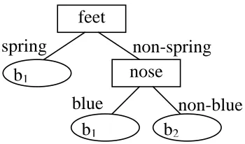
Figure 2.4: A case of the Zoombinis game for a human subject.

Table 2.1: The attribute values of the first three Zoombinis in Figure 2.4 . Zoombini ID hair eyes nose feet

01 small glasses green springs 02 shaggy glasses orange springs 03 shaggy sun glasses red springs

(36)

2.3. MCL-LA 23

01 02 03 09

1

11 04 14 16

12

10

06 08

05 07 13 15

b1:

b2:

Figure 2.5: Zoombinis going through b1 (upper) and b2 (lower).

b

1

feet

nose

b

1

b

2

New Paradigms for Active Learning

Scholarship@Western

Scholarship@Western

New Paradigms for Active Learning

New Paradigms for Active Learning

NEW PARADIGMS FOR ACTIVE LEARNING

(Spine title: New Paradigms for Active Learning)

(Thesis format: Monograph)

by

(Eileen) Ai-Ling Ni

Graduate Program in Computer Science

A thesis submitted in partial fulfillment

of the requirements for the degree of

Doctor of Philosophy

The School of Graduate and Postdoctoral Studies

The University of Western Ontario

London, Ontario, Canada

c

THE UNIVERSITY OF WESTERN ONTARIO

School of Graduate and Postdoctoral Studies

CERTIFICATE OF EXAMINATION

Abstract

Acknowledgements

Contents

List of Figures

List of Tables

List of Appendices

Chapter 1

Introduction

1.1

Machine Learning

1.2

Supervised Learning

1.3

Active Learning

1.3.1

Active Learning Scenarios

1.3.2

Active Learning Query Strategies

1.3.3

Variants of Active Learning

1.3.4

Limitations of Traditional Active Learning Paradigms

1.4

New Paradigms of Active Learning: an Overview

1.4.1

Learning Actively and Conservatively

1.4.2

Learning Actively and Aggressively

1.4.3

Learning Actively with Conservative-Aggressive Tradeo

ff

1.4.4

Learning Actively with Minimal

/

Maximal E

ff

ort

1.5

Contributions of the Thesis

Chapter 2

Learning Actively and Conservatively

2.1

Related Works

2.2

Most-Certain Learning (MCL) Strategy

2.3

MCL-b Learning Algorithm

2.3.1

MCL-b Implementation Details

2.3.2

Application in the Educational Game Zoombinis

b

feet

nose

b

b

spring

non-spring

blue