Reduct Based Rule Generation for Medical Application Using Rough Sets

(1)

Volume 3, No. 5, Sept-Oct 2012

International Journal of Advanced Research in Computer Science

RESEARCH PAPER

Available Online at www.ijarcs.info

ISSN No. 0976-5697

Reduct Based Rule Generation for Medical Application Using Rough Sets

Renu Vashist*, Prof. M.L Garg School of Computer Science Engineering Shri Mata Vaishno and Engineering Shri Mata Vaishno

Devi University, Katra, India

[email protected]

Abstact Rough set theory is an important tool to intelligent data analysis. It is used for dealing with uncertainty in the hidden pattern of data. This paper outlines concepts of the rough set theory for finding decision rules. It assumes that the information about the real world is given in the form of an information table which represents input data, gathered from any domain, such as, medicine, financial markets, banking, etc.. In this study we have acquired the data from the medical science and framed some rules using concept of reduct to make the decision related to the heart problem of a patient. Application of intelligent methods in medical science is a very challenging issue and will be of utmost importance in the future. In this research paper basic ideas of rough set theory are presented with possible intelligent applications for medical case of heart patients.

Keywords Rough Set, Information System, Rule Generation, Reduct, Core, Lower Approximation, Upper Approximation, Decision Algorithm.

I. INTRODUCTION

Rough Set Theory, proposed in 1982 by Zdzislaw Pawlak, is in a state of constant development. Its methodology is concerned with the classification and analysis of imprecise, uncertain or incomplete information and knowledge, and is considered one of the first non-statistical approaches in data analysis [1][2]. The fundamental concept behind Rough Set Theory is the approximation of lower and upper spaces of a set, the approximation of spaces being the formal classification of knowledge regarding the interest domain. The subset generated by lower approximations is characterized by objects that will definitely form part of an interest subset, whereas the upper approximation is characterized by objects that will possibly form part of an interest subset.

Every subset defined through upper and lower approximation is known as Rough Set. Over the years this theory has become a valuable tool in the resolution of various problems, such as representation of uncertain or imprecise knowledge, knowledge analysis, evaluation of quality and availability of information with respect to consistency and reasoning based upon uncertain and reduct of information[7] [10].

II. INFORMATION SYSTEM OR INFORMATION

TABLE

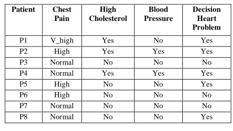
An information system or information table can be viewed as a table, consisting of objects (rows) and attributes (columns). It is used in the representation of data that will be utilized by Rough Set, where each object has a given amount of attributes. These objects are described in accordance with the format of the data table, in which rows are considered objects for analysis and columns as attributes [4] [5][6]. An example of an information system is shown as Table 1.

A. Indiscernibility Relation:

[image:1.612.328.567.416.551.2]

Indiscernibility Relation is a central concept in Rough Set Theory, and is considered as a relation between two objects or more, where all the values are identical in relation to a subset of considered attributes. This relation is an equivalence relation, where all identical objects of set are considered as elementary set [3]. Indiscernibility relation is the basis for set approximation.

Table 1: Information Table

Patient Chest Pain

High Cholesterol

Blood Pressure

Decision Heart Problem

P1 V_high Yes No Yes

P2 High Yes Yes Yes

P3 Normal No No No

P4 Normal Yes Yes Yes

P5 High No No Yes

P6 High No No No

P7 Normal No No No

P8 Normal No No Yes

B. Approximations:

Rough Sets Theory, is more useful to deal with approximations. For each concept X the greatest definable set contained in X and the least definable set containing X are computed. The former set is called a lower approximation of X the latter is called an upper approximation of X. Below is presented and described the types of approximations that are used in Rough Sets Theory[8][10].

a. Lower Approximation:

(2)

b. Upper Approximation:

Upper Approximation is a description of the objects that possibly belong to the subset of interest.

c. Boundary Region:

Elements of the boundary region cannot be decisively classified as members of the set X.

If the boundary region is empty then the set is Crisp. If the boundary region is non empty then the set is rough.

III. DECISION ALGORITHM

Each row of a decision table determines a decision rule, which specifies the decisions (actions) that must be taken when conditions indicated by condition attributes are satisfied. Table 1 shows that both patient5(P5) and patient6(P6) and similarly patient7(P7) and Patient8(P8) suffer from the same symptoms since the condition attributes of Chest Pain, High Cholesterol and Blood Pressure possess identical values, however, the values of decision attribute differ. These set of rules are known as either inconsistent, non-determinant or conflicting. Rules generated by patient1 (P1), patient2(P2) and patient3(P3), patient4(P4) are known as consistent, determinant or non conflicting or simply, a rule.

The number of consistent rules, contained in the decision table are known as a factor of consistency,. Which can be denoted by γ(C, D), where C is the cond ition an d D the decision. If γ(C,D) = 1, the decision table is consistent, but if γ(C,D) ≠ 1 the decision table is inconsistent.

Given that in table 1, γ(C,D) = 4/8 ≠ 1 that is the Table 1 is inconsistent because it possesses four inconsistent rules (for patient5, patient6, patient7 and patient8) and four consistent rules ( for patient1, patient2, patient3, patient4), inside of universe of eight rules [4]. Where γ(C,D) is define as No. of consistent rules divided by Total no. of rules.

The decision rules are frequently shown as implications in the form of “if... then... “.

In table1 we have eight objects. B ={ P1, P2, P3, P4, P5, P6, P7, P8}

Condition attributes of Table 1 are = {Chest Pain, High Cholesterol, Blood Pressure}

Decision attribute of Table 1 = {Heart Problem}

Table 2: Values of All Attributes

Attributes Nominal Values

Condition Attributes

Chest Pain, High Cholesterol, Blood Pressure

High, Normal, V_high Yes, No Yes, No

Decision Attribute

Heart Problem Yes, No

A. Indiscernibility Relations:

In Table1 the attribute Chest Pain generates three Indiscernible relation.

{P1}, {P2, P5, P6}, {P3, P4, P7, P8}

Organize Table1 w.r.t Chest Pain attribute and getting a new table i.e Table 3

Table 3: Indiscernible Relation According To Chest Pain

Decision Heart Problem

P2 High Yes Yes Yes

P5 High No No Yes

P6 High Yes Yes No

P3 Normal No No No

P4 Normal No No Yes

P7 Normal No No No

P8 Normal No No Yes

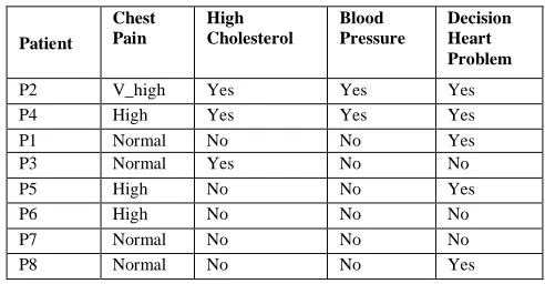
The attribute High Cholesterol generates two Indiscernible relations

{P1, P2, P4}, {P3, P5, P6, P7, P8}

[image:2.612.329.573.297.423.2]

Arranging Table1 according to attribute High Cholesterol and forming a new table i.e Table 4

Table 4: Indiscernible Relation According To High Cholesterol

P2 High Yes Yes Yes

P4 Normal Yes No Yes

P3 Normal No Yes No

P5 High No No Yes

P6 High No No No

P7 Normal No No No

P8 Normal No No Yes

The attribute Blood Pressure generates two indiscernible relation

{P1, P3, P5, P6, P7, P8}, {P2, P4}

[image:2.612.326.572.509.637.2]

Arranging Table I according to attribute Blood Pressure i.e Table5.

Table 5: Indiscernible Relation According To Blood Pressure

Patient

Chest Pain

P2 V_high Yes Yes Yes

P4 High Yes Yes Yes

P1 Normal No No Yes

P3 Normal Yes No No

P5 High No No Yes

P6 High No No No

P7 Normal No No No

P8 Normal No No Yes

The decision attribute generate two indiscernible relation {P1, P2, P4, P5, P8},and {P3, P6, P7}.

B. Lower and Upper Approximations:

(3)

Heart Problem is Yes as per set of objects = {P1, P2, P4, P5, P8}

Heart Problem is No as per set of objects = {P3, P6, P7}

Lower approximation of patient having Heart Problem = {P1, P2, P4, }

Lower approximation of patient not having Heart Problem = {P3}

Upper approximation of patient having Heart Problem = {P1, P2, P4, P5, P6, P7, P8}

Upper approximation of patient not having Heart Problem = {P3,P5, P6, P7, P8}

Boundary region of the patient that does not have Heart Problem = {P5, P6, P7, P8}

Boundary region of the patient that have Heart Problem = {P5,P6, P7, P8}

C. Data Reduction or Reduct:

The form in which data is presented within an information system must guarantee that the redundancy is avoided as it implicates the minimization of the computational complexity in relation to the creation of rules to facilitate the extraction of knowledge [3]. A reduct is a subset of necessary minimum data which provides the original properties of the information or accuracy of information table are maintained. Therefore, the reduct must have the capacity to classify objects, without altering the form of knowledge representation.

D. Removal of Inconsistent Data:

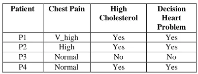
[image:3.612.349.550.428.503.2]

In Table I we have inconsistent data i.e the Table1 is inconsistent or conflicting because for P7 and P8 the values of all condition attributes is the same but the value of decision attribute is different. Similarly for P5 and P6 the values of all condition attributes is the same but the value of decision attribute is different. There is inconsistency in the table. This inconsistency has to remove the so that our information table become consistent or non conflicting. After removing P7, P8 and P5, P6 from Table I we are left with the consistent part of the table. Table 6 represent the consistent part of Table 1.

Table 6:Consistent Part of Table 1

P2 High Yes Yes Yes

P3 Normal No No No

P4 Normal Yes Yes Yes

E. Implementation Technique:

For generating the decision rules using Rough Set Theory there are various methods. But for this paper we generate decision rules using reducts. The rules generated using reducts are more important and significant because reduct is a reduced subset of original set that keeps the consistency of the table. A reduct is a subset of attributes that is jointly sufficient and individually necessary for preserving the same information under consideration as provided by the original set of attributes [1]. Find all possible reduct of Table 6. There are three reduct set that keeps the consistency of the table .

Reduct1 = {Chest Pain, High Cholesterol} Reduct2 = {Chest Pain, Blood Pressure} Reduct3 = { High Cholesterol, Blood Pressure}

Now we define a notion of a core of attributes. Let B be a subset of A. The core of B is a set of all indispensable attributes of B. The following is an important property, connecting the notion of the core and reducts

Core(B) = ∩ Red(B),

Where Red(B) is the set off all reducts of B. Because the core is the intersection of all reducts, it is included in every reduct. The core is the most important subset of attributes, we cannot remove any of core elements without affecting the classification power of attributes. The attribute in core has the maximum significance. Core can be an empty set. In our case there is no element in core, this signifies that we can not easily find which attributes are more important and which are less important. For considering all the attributes of the dataset we will consider all the reduct one by one and eliminate the duplicate rows if any, from all the reduct for reducing the dataset.

Our main aim is to generate the consistent rules from the minimum subset of data that preserves the consistency of original subset. For this removing the duplicate rows from the dataset because they lead to the same decision.

Draw reduct1 which is the reduced sub set of original set that retains the accuracy of original features. We can consider any of the reduct for generating the rules. Finding all the reducts of a decision table is NP-Hard. But for this paper we will consider all the reducts, reduce them one by one and then again combine all the reduced subset by taking the intersection of them.

Table 7: Reduct 1

Patient Chest Pain High

Cholesterol

P1 V_high Yes Yes

P2 High Yes Yes

P3 Normal No No

P4 Normal Yes Yes

[image:3.612.45.278.516.588.2]

Considering Reduct 2 and drawing it in the form of Table.

Table 8: Reduct 2

Patient Chest

Pain

P1 V_high No Yes

P2 High Yes Yes

P3 Normal No No

P4 Normal Yes Yes

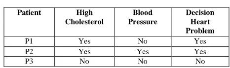
Considering Reduct 3 of Table 6

Table 9: Reduct 3

Patient High

Cholesterol

P1 Yes No Yes

P2 Yes Yes Yes

(4)

P4 Yes Yes Yes

[image:4.612.44.277.148.217.2]

After studying the Table 9 we find that there are two duplicate rows i.e P2 and P4 are duplicate. For P2 and P4 all the condition and decision attribute values are same. We can remove any one of these two rows from Table 9. After the removal of P4 from Table 9 we get Table 10.

Table 10:

Patient High

Cholesterol

P1 Yes No Yes

P2 Yes Yes Yes

P3 No No No

Taking the intersection of Table 7,Table 8 and Table 10 and generating Table 11.

Table 11:

Patient Chest

Pain

P2 High Yes Yes Yes

P3 Normal No No No

Qualitative variables in the above table have been assigned numerical values as follows

X1…..Chest Pain (V_high, 3) ,(High, 2) and (Normal, 1) X2…..High Cholesterol (Yes ,1) and (No, 0)

X3 …..Blood Pressure (Yes ,1) and (No, 0) X4……Heart Problem (Yes ,1) and(No, 0)

Table 12: Decision Table

Patient X1 X2 X3 X4

P1 3 1 0 1

P2 2 1 1 1

P3 1 0 0 0

IV. DECISION RULES

In Table 12 there are some certain rules. Generating certain rules. Rules are represented in the form of, if— then….. Decision rules are implications Φ →Ψ, where Φ and

Ψ are formulas called conditions and decisions of the rule

respectively − built up from elementary formulas (attribute, value) combined together by means of propositional connectives „and”, „or” and „not” in a standard way. Decision rules are prescription of decision (action) that must be made when some condition are satisfied [9]. Here decision is a dependent variable and conditions are independent variables.

Rules generated by Table 12 are followings. These rules are generated by using ROSE2 software.

rule 1. (chest_pain = 1) => (heart_problem = 0); [1, 1, 100.00%, 100.00%] [1, 0] [{3}, {}] rule 2. (cholesterol = 0) => (heart_problem = 0); [1, 1, 100.00%, 100.00%] [1, 0] [{3}, {}] rule 3. (chest_pain = 3) => (heart_problem = 1);

[1, 1, 50.00%, 100.00%] [0, 1] [{}, {1}]

rule 4. (chest_pain = 2) => (heart_problem = 1); [1, 1, 50.00%, 100.00%] [0, 1] [{}, {2}]

rule 5. (cholesterol = 1) => (heart_problem = 1); [2, 2, 100.00%, 100.00%] [0, 2] [{}, {1, 2}] rule6 (blood_pressure = 1) => (heart_problem = 1); [1, 1, 50.00%, 100.00%] [0, 1] [{}, {2}]

V. CONCLUSION

In the last two and a half decades the field of rough data set has taken a gigantic leap in terms of its applications in the growing number of disciplines like, economics, finance, medicine, business management, environmental engineering, software engineering, decision analysis, molecular biology and pharmacy. This paper outlines concepts of the rough set theory for finding decision rules. In this paper we have acquired the data from the medical field and framed some rules to make the decision related to the heart problem of a patient. We aims to generate rules using reducts of decision table because reduct contains all the important attributes of a decision table and hence generates the important and significant rules.

VI. REFERENCES

[1]. Z. Pawlak,. Rough Sets, International Journal of Information and Computer Sciences, Vol. 11, 1982 , pp. 341- 356.

[2]. Z. Pawlak, Rough Sets: Theoretical Aspects of Reasoning about Data., Kluwer Academic Publishers, ISBN 0-79231472, Norwell-USA, 1991.

[3]. Z.Pawlak, J. Grzymala-Busse, R.Slowinski, W. Ziarko, Rough Set,communications of the ACM, Vol. 38, No. 11, Nov. 1995, pp. 88-95, ISSN 0001-0782.

[4]. Z. Pawlak Vagueness - a Rough Set View, In: Lecture Notes in Computer Science- 1261, Mycielski, J; Rozenberg, G. & Salomaa, A. (Ed.), 1997, pp. 106-117, Springer, ISBN 3-540-63246-8, Secaucus-USA.

[5]. Z. Pawlak,. Granularity of Knowledge, Indiscernibility and Rough Sets, The 1998 IEEE International Conference on Fuzzy Systems Proceedings - IEEE World Congress on Computational Intelligence, pp. 106-110, ISBN 0-7803-4863-X, May 4-9, 1998,Anchorage-USA, IEEE Press, New Jersey-USA

[6]. T.Y Lin, An Overview of Rough Set Theory from the Point of View of elational Databases, Bulletin of International Rough Set Society, Vol. 1, No. 1, 1997, pp. 30- 34, ISSN 1346-0013.

[7]. D.J. Hand, H. Mannila, P. Smyth, . Principles of Data Mining. Cambridge, MA: MIT Press, 2001 .

(5)

[9]. R. Agrawal, Fast Discovery of Association Rules, Advances in Knowledge Discovery and Data Mining. 1995, (AAAI/MIT Press, Cambridge, MA)