Volume 3, No. 7, Nov-Dec 2012
International Journal of Advanced Research in Computer Science RESEARCH PAPER
Available Online at www.ijarcs.info
ISSN No. 0976-5697
An efficient segmentation of MRI images using different methods of wavelet transform
Ram Krishna Deshmukh*
Department of ET&T CSVT University
Bhilai, India.
Yogesh S. Bahendwar
Department of ET&T CSVT University
Bhilai, India.
Abstract: Segmentation is the process of separate an observed image into its homogeneous or constituent regions. The goal of segmentation is to simplify or change the representation of an image into something that is more meaningful and easier to analyze. It is important in many computer vision, medical field and image processing application. In computer vision, segmentation refers to the process of partitioning a digital image into multiple regions. Spinal cut MR Images have a number of features, especially the following: Firstly, they are statistically simple; MR Images are theoretically piecewise constant with a small number of classes. Secondly, they have relatively high contrast between different tissues. Additionally, image segmentation has applications separate from computer vision; it is frequently used to aid in isolating or removing specific portions of an image. Image segmentation is typically used to locate objects and boundaries in images. The problem becomes more compound while segmenting noisy images. Segmentation of medical imagery is a challenging task due to the complexity of the images, as well as to the absence of models of the anatomy that fully capture the possible deformations in each structure. Spinal cut tissue is a particularly complex structure, and its segmentation is an important step for derivation of computerized anatomical atlases, as well as pre- and intra-operative guidance for therapeutic intervention. Watershed based image segmentation using wavelet model. Image segmentation, feature extraction and image components classification form a fundamental problem in many application of multi-dimensional signal processing. The paper is devoted to the use of wavelet transform for feature extraction associated with image pixels and their classification in comparison with the watershed transform. A specific attention is paid to the use of Haar, db wavelet or other transform as a tool for image compression and image pixels feature extraction. Proposed algorithm ‘bio’ & different wavelet is verified for simulated images and applied for a selected MR image, using image processing in the MATLAB platform.
Key words: MRIS, IFE & SDF feature extraction, WST, WT & PSNR, MSE. *For future corresponding.
I. INTRODUCTION
The contrast in an MR image depends upon the way the image is acquired. MRI is an advanced medical imaging technique providing rich information about the human soft tissue anatomy. It has several advantages over other imaging techniques enabling it to provide 2-dimensional data with high contrast between soft tissues. However, the amount of data is far too much for manual analysis/interpretation, and this has been one of the biggest obstacles in the effective use of MRI. For this reason, automatic or semi-automatic techniques of computer-aided image analysis are necessary. Segmentation of MR images into different tissue classes, especially gray matter, white matter and cerebrospinal fluid, is an important task. Brain MR Images have a number of features, especially the following: Firstly, they are statistically simple; MR Images are theoretically piecewise constant with a small number of classes. Secondl y, they have relatively high contrast between different tissues. By altering radio frequency and gradient pulses and by carefully choosing relaxation timing, it is possible to highlight different component in the object being imaged and produce high contrast images.[5]
II. WEIGHTING AND DENSITY
MR images can be acquired using different techniques. The resulting images highlight different properties of the depicted materials. The most common weightings are T1 and T2, which highlight the properties T1-relaxation and T2-relaxation respectively. Selection of the most appropriate weighting is important for a successful segmentation [1].
T1-images show high contrast between tissues having
T1-relaxation time emit little signal and thus they will be dark in the resulting image. In T1-images air, bone and CSF have low intensity, gray matter is dark gray, white matter is light gray, and adipose tissue has high intensity. T1-images have high contrast between white matter and gray matter.[1]
In T2-images, white matter and gray matter are gray and have similar intensities. CSF is bright, while bone, air, and fat appear dark. As opposed to T1-images, T2-images have high contrast between CSF and bone. The contrast between white matter and gray matter is not as good as in T1-images.
Spin density or Photon Density (PD) is the most like Computed Tomography (CT) of all the MR contrast parameters. The spin density is simply the number of spins in the sample that can be detected. The observed spin density in medical imaging is always less than the actual spin density due to the fact that many spins are bound and lose signal before they can be observed.
III. MR IMAGE SEGMENTATION
Segmentation of medical imagery is a challenging task due to the complexity of the images, as well as to the absence of models of the anatomy that fully capture the possible deformations in each structure. Brain tissue is a particularly complex structure, and its segmentation is an important step for derivation of computerized anatomical atlases, as well as pre- and intra-operative guidance for therapeutic intervention.
has proven to be important in the evaluation of response to therapy. Other applications of MRI segmentation include the diagnosis of brain trauma where white matter lesions, a signature of traumatic brain injury, may potentially be identified in moderate and possibly mild cases. These methods, in turn, may require correlation of anatomical images with functional metrics to provide sensitive measurements of brain trauma. MRI segmentation methods have also been useful in the diagnostic imaging of multiple sclerosis.
IV. SEGMENTATION PROCESS
Figure. 1 Preprocessing of segmentation
V. WAVELET TRANSFORM
Wavelet transforms have been successfully used in many fusion schemes. A common wavelet analysis technique used for fusion is the discrete wavelet transform (DWT) [2, 3]. It has been found to have some advantages over pyramid schemes such as: increased directional information[2]; no blocking artifacts that often occur in pyramid-fused images [2]; better signal-to-noise ratios than pyramid-based fusion [3]; improved perception over pyramid-based fused images, compared using human analysis [2, 3].
A major problem with the DWT is its shift variant nature caused by sub-sampling which occurs at each level. A small shift in the input signal results in a completely different distribution of energy between DWT coefficients at different scales. A shift invariant DWT (SIDWT), yields a very over-complete signal representation as there is no sub-sampling.
Watershed segmentation is a morphological based method of image segmentation. The gradient magnitude of an image is considered as a topographic surface for the watershed transformation. Watershed lines can be found by different ways. The complete division of the image through watershed transformation relies mostly on a good estimation of image gradients. The result of the watershed transform is degraded by the background noise and produces the over-segmentation. Also, under segmentation is produced by low-contrast edges generate small magnitude gradients, causing distinct regions to be erroneously merged [4].
In order to reduce the deficiencies of watershed, many pre-processing techniques are proposed by the different researcher’s presents a robust watershed segmentation using wavelets where wavelets technique is used to de-noise the image and an efficient watershed algorithm based on connected components.
A proposed method of watershed segmentation using prior shape and appearance knowledge to improve the segmentation results etc. But most of the techniques previously proposed consider the over segmentation problems and focus on the denoising of the image [5]. The image low contrast and under segmentation problem is not yet addressed by most of the researchers.
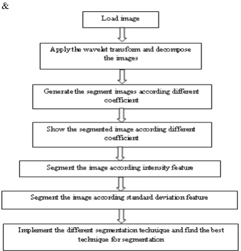
VII. METHODOLOGY
Figure.2 Process of image segmentation based on watershed
&
VIII. RESULT
We segment the different MRI images by wavelet & watershed methods. The result is shown in fig.4 to fig.7 & fig.8 to fig.9. In this paper we apply the two segmentation technique. For these two techniques we segment the different images like our image and MRI images. This is shown in fig.4 to fig.9. The wavelet segmentation is mainly for gray images and its segment, in only for area of interest. In the watershed technique we segment the images on different texture based, the segmentation images are shown in result.
A. Segmented output of Brain MR Image using WAVELET:
Figure.5 (a) original image, (b) detail coefficient, (c & d) Vertical & Horizontal coefficient of image segmentation using wavelet transform.
Figure.5Example image of author (for fig.4)
Figure.6 wavelet result (a) Intensity feature (b) SD feature of image segmentation.
Figure.7 Example image of author (for fig.6)
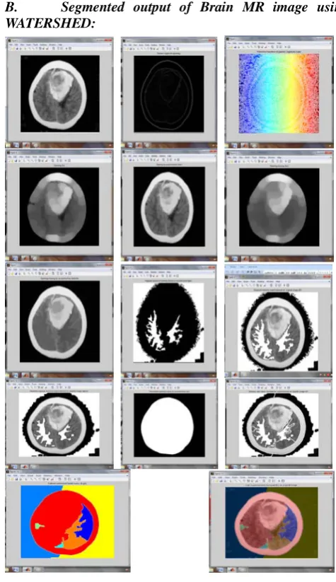
B. Segmented output of Brain MR image using WATERSHED:
Figure. 8 Segmented watershed result (1) to (15) dif. feature.
IX. CONCLUSION
X. ACKNOWLEDGMENT
The authors would like to thank the reviewers for their comments that helped to improve the quality of this paper.
XI. REFERENCE
[1]. D.L. Pham, J. L. Prince, “Adaptive fuzzy segmentation of magnetic resonance images, IEEE Trans. Medical Imaging, vol. 18, 1999.
[2]. H. Li, S. Manjunath, and S. Mitra. Multisensor image fusion using the wavelet transform. Graphical Models and Image Processing, 57(3):235–245, 1995.
[3]. T.Wilson, S. Rogers, and M. Kabrisky. Perceptual based hyperspectral image fusion using multi-spectral analysis. OpticalEngineering, 34(11):3154–3164, 1995.
[4]. P. Scheunders and J. Sijbers. Multiscale watershed segmentation of multivalued images. In International Conference on Pattern Recognition, Quebec, 2002.
[5]. Ram Krishna Deshmukh &Yogesh Bahendwar, International Journal of Advanced Research in Computer Science, 3 (1), Jan –Feb, 2012, 65-69.
[6]. Ram Krishna Deshmukh &Yogesh Bahendwar, "A competent MRI images segmentation using wavelet transform”, International Journal of Computer Science and Management Research,Vol. 1 Issue 5, Dec. 2012.
[7]. Ram Krishna Deshmukh &Yogesh Bahendwar, “MR image segmentation using wavelet and watershed transforms”, International Journal of Societal Application of Computer Science,Vol. 1 Issue 2 Dec. 2012.
[8]. Ram Krishna Deshmukh &Yogesh Bahendwar,“image segmentation with standard deviation feature using wavelet transforms”, International Research Journal of Computer Science Engineering and Applications, Vol. 1 Issue 3 Dec. 2012.
[9]. Ram Krishna Deshmukh, Y. Bahendwar, “Content-Based Image Retrieval Systems -Using 3D Shape Retrieval Methods with Medical Application”, International Journal of Advanced Research in Computer Science, Vol. 3, No. 1, Jan-Feb 2012.
[10]. Ram Krishna, Yogesh Bahendwar, “Content-Based Image Retrieval Systems in Medical Applications – Clinical Benefits and Future Directions”, International Journal of Computer Science and Network Security, Vol. 12, No. 9, Sep. 2011, pp. 113-120.
(a) (b)
Fig.9 Segmented Image(auther) for Watershed Technique. Fig.10 (a & b) Input spinal cut image for wavelet segmentation.
A2. Best PSNR AND MSE Value For spine MRI image:
1. The max. PSNR is 56.596963 the wavelet filter is Haar. 2. The max. PSNR is 56.291178 the wavelet filter is Bior (3.3) 3. The max. PSNR is 56.291178 the wavelet filter is Bior (3.3). 4. The min. MSE is 0.1423590 the wavelet filter is Haar. 5. The min. MSE is 0.1527430 the wavelet filter is Bior.(3.3). 6. The min. MSE is 0.1527430 the wavelet filter is Bior.(3.3) A3. PSNR AND MSE Value For spine MRI image:-
S.
No. wavelets PSNR1 PSNR2 PSNR3 MSE1 MSE2 MSE3
1 Haar 56.5970 55.5810 56.2382 0.1424 0.1799 0.1546
2 Db1 56.5970 55.5810 56.2382 0.1424 0.1799 0.1546
3 Db3 56.5499 55.2346 56.0259 0.1439 0.1948 0.1624
4 Db5 56.5070 54.9377 55.8285 0.1453 0.2086 0.1699
5 Db7 56.3160 54.5307 55.5374 0.1519 0.2291 0.1817
6 Db9 56.2394 54.1944 55.2757 0.1546 0.2475 0.1930
7 Sym2 56.5788 55.4136 56.1517 0.1430 0.1869 0.1577
8 Sym4 56.5041 55.0421 55.9251 0.1454 0.2036 0.1662
9 Sym6 56.3987 54.7020 55.6616 0.1490 0.2202 0.1766
10 Coifc1 56.5279 55.0867 55.9744 0.1446 0.2016 0.1643
11 Coifc3 56.2200 54.1600 55.2693 0.1553 0.2495 0.1933
12 Coifc5 55.9219 53.6018 54.7502 0.1663 0.2837 0.2178
13 Bior1.1 56.5970 55.5810 56.2382 0.1424 0.1799 0.1546
14 Bior1.5 56.2912 56.2912 56.2912 0.1527 0.1527 0.1527
15 Bior2.4 56.5744 55.0300 55.8678 0.1431 0.2042 0.1684
16 Bior2.8 56.4608 54.2755 55.3156 0.1469 0.2430 0.1912
17 Bior3.3 56.5930 55.5978 56.1379 0.1425 0.1792 0.1582
18 Rbior1.1 56.5970 55.5810 56.2382 0.1424 0.1799 0.1546
19 Rbior2.4 56.1245 54.3875 55.4551 0.1587 0.2368 0.1852
20 Rbior3.3 55.5806 54.1930 55.2871 0.1799 0.2476 0.1925
21 Rbior4.4 56.3616 54.6596 55.6385 0.1503 0.2224 0.1775
22 Rbior6.8 56.1665 54.0694 55.1711 0.1572 0.2548 0.1977