Distinctive Data Hiding in Splines using Robust Image Watermarking

Volume 5, No. 2, March 2014 (Special Issue)

International Journal of Advanced Research in Computer Science

RESEARCH PAPER

Available Online at www.ijarcs.info

CONFERENCE PAPER

Distinctive Data Hiding in Splines using Robust Image Watermarking

Allam Mohan

Dept. Of IT,

Shri Vishnu Engg College for Women, Bhimavaram, AP, India, [email protected]

Salina Adinarayana

Dept Of IT,

Shri Vishnu Engg College for Women Bhimavaram,AP,India [email protected]

S.Sreenivasu,

Dept of IT,

Shri Vishnu Engineering College For Women, Bhimavaram,AP,India,

[email protected]

Abstract: This paper presents a robust image watermarking scheme based on a sample spline approach by extracting distinctive invariant features from images that can be used to perform reliable matching between different objects. The features are invariant to basic image transformations like rotation and scaling. The features are highly distinctive, means that every single feature can be correctly matched with high probability against the features of image.

This paper also describes an approach called object recognition by using these features. The recognition can be done by matching individual features to a database of features from known objects using a fast nearest-neighbour algorithm. We use the low frequency components of image blocks for data hiding In our watermarking algorithm, to obtain high robustness. We use four samples of the approximation coefficients of the image blocks to construct a spline curve in the 2-D space. The slopes of this spline curve are employed for watermarking purpose. We embed the watermarking code by constructing a spline curve according to watermarking bits. To get a maximum likelihood decoder, we use the distribution of the slope of the embedding spline curve for Gaussian samples.

Keywords: Image watermarking, Maximum Likelihood detector, Hermite Spline, Bessel interpolator, gain attack, invariant features, scale invariance, Steganography, Image, Stego Image.

I. INTRODUCTION

Digital watermarking embeds information within a digital work as a part of the media. Watermarking techniques falls into three categories of robust, semi fragile and fragile methods according to their specific applications [1]. Robust watermarking mainly serves for identification purposes while the fragile and semi fragile watermarking are usually employed in authentication applications. Since a good watermarking scheme should always be able to deal with some kinds of attacks, studies in the watermarking research area mostly target robust watermarking problems [2].

Image matching is a fundamental aspect of many problems in computer vision, including object or scene

recognition, solving for 3D structure from multiple images. This paper describes image features that have make

properties that make them suitable for matching differing images of an object or scene. The features are invariant to image scaling and rotation, and partially invariant to change in illumination and 3D camera viewpoint. The cost of extracting these features is minimized by taking a cascade filtering approach, in which the more expensive operations are applied only at locations that pass an initial test. The major stages of computation used to generate the set of image features are Scale-space extrema detection, Keypoint localization, Orientation assignment, Keypoint descriptor. This approach has been named the Scale Invariant Feature Transform (SIFT) [3], as it transforms image data into scale-invariant coordinates relative to local features.

An important aspect of this approach is that it gen- erates large numbers of features that densely cover the image over the full range of scales and locations. A typ- ical image of size 500×500 pixels will give rise to about 2000 stable features .The quantity of features is particularly important for object recognition, where the ability to detect small objects in cluttered backgrounds requires that at least 3 features be correctly matched from each object for reliable identification. For image matching and recognition, SIFT features are first extracted from a set of reference images and stored in a database. A new image is matched by indi-vidually comparing each feature from the new image to this previous database and finding candidate matching features based on Euclidean distance of their feature vectors.

CONFERENCE PAPER blocks can be well-modelled by Gaussian distribution [4].

The rest of the paper is organized as follows. In Section II, we describe the model of the system. The watermark embedding and decoding process are introduced in Section III. Section IV analyzes and evaluates the performance of the proposed scheme and Section V concludes the paper.

II. SYSTEM MODELING

In this section, we first describe an approach for object recognition using a set of image features.

A. Scale-space extrema detection:

As described in the introduction, we it detect keypoints using a cascade filtering approach that uses efficient algorithms to identify candidate locations. The first level of keypoint detection is to identify locations and scales that can be repeatedly assigned under differing views of the same object. The Detection of locations that are invariant to scale change of the image can be accomplished by searching for stable features against all possible scales, using a scalling function known as scale space.

It is implemented efficiently by using a difference-of-Gaussian function to identify potential interest points that are invariant to orientation and scale. An efficient approach

to construct the D(x, y, σ) is shown in Fig. 1.

a. Local Extrema Detection:

To detect the local minima andmaxima , each sample point is compared to its eight neighbours in the current image and nine neighbours in the scale above and below (see Fig. 2). It is selected only if it is larger than all of these neighbours or smaller than all of points. The cost of this check is low due to the fact that most sample points will be eliminated following the first few checks.

B. Accurate Keypoint Localization:

At each candidate location, a detailed model is fit to determine location and scale. Keypoints are selected based on measures of their stability. Once a keypoint candidate has been found by comparing a pixel to its neighbours, the next step is to perform a detailed fit to the nearby data for location, scale, and ratio of principal curvatures. This information allows points to be rejected that have low contrast (and are therefore sensitive to noise) or are poorly localized along an edge. The initial implementation of this approach simply located keypoints at the location and scale of the central sample point.

Figure 1: For each octave of scale space, the initial image is repeatedly convolved with Gaussians to produce the set of scale space images shown

on the left.

Figure 2: Maxima and minima of the difference-of-Gaussian images are detected by comparing a pixel (marked with X) to its 26 neighbours in 3×3

regions at the current and adjacent scales (marked with circles).

C. Orientation assignment:

One or more orientations are assigned to each keypoint location based on local image gradient directions. All future operations are performed on image data that has been transformed relative to the assigned orientation, scale, and location for each feature, thereby providing invariance to these transformations.

D. The Local Image keypoint Descriptor:

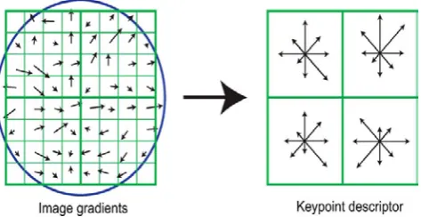
The local image gradients are measured at the selected scale in the region around each keypoint. These are transformed into a representation that allows for significant levels of local shape distortion and change in illumination.

The previous operations have assigned an image location, scale, and orientation to each keypoint. These parameters impose a repeatable local 2D coordinate system in which to describe the local image region, and therefore provide invariance to these parameters. The next step is to compute a descriptor for the local image region that is highly distinctive yet is as invariant as possible to remaining variations, such as change in illumination or 3D viewpoint.

Figure 3: Image gradients and keypoint descriptor

CONFERENCE PAPER computed from an 8 × 8 set of samples, whereas the

experiments in this paper use 4 × 4 descriptors computed from a 16 × 16 sample array.

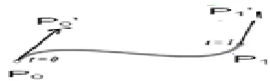
To this aim, we will detect four samples of an independently and identically distributed (i.i.d) Gaussian random variable from the Local Image keypoint Descriptor. We show this host signal as u = [u1, u2, u3, u4] with the Gaussian distribution of N (0, σ2u ). These four samples form two points P1 = [u1, u2] and P2 = [u3, u4] in the 2-D space. We employ Dpk, the slope of the spline at first

control point and Dpk+1

a. Algorithm will generate a cubic curve.

, the slope of the spline at second control point as our watermarking variables. Fig. 4 illustrates these two points as well as the curve derivatives ('slopes') at these points. We can write the procedure as

Figure 4: Hermite Specification Control points P0, P1 and Slopes P0', P1'

Let the parametric curve be P (u) = au3 + bu2 + cu + d. where u is the parameter that ranges from 0 to 1. A Hermite curve has a defined set of coefficients a, b, c, d. Substituting a value u into the equation gives a point on the Hermite curve. Substituting many values of u from 0 to 1 will trace out the curve. Given the two points and two slopes, p0, p1,

p0’ and p1’, our objective is to find the coefficients a, b, c, d.

Derivative of is,

But,

Therefore, in matrix form, =

Solve for a,b,c,d by using matrix inverse:

=

We get:

a = 2 - 2 + + b = -3 + 3 -2 -

Next, Substitute back to equation

We get:

Rearranging.

Now, to embed the M-ary watermark code, we use this equation to generate Hermite spline curve given control points and slopes shown in Fig. 4, depending on the watermark code. In this way, we obtain the watermarked signal.

To extract the hidden bits, an optimum decoder is implemented using M-Hypothesis test as follows. We take the received watermarked signal which consists of the Hermite Spline with two control points and some points on spline curve and calculate the slopes of the Hermite spline curve at each control point. Here the slopes are nothing but the watermarked bits which we have sent it with Host image signal.

In this paper, a new data hiding method has been proposed. The proposed method uses the logical AND operation on the binary value of pixel intensity and binary value of the pixel portion. The message bit is inserted according to the result of logical AND operation. This method makes steganalysis more difficult because it distributes the message uniformly on all the bits of pixel value.

III. PROPOSED METHOD

In this section, we introduce our blind watermarking scheme. As discussed in the previous section, we assume the host signal as a four-sample i.i.d. Gaussian random signal. In practical applications, these four samples can come from approximation coefficients of the image blocks which satisfy our i.i.d. Gaussian assumption according to Kolmogorov Smirnov test results.

Fig. 5 shows a model of watermarking that allows watermark pattern Wa to be dependent on original cover work Co. we can get the final watermarked image Cw from the Watermark embedder. Cwn is the watermarked image with some noise mixing, which we are providing to the Watermark detector. Finally we can get the Watermark as an Output message from detector.

A. Watermark embedding:

We use Hermite cubic interpolation for embedding watermark with the help of four samples as control points and Watermark embedding bits as Slopes at each control point. The interpolator used to construct the curve generally has a parametric representation, i.e. the curve is a two dimensional function of an underlying parameters s,

(1)

Which passes through the collection of sample points {Xi},

(2)

CONFERENCE PAPER This notation allows for easy extension to three

dimensions [5]. The parametric notation also gives an interpolator that is isotropic, i.e. invariant with respect to orientation. The parameter s is usually related to the arc length along the curve. However, using the chord length

Where

With varying linearly between control points, will give equally good results [6]. A further simplification, = i, can be made if the point spacing is fairly uniform.

The interpolation requirement precludes the use of some functions such as quadratic B-splines [7] which are otherwise suitable curve generators. One simple class of functions that both interpolates and can be made sufficiently smooth are the cubic splines and sub-splines. These functions are piecewise cubic, i.e. on any interval ( ) the function is a cubic

+

For sufficient smoothness, we require that the curve be first derivative (C 1) continuous. Such curves are variously known as sub-splines. They are completely defined by the control points { } and the curve derivatives ('slopes') at these points { } (Fig. 6). Each cubic segment can also be represented as a linear combination of four basis or 'blending' [8] functions weighted by the end points and the end-point derivatives

These basis functions, the Hermite Cubic basis functions, are

And are shown in Fig. 6.

Since the sample points { } are given; only the slopes need to be determined in order to specify completely the interpolator. The slope values are the true derivative values of the interpolator , but can only be an estimate of the derivatives of the original curve. The overall Hermite cubic interpolate function is thus composed of piecewise cubic segments h(s) with first-derivative continuity across interval boundaries.

Figure 6. Cubic segment defined by its end points and end-point derivatives

After finding the points on the spline curve, we embed these points in the pixel positions of the spline itself. In our proposed method, we used the logical AND operation on both the selected pixel intensity as well as the selected pixel position. The message bit either will be 0 or 1.The message

bit pixel according to the result of logical AND operation. Firstly, the pixel intensity as well as pixel position is converted into their binary equivalents. Next, the five least Significant bits of each binary equivalent are removed. Now, logical AND operation is applied on these binary equivalents.

The proposed method is shown in fig. 7.

Figure: 7

If we want to insert 0 at a particular position than the results of logical AND operation must be 0, otherwise we make minimum changes to the pixel intensity such that the result of logical AND operation becomes 0. Similarly, if the result of Logical operation is greater than 0 and we want to insert 1 at that position, then it is alright and we don’t need to change the pixel intensity otherwise change intensity of pixel such that result of logical AND operation becomes greater than zero.

B. Insertion Algorithm:

a. Select the first pixel position from the spline. Let the Pixel Position selected is Pi (pos).

b. Find the intensity of selected Pixel Pi. Let intensity of selected pixel Pi is represented by the following equation: -

c. Convert the Pi(intensity) and Pi(pos) into binary values using Binary Converter such that

d. Extract the four Least Significant bits from Bi(intensity)) and Bi(pos) using Bit Extractor such that –

e. Apply the Logical AND operation on the Be i(pos) and Bi (intensity) such that result of logical AND operation i.e. result will be given by the following equation : -

CONFERENCE PAPER f. Now check the message bit mk that we want to

insert in the selected pixel. There are four cases arising over here: -

Case 1: (mk = 0 and Result = 0) then no change in pixel value is required

pixel intensity such that result becomes equal to zero.

Case 3: (mk = 1 and Result > 0) then no change in pixel value is required.

Case 4: (mk = 1 and Result = 0) then change the pixel intensity such that Result becomes greater than zero.

Once the whole data has been inserted, the image is reconstructed from the bit planes. The watermarked image is therefore recomposed With respect to this basic scheme; several modifications have been tested to increase the robustness of the system. Among these, we cite the use of a block-wise embedding scheme in which each block has a different embedding strength value according to some HVS-based features. We are investigating the contrast visibility factor to drive such a scheme.

C. Watermark decoding:

To extract the hidden bits, we need to determine the slope the the Hermite spline by cubic interpolator. To generate the cubic interpolator, the slopes { } must be determined. One common way to specify the slopes is to require second derivative ( ) continuity. The resulting system of tri-diagonal equations can then be solved using various iterative or direct methods [9, 10], with the resulting interpolator being known as the full cubic spline. However, this calculation requires all of the points on the curve to be known, and it is thus not sufficiently local to be used for real-time reconstruction.

D. Extraction Algorithm:

For the extraction algorithm, first five steps are same as in case with insertion algorithm. In the subsequent step, we check the value of Result. If Result is equal to zero then zero is the message bit else 1 is the message bit. Using the same sequence as in the embedding process, the set of selected pixels are extracted and lined up to reconstruct the secret message bits.

We take the received watermarked signal and key for generating the four samples to get two control points. Now we use these points for finding the points on the spline.With these Hermite Spline curve points and control points we can calculate the slopes of the Hermite spline curve at each control point. Here the slopes are nothing but the watermarked bits which we have sent it with Host image signal.

The slopes can also be adjusted interactively. Methods such as Bezier curves [11] have been designed to do this naturally by specifying additional control points. This is not a satisfactory approach if the curve generation is to proceed automatically from a set of sample points without operator intervention. What is required instead is a method to estimate the individual slopes using only a few of the neighbouring points.

The simplest method for determining the slope locally is to use a parabola through a sample point and its left and right neighbours to determine the slope at the point (modifications can be made for the end points of the curve). The parabolic equation

g(s) (

With g ( and g(

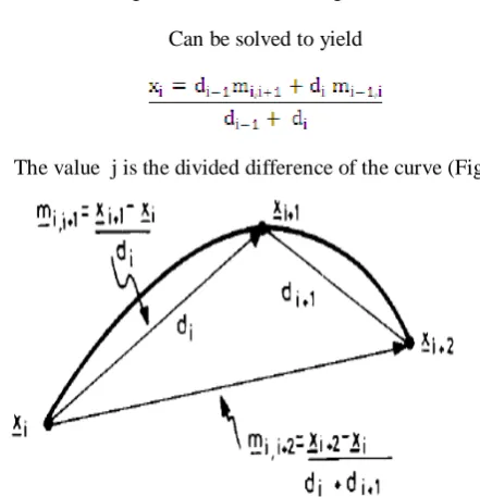
Can be solved to yield

The value j is the divided difference of the curve (Fig. 8),

Figure 8: Divided differences of a curve used to calculate the slopes and are defined as the slope of a line connecting two sample points:

F[ (for short)

The interpolator resulting from this parabolic fit, known as the Bessel interpolator, is quite simple, but does not smooth as well as methods that use more of the neighbouring points. It is, in effect, a four-point interpolator, since the points , , and are needed to define the two end slopes and for the segment .

Higher-order polynomials (such as quadratics) can be fitted to determine the slope, but the exact solution rapidly becomes complex. An assumption of near-uniform spacing can be used to obtain some simple results which take the form of a SUlTI of divided differences weighted by fixed rational numbers (see Appendix ).

IV. EXPERIMENTAL RESULTS

In Fig. 9, we can see the possible Four Basis Functions for Hermite splines.

CONFERENCE PAPER

V. CONCLUSION

In this paper, we presented a novel watermarking approach with the optimal decoder. Watermark embedding is performed by multiplication of M specific matrices to the vector of samples of size four. These matrices construct a Hermite spline curve with the vector of samples and slopes depending on the message symbol. Assuming the host samples to be i.i.d Gaussian, which is often valid for approximation coefficients of image, blocks we obtained a closed form PDF of noisy watermarked samples. Having this distribution function, we designed an optimum ML decoder. We analytically studied and verified the error probability of the proposed decoder in a noisy environment. The proposed algorithm is applied to image signals by using four approximation coefficients of the image blocks which may be selected according to a secret key. In addition to be invariant to the volumetric distortions, several simulations showed that the proposed algorithm is highly robust against common watermarking attacks such as AWGN, compression, and filtering.

VI. APPENDIX

This appendix derives the slope estimate obtained by using a quadratic polynomial fit. An assumption of quasi-uniform spacing is made in order to simplify the solution. The quadratic polynomial

is made to pass through the four neighbouring points

In matrix notation, we have

This general matrix inversion must be performed for each point if a non-uniform grid is assumed. However, if a uniform grid (and hence ) is assumed for the left-hand side, a simplified matrix results

This can be solved for

VII. ACKNOWLEDGMENT

We would like to thank all our colleagues who encouraged and helped in completing this work.

VIII. REFERENCES

[1]. J. Seitz, Digital Watermarking For Digital Media. Arlington, VA, USA: Information Resources Press, 2005.

[2]. Allam Mohan, Salina Adinarayana, “ A New Blind Image Watermarking using Hermite Spline Approach”, (IJCSIT), Vol. 3 (4) , 2012,4812-4817

[3]. David G. Lowe, Distinctive Image Features from Scale-Invariant Keypoints, International Journal of Computer Vision 60(2), 91–110, 2004

[4]. M. A. Akhaee, S. M. E. Sahraeian, B. Sankur, and F. Marvasti, “Robust Scaling-based image watermarking using maximum-likelihood decoder with optimum strength factor,” IEEE Trans. Multimedia,vol.11, no.5,pp.822 –833, Aug. 2009.

[5]. BOEHM, W.: 'On cubics: a survey', ibid., 1982, 19, pp. 201-226

[6]. SZELISKI, R.: 'Real time coding of hand drawn curves', M.Sc. Thesis, University of British Columbia, Vancouver, Canada 1981

[7]. LAPALME, R.S.: "An interactive data reduction technique for line drawings', M.Eng. Thesis, Royal Military College, Kingston, Canada 1977

[8]. DUBE, R.P.: 'Preliminary specification of spline curves', / EEE Trans; 1979, C-28, pp.286-290

[9]. LIOU, M-L.: "Spline fit made easy', / EEE Trans., 1976, C-25, pp. 522- 527

[10]. MOSS, R., and LINGARD, A.: "Parametric spline curves in integer Arithmetic designed for use in microcomputer controlled plotters',Computer. & Graphics, 1979, 4, pp. 51— 6