Nonlinear Observer Design for the Lienard System

(1)

!

"

#"#

$ % %#

&

'

((( )

Nonlinear Observer Design for the Lienard System

Dr. V. Sundarapandian

Professor, Research and Development Centre Vel Tech Dr. RR & Dr. SR Technical University Avadi-Vel Tech Road, Chennai-600 062, INDIA

sundarvtu@gmail.com

Abstract: This paper investigates the nonlinear observer design for the Lienard system. Explicitly, Sundarapandian’s theorem (2002) for observer design for nonlinear systems is used to solve the problem of local exponential observer design for the Lienard system. Lienard system is a classical example in Stability Theory of an asymptotically stable nonlinear system. In this paper, we derive results for exponential observer design for the Lienard system. As a special case, we also construct local exponential observer for the Van der Pol system. Numerical examples and simulations of nonlinear observer design for Lienard system are shown to illustrate the results and validate the proposed observer design for the Lienard system.

Keywords:Lienard System, Van der Pol System, Observer Design, Nonlinear Observers, Exponential Observers, Stability, Nonlinear Systems.

I. INTRODUCTION

In the control systems design, it is often necessary to construct estimates of state variables, which are not available for direct measurement. In such cases, the state vector of the control system can be approximately reconstructed by building an observer which is driven by the available outputs and inputs of the original control system. Local observer design for nonlinear control systems is one of the central problems in the control systems literature.

The problem of designing observers for linear control systems was first introduced by Luenberger ([1], 1966) and that for nonlinear control systems was proposed by Thau ([2], 1973). Over the past three decades, significant attention has been paid in the control systems literature to the construction of observers for nonlinear control systems.

A necessary condition for the existence of an exponential observer for nonlinear control systems was obtained by Xia and Gao ([3], 1988). Explicitly, in [3], Xia and Gao showed that an exponential observer exists for the nonlinear system only if the linearization of the nonlinear system is detectable.

On the other hand, sufficient conditions for nonlinear observers have been obtained in the control systems literature from an impressive variety of points of view. Kou, Elliott and Tarn ([4], 1975) obtained conditions for the existence of exponential observers using Lyapunov-like method. In ([5]-[10]), suitable coordinate transformations were found under which a nonlinear control system is transferred into a canonical form, where the observer design is carried out. In [11], Kazantzis and Kravaris obtained results on nonlinear observer design using Lyapunov auxiliary theorem. In ([12]-[13]), Tsinias derived sufficient Lyapunov-like conditions for the existence of asymptotic observers for nonlinear systems. A harmonic analysis approach was proposed by Celle et al. ([14], 1989) for the synthesis of nonlinear observers.

Necessary and sufficient conditions for the existence of local exponential observers for nonlinear control systems were obtained using differential geometric techniques by

Sundarapandian ([15], 2002). Krener and Kang ([16], 2003) introduced a new method for the design of observers for nonlinear systems using backstepping.

In this paper, we shall use Sundarapandian’s theorem (2002) for observer design for nonlinear systems to solve the problem of designing observers for the undamped oscillator, which is an important model of stable systems in mechanical engineering.

This paper is organized as follows. Section II reviews the definition of nonlinear observers and the results of observability and observers. Section III details the stability result and examples for the Lienard system. Section IV details the design of nonlinear observers for the Lienard system. As a special case, we also consider the nonlinear observer design for the Van der Pol equation. Numerical examples of nonlinear observer design for the Lienard system are also contained in this section. Finally, Section V provides the conclusions of this paper.

II. REVIEW OF OBSERVERS FOR NONLINEAR SYSTEMS

By the concept of a state observer or state estimator for a nonlinear system, it is meant that from the observation of certain states of the system considered as outputs or indicators, it is desired to estimate the state of the whole system as a function of time. Mathematically, observers for nonlinear systems are defined as follows.

Consider the nonlinear system described by

x

=

f x

( )

(1a)

y

=

h x

( )

(1b) where

x

∈

n is the state and

y

∈

p the output. It is assumed that

f

:

n

→

n

,

h

:

n

→

pare 1maps and for some

x

∗

∈

n

,

(2)

Note that the solutions

x

∗ of the equation

( )

0

f x

=

are called the equilibrium points of (1a).

Definition 1. The nonlinear system (1) is called locally observable at the equilibrium

x

∗over a given time interval

[0, ],

T

if there exists

ε

>

0

such that for any two different solutions

x t

( )

and

x t

( )

of the system (1a) with

| ( )

x t

x

∗

|

ε

−

<

and

| ( )

x t

x

∗

|

ε

−

<

for

t

∈

[0, ],

T

the observed functions

h x

and

h x

are different, i.e. there exists some

τ ∈

[0, ]

T

such that

(

h x

)( )

τ

≠

(

h x

)( ).

τ

For the formulation of a sufficient condition for local observability of the nonlinear system (1), consider the linearization of (1) at the equilibrium

x

∗given by

x

=

Ax

(2a)

y

=

Cx

(2b) where

x x

f

A

x

∗

=

∂

=

∂

and _{x x}

.

h

C

x

∗

=

∂

=

∂

Theorem 1. (Lee and Markus, [17], 1971)

If the observability matrix for the linear system (2) given by

1

( , )

n

C

CA

C A

CA

−

=

has rank

n

,

then the nonlinear system (1) is locally observable at

x

∗

.

Definition 2. (Hurwitz Matrices)

An

n n

×

matrix

A

is called Hurwitz if all eigenvalues of

A

have negative real parts.

Next, the definition of nonlinear observers for the given nonlinear system (1) is given. Basically, an observer for a nonlinear system is a state estimator.

Definition 3. (Sundarapandian, [15], 2002) A 1 dynamical system described by

z

=

g z y

( , ),

(

z

∈

n) (3) is a local asymptotic (respectively, exponential) observer for the nonlinear system (1) if the composite system (1) and (3) satisfies the following two requirements:

(i) If

z

(0)

=

x

(0),

then

z t

( )

=

x t

( ),

∀ ≥

t

0.

(ii) There exists a neighbourhood

V

of the equilibrium

x

∗ of n such that for all

z

(0), (0)

x

∈

V

,

the error

e t

( )

=

z t

( )

−

x t

( )

decays asymptotically (resp. , exponentially) to zero.

Theorem 2. (Sundarapandian, [15], 2002)

Suppose that the nonlinear system (1) is Lyapunov stable at the equilibrium

x

∗ and that there exists a matrix

K

such that

A

−

KC

is Hurwitz. Then the dynamical system defined by

z

=

f z

( )

+

K y

[

−

h z

( )

]

(4) is a local exponential observer for the nonlinear system (1). Remark 1. If the estimation error

e

is defined as

e

= −

z

x

,

then the estimation error is governed by the dynamics

e

=

f x

(

+

e

)

−

f x

( )

−

K h x

[

(

+

e

)

−

h x

( )

]

(5)

Linearizing the error dynamics (5) at

x

∗

,

we obtain the linear system

e

=

Ee

,

where

E

=

A KC

−

.

(6) If

( , )

C A

is observable, ie. if the observability matrix

( , )

O C A

has full rank, then the eigenvalues of

E

=

A KC

−

can be arbitrarily assigned in the complex plane. Since the linearization of the error dynamics (5) is governed by the system matrix

E

=

A KC

−

,

it follows that when

( , )

C A

is observable, then a local exponential observer of the form (4) can be always found so that the transient response of the error decays quickly with any desired speed of convergence.

III. STABILITY RESULT AND EXAMPLES FOR THE LIENARD SYSTEM

In this section, we discuss the model and stability result for the Lienard equation [18], which is a classical example of an asymptotically stable system in Mechanical Engineering.

The Lienard equation is described by the second-order differential equation

u

+

α

( )

u u

+

β

( )

u

=

0

(7) where

u

is the displacement of a moving object. Here,

( )

u u

α

is a frictional force that is linear in velocity and

( )

u

β

is the restoring force. Throughout this paper, we shall assume that the functions

α β

,

are continuously differentiable on

−∞ < < ∞

u

and that the functions

α β

,

satisfy the following two assumptions:

α

( )

u

>

0

for

u

≠

0

(8) and that

u

β

( )

u

>

0

for

u

≠

0

(9) For our analysis, it is convenient to express the second-order differential equation (7) as a system of two differential equations. This is carried out by defining the phase variables

1

2

x

u

x

u

=

(10)

Note that (7) is equivalent to the system of differential equations given by

1 2

2

( )

1 2

( )

1

x

α

x x

β

x

=

= −

−

(11)

Next, we state the following result, which is well-known in Lyapunov stability theory [18].

Theorem 3. [18] The Lienard system (11) has an asymptotically stable equilibrium at

x

=

0.

(3)

1

2

1 2 2

0

1

( ,

)

( )

2

x

V x x

=

β τ τ

d

+

x

(12)

We shall establish the asymptotic stability of the equilibrium

x

=

0

by showing that

V

is a Lyapunov function for the system (10).

First, we note that

V

is a positive definite function on

R

2

.

Next, differentiating

V

along the state trajectories of (11), we obtain

V x

( )

= −

α

( )

x x

₁ ₂2

≤

0

(13) which shows that

V

is a negative semi-definite function on

2

.

R

Thus, by Lyapunov stability theory [18], it follows that

0

x

=

is a Lyapunov stable equilibrium of the Lienard system (11).

Next, by LaSalle’s invariance principle [18], we know that the solutions of the Lienard system (11) approach asymptotically the largest invariant set

S

contained in

{

( ,

x x

₁ ₂

)

∈

R

2

: ( ,

V x x

₁ ₂

)

=

0 .

}

Note that

V

=

0

if either

α

( )

x

₁

=

0

or

x

₂

=

0.

By assumption (8),

1

( )

x

0

α

>

if

x

₁

≠

0.

Also, if

x t

₂

( )

=

0,

then

x

₂

=

0,

which implies that

x

₂

= −

α

( )

x x

₁ ₂

−

β

( )

x

₁

=

0.

This yields

β

( ( ))

x t

₁

≡

0

( )

x t

₁

≡

0.

Thus,

V

vanishes only at the trivial solution

x

=

0.

Hence,

S

=

{(0, 0)}.

Thus, by LaSalle’s Invariance Principle, all solutions of the Lienard system (11) approach asymptotically the set

S

or equivalently that the equilibrium

x

=

0

of the Lienard System (11) is asymptotically stable.

Hence, we have shown that the Lienard system (11) is asymptotically stable at the equilibrium

x

=

0.

Example 1. Consider the second-order differential equation described by

u

+

au

+

u

3

=

0

(

a

>

0

) (14) Comparing (14) with the Lienard equation (7), we get

α

( )

u

=

a

and

β

( )

u

=

u

3 (15) Clearly,

α

( )

u

=

a

>

0

and

u

β

( )

u

=

u

4

>

0

for

u

≠

0.

Thus, it is immediate that (14) is indeed a Lienard’s equation. Next, we express this as a system by defining the state variables as

x

₁

=

u

and

x

₂

=

u

.

(16) Hence, we obtain the Lienard system

1 2

3

2 2 1

x

ax

x

=

= −

−

(17)

By Theorem 3, it is immediate that

x

=

0

is an asymptotically stable equilibrium of the system (17).

For numerical simulation, we take

a

=

2.

.

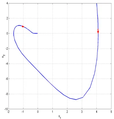
The state orbits of the Lienard equation (16) are depicted in Figure 1.

From Figure 1, it is evident that all the state orbits of the given Lienard’s system (17) approach the equilibrium at

0

[image:3.612.339.536.132.338.2]

x

=

as

t

→ ∞

.

Hence, the Lienard system (17) is asymptotically stable at the equilibrium

x

=

0.

Figure 1. State Orbits of the Lienard System (17)

Example 2 (Van der Pol’s Equation)

Consider the Van der Pol’s equation given by

u

+

ε

(1

−

u u

2

)

+ =

u

0.

(18) Van der Pol’s equation was the fruitful result of the Dutch electrical engineer, Balthazar Van der Pol during the 1920s and 1930s.

Comparing (18) with the Lienard equation (7), we get

α

( )

u

=

ε

(1

−

u

2

)

and

β

( )

u

=

u

(19) Clearly,

α

( )

u

=

ε

(1

−

u

2

)

>

0

for

| | 1

u

<

and

u

β

( )

u

=

u

2

>

0

for

u

≠

0.

Thus, it is immediate that (18) is indeed a Lienard’s equation.

Next, we express this as a differential system by defining the state variables as

x

₁

=

u

and

x

₂

=

u

.

(20) Hence, we obtain the Van der Pol system given by

(

)

1 2

2

2 1

1

1 2

x

ε

x

=

= − −

−

(21)

By Theorem 3, it is immediate that

x

=

0

is an asymptotically stable equilibrium of the system (21).

For numerical simulation, we take

ε

=

2.

.

(4)

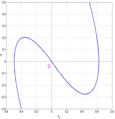
From Figure 2, it is evident that all the state orbits of the given Van der Pol system (21) near the equilibrium

0

x

=

approach the equilibrium as

t

→ ∞

.

[image:4.612.89.289.130.336.2]

Hence, the Van der Pol equation (21) is locally asymptotically stable at the equilibrium

x

=

0.

Figure 2. State Orbits of the Van der Pol’s Equation

III. NONLINEAR OBSERVER DESIGN FOR THE LIENARD EQUATION

In this section, we discuss the nonlinear observer design for the Lienard equation [18], which is a classical example of an asymptotically stable system in Mechanical Engineering.

The Lienard equation is described by the dynamics

1 2

2

( )

1 2

( )

1

x

α

x x

β

x

=

= −

−

(22)

where the functions

α β

,

are continuously differentiable on

u

−∞ < < ∞

and that the functions

α β

,

satisfy the following two assumptions:

α

( )

u

>

0

for

u

≠

0

(23) and that

u

β

( )

u

>

0

for

u

≠

0

(24) Suppose that the displacement

u

is available for measurement, i.e. the output function for the Lienard equation (22) is given by

y

=

x

₁ (25) By Theorem 1, the Lienard equation is asymptotically stable at the equilibrium

x

=

0.

Thus, we can apply Sundarapandian’s theorem (2002) to construct nonlinear observers for the Lienard equation given by (22).

Linearizing the Lienard equation (22) and the output function (25) at

x

=

0,

we obtain the system matrices

A

0

1

,

C

[

1 0

]

r

=

−

∗

where

r

=

β

(0).

Thus, the observability matrix is obtained as

( , )

1 0

0 1

C

C A

CA

=

O

which has full rank.

Thus, by Kalman’s rank condition [19], the pair

( , )

C A

is observable.

Thus, we can always find a gain matrix

K

such that the eigenvalues of the error matrix

E

=

A KC

−

is Hurwitz.

Hence, by Theorem 2 (Sundarapandian, 2002), we obtain the following result.

Theorem 4. A local exponential observer for the Lienard equation (22) is described by the dynamics

1 2

[

₁

]

2

( )

1 2

( )

1

z

K y

z

=

−

α

z z

−

β

z

+

−

(26) where

K

is a gain matrix chosen so that

A

−

KC

is Hurwitz.

Since

( , )

C A

is observable, a gain matrix

K

can be found so that the error matrix

E

=

A

−

KC

has arbitrarily assigned set of eigenvalues with negative real parts.

Example 3. Here, we describe the construction of local exponential observer for the Lienard system described in Example 1 with

a

=

2.

Thus, we consider the nonlinear system

1 2

3

2 2 1

1

2

x

y

x

=

= −

−

=

(27)

The nonlinear system (27) has the linearization pair

0

1

,

[

1 0

]

0

2

A

=

C

=

−

Clearly, the pair

( , )

C A

is observable.

Using the Ackermann formula for the observer gain matrix ([20], p.822), we can choose the gain matrix

K

so that the error matrix

E

=

A KC

−

has the stable eigenvalues

{

− −

4, 4 .

}

A simple calculation using MATLAB yields

6

.

4

K

=

By Theorem 4, a local exponential observer for the Lienard system (27) near the equilibrium

x

=

0

is given by

1 2 ₃

[

₁

]

2 2 1

6

2

4

z

y

z

=

−

z

−

z

+

−

(28) If we define the estimation error as

1 1 1 1 1

2 2 2 2 2

,

e

z

x

z

x

e

z

x

z

x

−

=

−

=

−

then

e t

₁

( )

→

0

and

e t

₂

( )

→

0

exponentially as

t

→ ∞

.

(5)

(0)

2.0

1.5

x

=

and

(0)

0.8

.

1.5

z

=

[image:5.612.91.288.118.301.2]

Figure 3 depicts the exponential convergence of the error trajectories for the observer design of the Lienard system (27).

Figure 3. Observer for the Lienard System (27)

Example 4. Here, we describe the construction of local exponential observer for the Van der Pol system described in Example 2 with

ε

=

2.

Thus, we consider the Van der Pol system given by

(

)

1 2

2

2 1 1 2

1

2 1

x

y

x

=

= − −

−

=

(29)

The Van der Pol system (29) has the linearization pair

0

1

,

[

1 0

]

1

2

A

=

C

=

−

Clearly, the pair

( , )

C A

is observable.

Using the Ackermann formula for the observer gain matrix ([20], p.822), we can choose the gain matrix

K

so that the error matrix

E

=

A KC

−

has the stable eigenvalues

{

− −

2, 2 .

}

A simple calculation using MATLAB yields

2

.

1

K

=

−

By Theorem 4, a local exponential observer for the Van der Pol system (29) near the equilibrium

x

=

0

is given by

(

)

[

]

2 1

1 2

1 1 2

2

2 1

1

z

y

z

=

− −

−

+

−

(30)

If we define the estimation error as

1 1 1 1 1

2 2 2 2 2

,

e

z

x

z

x

e

z

x

z

x

−

=

−

=

−

then

e t

₁

( )

→

0

and

e t

₂

( )

→

0

exponentially as

t

→ ∞

.

For simulation, we take the initial conditions as

(0)

1.0

0.5

x

=

and

(0)

0.6

.

1.0

z

=

Figure 4 depicts the exponential convergence of the error trajectories for the observer design of the system (33).

Figure 4. Observer for the Van der Pol System (29)

IV. CONCLUSIONS

For many real problems of science and engineering, the Lienard system is a classical mechanical system which is asymptotically stable. It has important applications in several stability problems arising in Mechanics and Electrical Engineering. In this paper, we first established a stability result for the Lienard system using the concept of energy function and LaSalle’s Invariance Theorem from the Lyapunov stability theory. Explicitly, we showed that Lienard system has an asymptotically stable equilibrium at the origin. We also deduced the famous Van der Pol system as a special case of the Lienard system. Next, we applied Sundarapandian’s theorem (2002) on nonlinear observer design to construct local exponential observers for the Lienard system. We had also derived local exponential observer for the special case of Van der Pol oscillator. Numerical examples have been worked out in detail for the construction of local exponential observers for the Lienard systems.

V. REFERENCES

[1] D.G. Luenberger, “Observrers for multivariable linear systems”, IEEE Transactions on Automatic Control, AC-2, pp. 190-197, 1966.

[2] F.E. Thau, “Observing the states of nonlinear dynamical systems”, International J. Control, vol. 18, pp. 471-479, 1973.

[3] X.H. Xia and W.B. Gao, “On exponential observers for nonlinear systems”, Systems and Control Letters, vol. 11, pp. 319-325, 1988.

[image:5.612.335.532.154.317.2]

(6)

[5] D. Bestle and M. Zeitz, “Canonical form observer design for nonlinear time-varying systems”, International J. Control, vol. 38, pp. 419-431, 1983.

[6] A.J. Krener and A. Isidori, “Linearization by output injection and nonlinear observers”, Systems and Control Letters, vol. 3, pp. 47-52, 1983.

[7] A.J. Krener and W. Respondek, “Nonlinear observers with linearizable error dynamics”, SIAM J. Control and Optimization, vol. 23, 197-216, 1985.

[8] X.H. Xia and W.B. Gao, “Nonlinear observer design by canonical form”, International J. Control, vol. 47, pp. 1081-1100, 1988.

[9] J.P. Gauthier, H. Hammouri and I. Kupka, “Observers for nonlinear systems”, Proceedings of the 30th IEEE Conference on Decision and Control, vol. 2, pp. 1483-1489, 1991.

[10] J.P. Gauthier, H. Hammouri and S. Othman, “A simple observer for nonlinear systems – Applications to bioreactors”, IEEE Transactions on Automatic Control, vol. 37, pp. 875-880, 1992.

[11] N. Kazantzis and C. Kravaris, “Nonlinear observer design using Lyapunov auxiliary theorem”, Systems and Control Letters, vo. 34, pp. 241-247, 1998.

[12] J. Tsinias, “Observer design for nonlinear systems”, Systems and Control Letters, vol. 13, 135-142, 1989. [13] J. Tsinias, “Further results on the observer design

problem”, Systems and Control Letters, vol. 14, pp. 411-418, 1990.

[14] F. Celle, J.P. Gauthier, D. Kazakos and G. Salle, “Synthesis of nonlinear observers: A harmonic analysis approach”, Math. Systems Theory, vol. 22, pp. 291-322, 1989.

[15] V. Sundarapandian, “Local observer design for nonlinear systems”, Mathematical and Systems Theory, vol. 35, pp. 25-36, 2002.

[16] A.J. Krener and W. Kang, “Locally convergent nonlinear observers”, SIAM J. Control Optimization, vol. 42, pp. 155-177, 2003.

[17] E.B. Lee and L. Markus, Foundations of Optimal Control Theory, New York: Wiley, 1971.

[18] F. Brauer and J.A. Nohel, Qualitative Theory of Differential Equations, New York: Dover Publications, 1969.

[19] I.J. Nagrath and M. Gopal, Control Systems Engineering, 3rd edition, New Delhi: New Age International Ltd., 2002.

[20] K. Ogata, Modern Control Engineering, 3rd edition, New Jersey: Prentice Hall, 1997.

Author:

Dr. V. Sundarapandian is a Research Professor (Systems and Control Engineering) in the Research and Development Centre, Vel Tech Dr. RR & Dr. SR Technical University, Avadi, Chennai since September 2009. Previously, he was a Professor and Academic Convenor at the Indian Institute of Information Technology and Management-Kerala, Trivandrum. He earned his Doctor of Science Degree from the Department of Electrical and Systems Engineering, Washington University, St. Louis, Missouri, USA in May 1996. He has published over 90 research papers in refereed International Journals and presented over 100 research papers in National and International Conferences in India and abroad. He is an Associate Editor of the International Journal on Control Theory and Applications and is in the Editorial Boards of the Journals – Scientific Research and Essays,