The Study of a Flame Propagation in a Rectangular Duct with a Locally Stratified Flow-Field

(1)

University of Windsor University of Windsor

Scholarship at UWindsor

Electronic Theses and Dissertations Theses, Dissertations, and Major Papers

2016

The Study of a Flame Propagation in a Rectangular Duct with a

Locally Stratified Flow-Field

Indika Gallage University of Windsor

Follow this and additional works at: https://scholar.uwindsor.ca/etd

Recommended Citation Recommended Citation

Gallage, Indika, "The Study of a Flame Propagation in a Rectangular Duct with a Locally Stratified Flow-Field" (2016). Electronic Theses and Dissertations. 5906.

https://scholar.uwindsor.ca/etd/5906

This online database contains the full-text of PhD dissertations and Masters’ theses of University of Windsor students from 1954 forward. These documents are made available for personal study and research purposes only, in accordance with the Canadian Copyright Act and the Creative Commons license—CC BY-NC-ND (Attribution, Non-Commercial, No Derivative Works). Under this license, works must always be attributed to the copyright holder (original author), cannot be used for any commercial purposes, and may not be altered. Any other use would require the permission of the copyright holder. Students may inquire about withdrawing their dissertation and/or thesis from this database. For additional inquiries, please contact the repository administrator via email

(2)

The Study of a Flame Propagation in a Rectangular Duct with a Locally Stratified

Flow-Field

By

Indika Gallage

A Thesis

Submitted to the Faculty of Graduate Studies

Through the Department of Mechanical, Automotive and Materials Engineering

In Partial Fulfillment of the Requirements for the Degree of Master of Applied Science at

the University of Windsor

Windsor, Ontario, Canada

2016

(3)

The Study of a Flame Propagation in a Rectangular Duct with a Locally Stratified

Flow-Field

by

Indika Gallage

APPROVED BY:

______________________________________________

Dr. Randy Bowers

Department of Mechanical, Automotive and Materials Engineering

______________________________________________

Dr. Vesselina Roussinova

______________________________________________

Dr. Andrzej Sobiesiak, Advisor

(4)

iii

DECLARATION OF CO AUTHORSHIP AND PREVIOUS PUBLICATIONS

I. Co- Authorship Declaration

I hereby declare that this thesis incorporates material that is result of joint research, as follows: This thesis also incorporates the outcome of a joint research undertaken in collaboration with Zakaria Movahedi, Xisheng Zhao and Dale Haggith under the supervision of professor Andrzedj Sobiesiak. The collaboration is covered in Chapters 4, 5, 6 and 7 of the thesis. In all cases, the key ideas, primary contributions, experimental designs, data analysis and interpretations, were performed by the author, and the contribution of co-authors was primarily through the provision of reviewing the material and by providing advice on improving the ideas to be conveyed.

I am aware of the University of Windsor Senate Policy on Authorship and I certify that I have properly acknowledged the contribution of other researchers to my thesis, and have obtained written permission from each of the co-author(s) to include the above material(s) in my thesis.

I certify that, with the above qualification, this thesis, and the research to which it refers, is the product of my own work.

II. Declaration of Previous Publications

This thesis includes three original conference papers that have been previously published in conference proceedings

Thesis Chapter Publication title/full citation Publication

status*

Chapter 4,5&7 Gallage I, Mohavadi Z, Zhao X, Haggith D., Sobiesiak

A. Investigation of the premixed flame propagation

across the varied Composition Field on a Rectangular

Duct. Proceedings Combustion Institute Canadian

Secretion, University of Windsor, Ontario, Canada:

2014

Published and

presented

-Conference Paper

Chapter 4,5&7 Gallage I, Sobiesiak A, Mohavadi Z. Flame

Propagation in a Rectangular Duct Filled with Stratified Air and Fuel Mixtures. Proceedings Combustion Institute Canadian Section, University of Saskatchewan, SK, Canada: 2015

Published and

presented

(5)

iv Chapter

4,5,6&7

Gallage I, Mohavedi Z, Sobiesiak A. The effect of stratification on the 1st inversion of a Premixed Flame Propagating in a Rectangular Duct. Proceedings Combustion Institute Canadian Section., University of Waterloo, ON, Canada: 2016.

Published and

presented

-Conference Paper

I certify that I have obtained a written permission from the copyright owners to include the above-published materials in my thesis. I certify that the above material describes work completed during my registration as a graduate student at the University of Windsor.

I declare that, to the best of my knowledge, my thesis does not infringe upon anyone’s copyright nor violate any proprietary rights and that any ideas, techniques, quotations, or any other material from the work of other people included in my thesis, published or otherwise, are fully acknowledged in accordance with the standard referencing practices. Furthermore, to the extent that I have included copyrighted material that surpasses the bounds of fair dealing within the meaning of the Canada Copyright Act, I certify that I have obtained a written permission from the copyright owners to include such materials in my thesis.

(6)

v ABSTRACT

This work reports on an experimental investigation of a flame propagating through a propane-air mixture in a rectangular duct where the ignition end is kept shut. Flame propagation through a homogeneous charge with equivalence ratios 0.8, 0.9, 1.0 and 1.1 was investigated initially. The flames were tested with the exit end fully open and fully closed. In all the cases, propagation of the flame occurs through a series of acceleration and deceleration periods. This movement was termed the “Leap Frog” phenomenon. The flame develops a shape called the “tulip flame” at the first period and “flame inversions” during the subsequent periods. The formation of the tulip flame and inversions occur right after the acceleration period in a sequence, suggesting that the Leap Frog phenomenon is influenced by the Rayleigh–Tayler (R-T) instability. Flame images of the tulip flame occurrence are qualitatively similar to the interface evolution of two fluids during the R-T instability. The pressure variation at the ignition end of the duct correlates well with the tulip and inversion formations; with a peak pressure at the inversions and tulip flame formation positions. The pressure was filtered with a low pass filter of 25Hz. This frequency is less than the first harmonic of the longitudinal acoustic frequency of the duct, suggesting that acoustic pressure oscillations do not heavily influence the Leap Frog phenomenon.

(7)

vi

DEDICATION

This MASc thesis

is dedicated

to the people who share their valuable knowledge

(8)

vii

ACKNOWLEDGEMENTS

My Advisor, Dr. Andrzej Sobiesiak is acknowledged with great gratitude for the excellent

atmosphere created which made me enjoy the work rather than do the work. The continuous

supervision and help, whenever needed, was way above expectation. His excellent

understanding and the extraordinary teaching skills made it very easy to tackle problems

always the easy way. He used delicate methods constantly to preserve and polish my own

work.

Dr. Randy Bowers and Dr. Vesselina Roussinova are acknowledged with gratitude for

accepting to be on my committee, for the valuable inputs and being vigilant on my progress

despite their busy schedules.

Dr. Garry Rankin, Dr. David Ting, Dr. Zhou Bao and Dr. Ming Zing are acknowledged

with gratitude for the valuable and very interesting lectures offered to broaden my

knowledge on the study during the course.

My fellow graduate students Xisheng Zhao, Zakaria Mohavedi, Dr. Iain Cameron, Tuan

Nguyen and Dale Haggith for helping me to blend into the culture of the University of

Windsor, for all the fun time and the many valuable inputs for my study.

I admire the high skills of Andy Jenner, Bruce Durfy and Patrick Seguin whom without, I

couldn’t have completed the experimental setup to a very high standard.

The financial support from the Natural Science and Engineering Research Council and the

University of Windsor is gratefully acknowledged.

I would like to thank my friends Chandana and Shiromi Walgama for helping me to settle

in Windsor and for persuading me to register for the MASc at the University of Windsor.

My parents, brother Chanaka and sister Hasini for always offering a shoulder to bear the

strength and being with me on my smiles and tears and for cheering me up whenever things

got complicated in my life.

To my loving wife Rasika, for creating an excellent atmosphere at home to set my mind

free to carry on with the work full time in a peaceful mind and for understanding me

unconditionally and for the valuable ideas and thoughts.

Last but not least my son Sakkya for encouraging me always to stick to my studies which

brought back the joy of learning and Jithara for being my little daughter who refreshes my

(9)

viii

TABLE OF CONTENTS

DECLARATION OF CO AUTHORSHIP AND PREVIOUS PUBLICATIONS ... iii

ABSTRACT ... v

DEDICATION ... vi

ACKNOWLEDGEMENTS ... vii

LIST OF FIGURES ... xiii

LIST OF TABLES ... xvii

LIST OF ABBREVIATIONS ... xix

NOMENCLATURE ... xx

CHAPTER 1 ... 1

1. INTRODUCTION ... 1

1.1. MOTIVATION ... 1

1.2. OBJECTIVE ... 1

1.3. STRATEGY ... 1

CHAPTER 2 ... 3

2. ON LAMINAR AND TURBULENT FLAMES ... 3

2.1. REACTING FLOWS ... 3

2.2. LAMINAR AND PREMIX FLAMES ... 3

2.2.1. Analytical Study of a Laminar Premixed flame ... 4

2.3. TURBULENT PREMIXED FLAMES ... 9

2.3.1. Fluctuation of properties and turbulent intensity ... 10

2.3.2. The relationship of the Reynolds number, Damköhler Number and Karlovitz Number, with length and time scales of turbulent combustion... 10

2.3.3. The Relationship of strain with length and time scales of combustion[7] ... 11

2.3.4. Understanding Premixed Turbulent Flames using Different Regimens ... 12

2.4. RELEVANT HYDRODYNAMIC INSTABILITIES ... 15

2.4.1. Darius–Landau instability ... 15

2.4.2. Rayleigh–Taylor instability ... 16

2.4.3. Richtmyer-Meshkov Instability ... 17

2.5. THE GLOBAL REACTION OF PROPANE WITH AIR AND STOICHIOMETRY ... 18

(10)

ix

2.5.2. Stoichiometry and air to fuel ratio ... 18

2.5.3. The equivalence ratio (Φ) of a combustible mixture ... 19

2.6. DOLTON’S LAW OF PARTIAL PRESSURE AND PREPARATION OF GAS MIXTURES ... 19

2.6.1. Dalton’s Law of Partial Pressure ... 19

2.6.2. Preparation of an air –fuel mixture of a required equivalence ratio ... 20

CHAPTER 3 ... 21

3. BACKGROUND OF FLAME PROPAGATION STUDIES ... 21

3.1. EARLY INVESTIGATIONS OF FLAME PROPAGATION INSIDE DUCTS USING PIONEERING IMAGING TECHNIQUES. ... 21

3.2. INVESTIGATION OF HYDRODYNAMIC INSTABILITIES IN FLAME PROPAGATION THROUGH DUCTS AND THE USE OF FLASH SCHIEREN PHOTOGRAPHY ... 23

3.3. RECENT NUMERICAL AND EXPERIMENTAL INVESTIGATIONS OF PREMIXED FLAME PROPAGATION IN DUCTS ... 24

3.4. STUDIES OF FLAME PROPAGATION THROUGH STRATIFIED MIXTURES ... 28

CHAPTER 4 ... 29

4. EXPERIMENTATION ... 29

4.1. EXPERIMENTAL SETUP... 29

4.1.1. Flame Propagation Duct (FPD) ... 29

4.1.2. Ignition System ... 30

4.1.3. Injection system and injection timing control ... 31

4.1.4. Modifications to the injection system ... 31

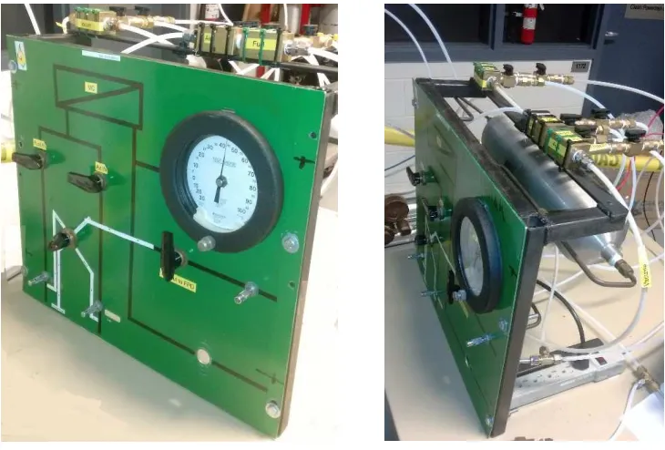
4.1.5. Gas-Mixing Panel and handling of the gas between the gas- mixing panel and flame propagation duct ... 31

4.1.6. The LabVIEW Program ... 33

4.2. UNCERTAINTY ANALYSIS ... 34

4.2.1. Uncertainty of the mass of substance injected ... 34

4.2.2. Uncertainty of the pressure measurement ... 36

4.2.3. Uncertainty of the equivalence ratio ... 38

4.2.4. Uncertainty of distance measurements ... 39

4.2.5. Uncertainty of velocity calculations ... 40

4.2.6. Summary of uncertainties and special points to note ... 43

(11)

x

4.3.1. Data acquisition frequency ... 43

4.3.2. Control program for data DAQ System ... 45

4.3.3. Image Data Acquisition ... 45

4.3.4. Pressure Data Acquisition ... 46

4.3.5. Flow Data Acquisition ... 47

4.4. PROCESSING OF COLLECTED DATA ... 49

4.4.1. Processing of Image Data ... 49

4.4.2. Processing of pressure data ... 51

4.4.3. Processing of Flow Data ... 53

4.5. EXPERIMENTAL PROCEDURES ... 56

4.5.1. Preparation of the air/propane premix at desired equivalence ratio ... 56

4.5.2. Preparation of the duct and other equipment for an experiment ... 57

4.5.3. Identification codes of the experiments ... 58

4.6. STRATEGY FOR EXPERIMENTS AND THE EXPERIMENTAL MATRIX .... 59

4.6.1. Reference trials with a homogeneous mixture ... 59

4.6.2. Fuel injections ... 59

4.6.3. Air injections ... 59

4.6.4. Air-fuel mixture injections... 60

4.6.5. Experimental Matrix ... 61

CHAPTER 5 ... 62

5. RESULTS AND DISCUSSION ... 62

5.1. FLAME PROPAGATION THROUGH THE DUCT WITH HOMOGENEOUS MIXTURES OF Φ=1.1, 1.0, 0.9 AND 0,8 –OPENED AND CLOSED EXIT END ... 62

5.1.1. Introduction ... 62

5.1.2. Correlation between experiments at the same condition to evaluate repeatability . 62 5.1.3. Overview of trials and repeatability ... 63

5.1.4. The absolute flame velocity diagram ... 64

5.1.5. Presentation of initial data ... 65

5.1.6. Common propagation patterns of open end cases, the tulip flame and inversions . 65 5.1.7. Comparison of open-ended cases ... 65

5.1.8. Comparison of closed-end cases ... 69

5.1.9. The analysis of the tulip flame and inversions in open-end and close-end flame propagation ... 71

(12)

xi

5.2. FLAME PROPAGATION THROUGH THE DUCT WITH INJECTIONS ... 77

5.2.1. Injection process analysis ... 77

5.2.2. The variation of injection timing ... 77

5.2.3. Impact of injections ... 78

5.3. VARYING THE MASS OF FUEL INJECTED TO DETERMINE THE CRITICAL MASS OF FUEL TO TERMINATE THE FLAME ... 80

5.3.2. Results and discussion ... 81

5.4. VARYING THE TIME BETWEEN IGNITION AND FUEL INJECTIONS WHEN LESS THAN THE CRITICAL MASS IS INJECTED ... 83

5.5. VARYING THE MASS OF AIR INJECTED TO DETERMINE THE CRITICAL MASS OF AIR TO DISPLACE THE TULIP FLAME. ... 88

5.5.2. Results and Discussion ... 88

5.6. VARYING THE TIME BETWEEN IGNITION AND AIR INJECTIONS WHEN LESS THAN THE CRITICAL MASS IS INJECTED. ... 90

5.7. MIXTURE INJECTIONS... 94

CHAPTER 6 ... 97

6. SUMMARY OF RESULTS ... 97

CHAPTER 7 ... 100

7. UNIQUENESS OF THE STUDY, FINDINGS, CONCLUSIONS AND RECOMMENDATIONS ... 100

7.1. UNIQUENESS OF THE STUDY ... 100

7.2. THESIS FINDINGS ... 100

7.3. CONCLUSIONS ... 101

7.4. RECOMMENDATIONS ... 103

REFERENCES ... 104

(13)

xii

Appendix - A Copyright permission for figures from outside sources used in the thesis ... 109

Appendix - B Governing equations and numerical study for reacting flows ... 111

Appendix - C Uncertainty Analysis ... 115

Appendix - D Design stage uncertainties of equipment used ... 118

Appendix - E Lists of experiments and summaries of experimental results ... 121

(14)

xiii

LIST OF FIGURES

Fig. 1: Image of the flame propagation duct ... 2

Fig. 2: Laminar and turbulent flame shapes during the propagation of the flame ... 3

Fig. 3: Structure of laminar plane premixed flames; modified image published in [7] ... 4

Fig. 4: Flame speed relationships ... 6

Fig. 5: Laminar burning speeds of propane /air at 300 k and 1 bar ... 8

Fig. 6: Turbulent premixed combustion regimes modified diagram using modified image published in [8] ... 13

Fig. 7: Turbulent combustion regimes as a function of non-dimensional numbers; image published in [9] ... 14

Fig. 8: Using the regime diagram to interpret operating ranges of devices; modified image published in [9] ... 14

Fig. 9: Deviation of flow lines leading to Darius-Landau instability; image published in [19] .... 15

Fig. 10: Simulated results of the Rayleigh–Taylor instability; image published in [24] ... 16

Fig. 11: Instability of a plane contact discontinuity from RT Instability image created based on [25] ... 16

Fig. 12: Coexistence of all morphologies- Richtmyer-Meshkov Instability: image published in [29] ... 17

Fig. 13: High speed images of a propagating wave in a closed duct by Ellis in 1928: image published in [37] ... 23

Fig. 14: Initial stages of the shock wave flame and front interaction with three images showing the stages of the development of the tulip flame: image published in [39] ... 23

Fig. 15: The tulip shaped flame captured by Salamandra et al.: Image published in [6] ... 24

Fig. 16: Simplified geometric model of flame front at times between t Sphere and t Wall: image published in [43] ... 25

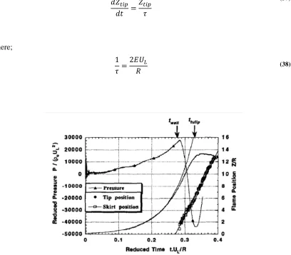
Fig. 17: Normalized superposition plot of pressure at closed end, the position of center of flame tip and of tailing edge of flame skirt; as a function of time. The best fit exponential is also shown: image published in [43] ... 26

Fig. 18: Location of the tulip flame and first inversion in an L shaped rectangular duct; modified image published in [48] ... 27

Fig. 19: Image of the flame propagation duct ... 29

Fig. 20: Schematic diagram of the flame propagation duct ... 29

Fig. 21: Gas mixing panel front ... 32

(15)

xiv

Fig. 23: Piping and instrumentation diagram for the modified mixture panel, connections to the

flame propagation duct and Injectors ... 33

Fig. 24: Calibration chart from Alicat flow meter ... 34

Fig. 25: Experimental setup with the data acquisition and control system. ... 44

Fig. 26: The LabVIEW program to control ignition and DAQ system ... 45

Fig. 27: LabVIEW DAQ Assistant - calibration for pressure recording ... 47

Fig. 28: Block diagram indicating the integral function and filtering used to process the flow data ... 48

Fig. 29: Calibration of the DAQ Assistant for flow meter ... 48

Fig. 30: Using image processing to derive the flame position ... 49

Fig. 31: The Ashcroft pressure gauge dial ... 56

Fig. 32: The AFV Vs Distance diagram ... 64

Fig. 33: Image sequence of the tulip flame and the 1st inversion ... 65

Fig. 34: AFV vs distance for Φ=0.8, exit end opened; experiment #3 ... 66

Fig. 38: Position of the tulip flame for open end flame propagation ... 67

Fig. 39: Comparison of pressure and distance vs time with different equivalence ratios for open exit end ... 68

Fig. 40: Comparison of AFV along the duct with varying initial equivalence ratios for open exit end ... 68

Fig. 41: AFV vs distance Φ=0.8, exit end closed: experiment #23 ... 69

Fig. 42: AFV vs distance Φ=09, exit end closed; experiment #6 ... 69

Fig. 43: AFV vs distance Φ=1.0, exit end opened; experiment #60 ... 69

Fig. 44: AFV vs distance Φ=1.1, exit end closed; experiment #33 ... 69

Fig. 45: Comparison of pressure and distance vs time with different equivalence ratios for closed exit end cases ... 70

Fig. 46: The AFV Vs distance for Ф = 0.8, 0.9, 1.0, and 1.1 for closed exit end ... 71

Fig. 47: Tulip and first inversion for Φ=1.1, open -end and close – end trials ... 72

Fig. 48: Flame front existing between side walls ... 72

Fig. 49 : Acceleration and deceleration during tulip formation in an open-end case ... 74

(16)

xv

Fig. 51: The shape of the flame front corresponding to the velocity fluctuation along the duct for

the tulip formation ... 75

Fig. 52: Formation of the "Tulip Flame" (the time lapsed from the start of ignition is shown) .... 76

Fig. 53: Instantaneous flow Vs time for a single injection ... 77

Fig. 54: Ten instantaneous injections with the same delay and pulse settings... 78

Fig. 55: Image of the injection site 23.5ms after ignition; injection starts when the flame front is 75mm ahead of the injector and continues injecting in trial #311 ... 79

Fig. 56: The details of injection for experiment number 311 ... 79

Fig. 57: Calculated Φ within the duct volume at different distances from the point of injection .. 80

Fig. 58: AFV vs distance diagram for the cases with flame terminations for delayed fuel injections ... 81

Fig. 59: The variation of total distance travelled by the flame before extinction for varied mass of fuel injected to the duct (Trial number shown in figure) ... 81

Fig. 60: Injection and the distance of the flame front variation Vs time, for experiment 273 ... 82

Fig. 61: Schematic diagram of the flame termination of experiment 273 ... 83

Fig. 62: Flame propagation profiles for varied delayed injections of 26.9 mg fuel ... 84

Fig. 63: Flame propagation profiles for varied advanced injections of 27 mg fuel ... 84

Fig. 64: Position of the first inversion vs the absolute flame velocity at 950 mm from the ignition end ... 85

Fig. 65: Position of the first inversion for varied delayed fuel injections ... 85

Fig. 66: Position of the first inversion for varied advanced fuel injections of 27 mg ... 86

Fig. 67: Time Vs velocity diagram for #283 for a fuel injection with a very small delay (0.6ms) 86 Fig. 68: Time Vs velocity diagram for #288 for a fuel injection with a very small advance (4.4ms) ... 86

Fig. 69: Injection and flame propagation pattern for a 14.2 ms advanced fuel injection for trial #302 ... 87

Fig. 70: Injection and flame propagation pattern for a 34.9 ms advanced fuel injection for trial #294 ... 87

Fig. 71: Propagation profiles for air injections over 34.6 mg ... 88

Fig. 72: Propagation profiles for air injections less then 34.6 mg ... 89

Fig. 73: Variation of the position of the tulip with position of the flame at the time of starting air injections ... 89

(17)

xvi

Fig. 75: Injection profile and distance of flame from the ignition end for 65mg of air injected when

the fame front was at 173mm from the ignition end in trial # 337 ... 90

Fig. 76: Comparison of AFV for delayed and advanced air injections below 5 ms ... 91

Fig. 77: Comparison of AFV for delayed and advanced air injections 5ms -40ms ... 91

Fig. 78: Comparison of AFV for delayed and advanced air injections more than 40ms ... 92

Fig. 79: Position of the first inversion for air injections below the critical mass ... 92

Fig. 80: The average AFV Vs delay between air injection and ignition ... 93

Fig. 81: Average AFV for different advanced and delayed fuels injections ... 94

Fig. 82: Flame propagation profiles for mixture injections with no displacement of the tulip flame ... 94

Fig. 83: Mixture injections with displacement of the tulip position ... 95

Fig. 84: Location of the tulip position Vs mass of mixture injected ... 95

Fig. 85: Location of the tulip position Vs the position of the flame at the start of mixture injection ... 96

Fig. 86: Severe perturbations to the flame front by air fuel and mixture injections ... 97

Fig. 87: Flame propagation profiles for injections with less than the critical mass of fuel injections ... 98

Fig. 88: Flame propagation profiles for injections with less than the critical mass of air injections ... 98

Fig. 89: Severe perturbation to the flame front by a fuel injection ... 98

(18)

xvii

LIST OF TABLES

Table 1: Simple classification of flame speeds. ... 6

Table 2: Values for equation (17) plotted in graph in Fig. 5 [12] ... 8

Table 3: Effects of pressure and preheat for laminar flame speed for equation (10)[12] ... 9

Table 4: Data used for calibrating the DAQ Assistant in LabVIEW ... 34

Table 5: Uncertainty of individual parameters to calculate uncertainty of the calibration coefficient for the Alicat flow meter (to be used in the NI DAQ Assistant in LabVIEW) ... 35

Table 6: Uncertainty of individual parameters to calculate the uncertainty of mass of substance injected ... 36

Table 7: The uncertainty values of individual parameters to be used to determine the error in the amplification of the pressure signal ... 37

Table 8: The uncertainty of the equivalence ratio prepared ... 39

Table 9: Uncertainty values for individual parameters to calculate the uncertainty in image processing for distance and velocity for the camera settings to capture the total duct length ... 39

Table 10: Uncertainty values for individual parameters to calculate the uncertainty of velocities calculated from images ... 40

Table 11: Uncertainties for distance and velocity calculated from images for different image calibrations and different velocity calculation methods... 42

Table 12: Summary of uncertainties ... 43

Table 13: General description and settings of the CCD image capturing ... 46

Table 14: Characteristics of the Pressure sensor used ... 46

Table 15: Line tracking data ... 50

Table 16: Time distance and corresponding instantaneous flame velocity table ... 51

Table 17: Values to find the speed of sound ... 52

Table 18: The resonant frequencies of oscillation of the FPD ... 53

Table 19: Values to calculate viscosity of mixture ... 54

Table 20: Results of equations (64),(65) and (66) to find the dynamic viscosity of propane-air mixture @ Ф=1.1 ... 55

(19)

xviii

Table 22: Calculated values for partial pressure and corresponding readings of the instrument used

... 57

Table 23: Procedure to prepare a mixture of propane-air of an equivalence ratio of 1.1 ... 57

Table 24: Description of the flame code ... 59

Table 25: Experimental matrix ... 61

Table 26: Average correlation coefficient calculation ... 62

Table 27: Ascending order of the average correlation coefficients ... 63

Table 28: Statistical analysis of the variation of the starting time of injections for the same settings ... 78

Table 29: Total number of equations to solve a reacting flow problem ... 111

Table 30: Source groups of error represented by the i value ... 117

Table 31: Design errors of Ashcroft type 108 pressure gauge [69] ... 118

Table 32: Design errors of Alicat scientific flow meter [57] ... 118

Table 33: Design errors of NI 6036 DAQ card for 5V range [70] ... 119

Table 34: Design errors of NI 6036 DAQ card for 10V range[70] ... 119

Table 35: Design errors of Kistler 6117BF pressure transducer[59] ... 119

Table 36: Design stage uncertainty of Kistler Dual Mode Amplifier type 5004[58] ... 120

Table 37: List of experiments with average correlation coefficient of the same group, * indicates the experiment that best represent the group of experiments ... 121

Table 38: Experiments to determine the "Critical Fuel Mass" to be injected ... 122

Table 39: Summary of results for injecting different amounts of fuel when the flame is 120mm-300mm from flame ... 123

Table 40: List of experiments to verify influence of the delay between fuel injections and ignition ... 124

Table 41: List of experiments for critical air injection mass ... 125

Table 42: List of experiments for air injections with different timing ... 126

(20)

xix

LIST OF ABBREVIATIONS

BNC Bayonet Neill–Concelman (a connection type)

CCD Charge Coupled Device

CIS Calibration input sensitivity of Amplifier [mV/pC]

DAQ Data Acquisition

DNS Direct Numerical Simulations

FPD Flame Propagation Duct

FPS Frames Per Second

LES Large Eddy Simulation

LIS Laser Induced Florescence

PIV Particle Image Velocimetry

RANS Reynolds Averaged Navier Stoke’s Equation SLPM Standard Liters Per Minute

SLPS Standard Liters Per Second SMLPS Standard Millie Liters Per Second STP Standard Temperature and Pressure

R-T Rayleigh - Taylor

TTL Transistor-Transistor Logic (A pulse type)

(Q̇ /V)cal Calibration coefficient for the NI DAQ Assistant (flow meter) [AFR]sVol

Volumetric Air to Fuel Ratio at Stoichiometry (when the exact number of fuel and air are involved in the reaction).

[AFR]Vol

The volume ratio of Air to Fuel of an oxidation reaction

[FAR]sVol

Volumetric Fuel to Air Ratio at Stoichiometry (when the exact number of fuel and air are involved in the reaction).

[FAR]Vol

(21)

xx

NOMENCLATURE

Symbol Description Units if applicable

English Letters

A An imperial constant which is approximated to 1/3

a Acceleration m/s2

C0 the speed of sound (or pressure wave)

CIS Calibration input sensitivity of Amplifier mv/Pc

Cp Heat Capacity at Constant Pressure

DF Final Distance at the end of time interval t mm

DI Initial Distance at start of time interval t mm

Dth Thermal Diffusivity m2/s

e Energy J

E Gas expansion coefficient (ρu/ρb) e1 Instrument error #1

E1,2 The mean efficiency with which body 2 transfers energy

to body 1

f The resonant frequency of the modes nx, ny and nz

f12 Fluidity (the inverse of Dynamic Viscosity) 1/P

h Enthalpy J

hk Enthalpy of k J

hs Sensible Enthalpy J

I Turbulent Intensity

k The kinetic energy of the flow. K Wavenumber of the perturbation

Lcalc Calculated sample length using the scale mm

Le Lewis number

Lpix The sample number of pixels to calculate the length and error.

Pixels

lt The integral length scales of a turbulent flow.

LTmm Actual Length for calibration of image mm

LTpix Some pixels between two points of known displacement. Pixels

lx Width of the tube

ly Height of the tube lz Length of the tube

m1 Mass of body m1 g

m2 Mass of body m2 g

(22)

xxi

Mi Molar Mass of component i g/mole or kg/kmol

minj mass injected mg

na A number of Air Molecules. mole

nf A number of Propane Molecules. mole

nx Oscillating modes in the x direction

ny Oscillating modes in the y direction nz Oscillating modes in the z direction

P1 Static Pressure at the Inlet N/m2

P2 Static Pressure at the outlet N/m2

Pa Partial Pressure of Air. bar

Pf Partial Pressure of Fuel. bar

pi Momentum fraction

PT Total pressure. bar

Q Heat of reaction

Q Volumetric Flow Rate m3/s

Q̇ 1 Smallest flow of calibration SMLPS

Q̇ 2 Largest flow of calibration SMLPS

qi Heat Flux

r Radius of the restriction m

R Universal Gas constant 8.317 x

103_J/kg/Kmol/K Re(r) Reynolds number in a flow with eddy size, r

Rek Reynolds number in a flow corresponding to the Kolmogorov scale.

Ret Turbulent Reynolds number

Rr Reaction Rate s-1

S Selected Scale mv/bar

Sa Absolute Speed

Sc Consumption Speed

SC Scale used in image processing mm/Pixel

Sd Displacement Speed

SL Laminar Flame Speed m/s

ST Sensitivity of Transducer Pc/Bar

t Time s

T Temperature

t Time S

t Time interval ms

t sphere Time taken for the flame to form a spherical shape in the duct

(23)

xxii

t Tulip Time taken to start the formation of the tulip flame s t Wall Time taken for the flame to reach the walls of the duct s

u Velocity m/s

U ρ Uncertainty of density Kg/m3

U(Q/V)cal Uncertainty of calibration coefficient for the NI DAQ Assistant (flow meter)

SLPM/V

u’(r)rms The characteristic RMS velocity of motion of eddy size, r U0 Zero Order Uncertainty

UCIS Uncertainty of CIS %

UD Design Stage error

UD10V Design Stage error of NI DAQ card for 10V mV

UD5V Design Stage error of NI DAQ card for 5V mV

UD5v Design Stage uncertainty of NI6035 -5V V

UDAmp Design Stage error of Kistler dual mode amplifier mV

UDF Uncertainty of Distance measurement for DF mm

UDI Uncertainty of Distance measurement for DI mm

ui Velocity in the direction i m/s

ULcalc Uncertainty of the calculated distance from image processing

mm

ULmm Uncertainty of actual length measurement mm

ULpix Uncertainty of the pixel count Pixels

Um Uncertainty of mass injected mg

Upa Error of reading the partial pressure of air Psi

Upf Error of reading the partial pressure of fuel Psi

uQ1 Overall Uncertainty of flow rate Q1 SMLPS

uQ2 Overall Uncertainty flow rate Q2 SMLPS

US Uncertainty of S %

USC Calculated Uncertainty of the scale used in image processing

mm/Pixel

UST Uncertainty of transducer sensitivity at full scale %

Ut Assume zero S

UV(D1-D2) Uncertainty of calculated velocity m/s

uV1 Overall Uncertainty voltage V1 V

uV2 Overall Uncertainty voltage V2 V

v' Fluctuating velocity of a turbulent flow v̅ Mean velocity of a turbulent flow.

(24)

xxiii

V1 Voltage for Q̇ 1 V

V2 Voltage for Q̇ 2 V

V5v Voltage reading of LabVIEW DAQ card V

Vki Diffusion Velocity of k in the direction i m/s

xi Mole fraction of component i yk Mass fraction of kth element

YF Fuel mass fraction

Z tip The distance of the flame tip from the point of ignition m

Greek Letters

α Atwood Number

Δ Delta Operator.

δ Flame thickness µm

ε The dissipation of energy

η Absolute or Dynamic Viscosity of the Fluid Ns/m2_{=10 Pois (P)}

η12 Dynamic viscosity of the mixture of substance 1 and 2 Ns/m2_{=10 Pois (P)}

ηAir Dynamic or Absolute Viscosity of air. Ns/m2_{=10 Pois (P)}

ηk Kolmogorov scales

ηmixture Dynamic or Absolute Viscosity of the premix with a

known Ф.

Ns/m2_{=10 Pois (P)}

ηPropaner Dynamic or Absolute Viscosity of Propane. Ns/m2_{=10 Pois (P)}

Κ Strain (m2_/m2₎

κ Flame stretch s-1

λ Thermal Conductivity w/m.K

ν Flow kinetic viscosity m2_/s

ρ Density Kg/ m3

ρb Density of Products (burnt gasses) Kg/ m3

ρu Density of reactants (Undernet charge) Kg/ m3

σ Density ratio of unbent to burnt ρu/ρb

τij Viscous stress N/m2

Φ Equivalence Ratio.

(25)

1

CHAPTER 1

1. INTRODUCTION

1.1. MOTIVATION

The investigation of flames propagating through stratified mixtures is required to understand and improve some combustion devices. In these devices, a stratified charge is desirable or unavoidable in operation. In reciprocating engines, flame propagation through a stratified charge has attracted attention in the direct injection stratified charged engine (DISC) and the direct injection spark ignition (DISI) engine. The stratification of charge in a spark ignited engine contributed to the reduction of emissions and fuel consumption [1,2]. The reduction of soot and NOx while maintaining high fuel efficiencies at part load conditions is achieved through stratification in HCCI engines. These HCCI engines use charge stratification as a solution to control and power challenges [3]. Stratification is unavoidable for the operation in some combustion devices. For instance, with the requirement of air cooling through the liner or flame tube of a gas turbine, the stable operation throughout a wide range of air-fuel ratios (a stratified medium) is required [4]. The understanding of flame propagation through a stratified medium by fundamental studies will help understand more complex situations found in practical combustion devices.

1.2. OBJECTIVE

• Investigate various flame propagation patterns and flame configurations for flames propagating in a rectangular duct;

o When the medium is homogeneous with equivalence ratios of 0.8, 0.9, 1.0 and 1.1 to determine a base case for stratification.

o When the medium is stratified.

• Understand the flame propagation under each condition based on the experimental results obtained.

1.3. STRATEGY

The stratification along the duct is achieved by injecting air or fuel to the duct using gaseous injectors.

(26)

2

at 300mm and 600mm from the spark end to create stratification along the duct. The duct is fitted with transparent windows on its two sides of 25mm height for the traveling flame to be visible. A high speed-imaging camera (CCD) is used to capture the images of the flame moving through the duct. An image processing software (ProAnalyst) is used to process and interpret the images captured. A LabVIEW program is used in conjunction with a data acquisition (DAQ) card to trigger the ignition electrodes, injectors and the CCD.

A pressure transducer captures the pressure variation at the ignition end, during the flame travel. A flow meter upstream of the injector is used to record the mass of air or fuel injected. The capturing of data is triggered using the LabVIEW program. The program enables the synchronization of data capturing with the ignition and injection.

The analysis of reacting flows is quite complex and almost impossible to predict when the reacting flows are turbulent. The findings of the thesis are intended to provide more understanding of the reacting flow through a rectangular duct. In this work the jumping motion of the propagating flame or the “Leap Frog”[5] pattern and the formation of the “ Tulip-Flame “[6] and subsequent inversions in a stratified as well as in a homogeneous medium are investigated. The flame propagating patterns and the details of the formation of the tulip flame and inversions are used to explain the effects of stratification.

25 Injectors

Fig. 1: Image of the flame propagation duct Closed end with

(27)

3

CHAPTER 2

2. ON LAMINAR AND TURBULENT FLAMES

2.1. REACTINGFLOWS

A flame propagating through a duct is a reacting flow problem. A reacting flow may consist of all the characteristics of fluid flow, as well as of reactions taking place between flowing reactants. The reactions (combustion) affect the flow and the reactions taking place are in turn affected by the flow. This thesis is mainly focused on gaining an understanding of the reacting flow, through experiments. Methods of theoretically analyzing the flame propagation, the definition of certain important parameters, instabilities and a brief account of how a flame is computationally simulated are discussed. The flame propagation considered in this work behaves as laminar and turbulent premixed flames. Fig. 2 shows images of the flame at 20 ms from its start, when it resembles a laminar flame structure; whereas at 40.1 ms it shows a turbulent structure. Details of both regimes are presented.

2.2. LAMINARANDPREMIXFLAMES

A premixed flame propagating inside a duct starting from a medium at rest may have characteristics of a laminar premixed flame as well as turbulent premixed flame. The analysis of laminar premixed flames is relatively easy, compared to turbulent premixed flames. The comparison between experiments, theory and computation can be performed quite easily in a laminar premixed flame. When the flow is turbulent, the conditions become complex and random. One main way of analyzing such flows is to compare experimental results with computational results. This thesis provides experimental findings of the reacting flow, which can be used to compare and enhance simulations of reacting flows. Governing equations and a brief account of numerically studying laminar premixed flames is presented in Appendix - B

25.4.0ms 28.3ms

Fig. 2: Laminar and turbulent flame shapes during the propagation of the flame

20.0ms

Laminar

40.1ms

(28)

4

2.2.1.Analytical Study of a Laminar Premixed flame

With the assumptions below and using equations for burnt product temperature by equation (1), flame thickness by equation (2), flame speeds by equation (3), the 1-D flame configuration in Fig. 3 is derived [7].

Assumptions:

• A single step reaction

• Reaction rate depends only on the fuel mass fraction (using a very lean mass fraction)

• Using Fick’s Law

• Cp Constant (not dependent on T) • Lewis Number (Le) =1

Flame Structure

The traveling flame at the laminar flame speed could be graphically illustrated as in Fig. 3 [8]. The reaction rate spikes at the flame front; the flame travels into the fresh gas. In Fig. 3 the sharp temperature rise at the flame front causes the increased temperature in the burnt gas. The fuel and the oxidizer are consumed at the flame front. The burnt gas will have a lower density and will need to expand into the fresh gas area if this was a flame traveling in a tube closed at the ignition end.

Reaction Zone

Preheat

Zone Temperature

Reaction Rate

Fuel

Oxidizer Fresh Gasses

(Fuel and Oxidiser) Flame

Burnt Gasses

1 2

(29)

5 Burn Gas Temperature (T2)

The initial and final temperature T1 and T2 are the temperature of the fresh gas and the temperature of the burnt gas in Fig. 3 .The relationship between T1 and T2 are formulated as equation (1) below [7] (assuming that the mixture is lean). This relationship shows that the final temperature depends on the fuel mass fraction (YF) and heat capacity (Cp.)

= +

₍₁₎

=

Flame Thickness (δ).

The flame thickness is the space where the reactions rates are the highest; physically it is a thin sheet where the combustion reactions take place, which we identify as the flame front. Equation (2) shows a simplified expression for flame thickness (δ) and Laminar Flame speed (SL). By using matched asymptotic expansions by changing variables for temperature and fuel mass fractions and using the Echekki Ferziger simplification[9,10]

=_!

"

(2)

Where

Dth= thermal diffusivity (m2/s) SL = laminar flame speed (m/s).

Flame Speeds (SL).

!"=_{$ %&}1 '

(3)

Where β is a constant, Rr(s-1) is the reaction rate and Dth (ms-1) is the thermal diffusivity.

(30)

6

experiment such as the flame speed, flame thickness, and final temperatures is helpful in the investigation of such a flame.

In this study, the flame is ignited from the closed end of the tube and travels towards the opposite end which is opened or closed. The absolute velocity of the flame is affected by the speed at which the flame consumes the unburnt reactants and by the flow generated by the expanding hot gases behind the flame front.

Relationship between displacement speed and absolute speed[7]

In general, we speak about a flame speed, however, to understand flame speed it is necessary to look at the definitions of absolute (Sa), displacement (Sd), and consumption (Sc) flame speeds as in Table 1.

Table 1: Simple classification of flame speeds.

Identification Definition

Absolute (Sa) Flame front speed relative to a fixed reference plane Displacement (Sd) Flame front speeds relative to the flow

Consumption (Sc) Speed at which the reactants are consumed

() = *) + !+.

-(4)

!.= () . - = /0 1 23

(5)

w u

Fresh Burnt

Fig. 4: Flame speed relationships 2

(31)

7

!+= /() − *)3.

-(6)

() = 1 5 (Absolute)

*) = 6 5

- = 7 2 ℎ 1

Consumption speed

!9=_:1

; <= 2>

(7)

Stretch

The consumption speed is given by (7). When the consumption speed “Sc” of the flame is equal to the displacement speed “Sd” of the flame it is called the laminar flame speed “SL”. When “Sd” is greater than “Sc,” we say that the flame is stretched.

The following formula gives stretch

κ =_@12@₂ (8)

(32)

8 Laminar Flame Speeds of air-fuel mixtures

The maximum laminar burning speed for propane occurs around an equivalence ratio of 1.1, and it is close to 0.35 m/s shown in Fig. 5 derived from [12]. The experiments in this work are carried out with propane-air mixtures with several equivalence ratios to cover rich, lean and stoichiometric air-fuel mixtures. The given speeds above are the consumption speeds when the flame has no stretch, while a stretched-flame will have much higher speeds.

Richard Stone gives an empirical formula for the laminar flame speed of a flame shown in Equation (9) [12].

! = AB+ A∅/∅ − ∅B3

(9)

S = burning speeds at 300 K, 1 bar Bm= maximum burning speed Bϕ= empirical constant

The graph in Fig. 5 has been plotted using equation (9) with the values given in Table 2 below.

Table 2: Values for equation (17) plotted in graph in Fig. 5 [12]

Fuel _Φm Bm (m/s) BΦ(m/s)

Methanol 1.11 0.369 -1.41

Propane 1.08 0.342 -1.39

iso-octane 1.13 0.263 -0.85

Gasoline 1.21 0.305 -0.55

Fig. 5: Laminar burning speeds of propane /air at 300 k and 1 bar

10 15 20 25 30 35 40

0.6 0.7 0.8 0.9 1 1.1 1.2 1.3 1.4

L am in ar F la m e S p ee d ( S L ) c m /s

(33)

9

Effect of temperature and pressure on laminar flame speed

The effect of pressure and temperature on the laminar flame speed is given by equation (10) from Stone. This empirical equation uses the values for m and n from Table 3 [12].

!"

!"D

= E

FG B

E_HH

FG I

(10)

Where the subscript 0 denotes the conditions at standard temperature and pressure

Table 3: Effects of pressure and preheat for laminar flame speed for equation (10)[12]

Φ 0.8-1.5

SL 34-138(Φ-1.08)2

m (pressure exponent) -0.16-0.22(Φ-1)

n (temperature exponent) 2.18-0.8(Φ-1)

Relationship between Consumption speed and Absolute speed of a spherical flame

For a spherical flame where the expanding hot gases are trapped inside a flame bubble, the relationship between the absolute speed and the consumption speed can be given as equation (11)[7]

Where ρ is density and T is temparature

2.3. TURBULENTPREMIXEDFLAMES

A premixed flame is turbulent if the medium ahead of the flame front is turbulent. A flame becomes turbulent when the eddies ahead of the flame start interacting and altering the flame front [9,13]. The flame initiates as a laminar premixed flame; the flow induced disturbances ahead of the flame front create turbulence and thus shows characteristics of a turbulent premixed flame during its propagation along the duct.

Turbulent premixed flames cannot be analyzed using direct and simple methods as in the case of laminar premixed flames, due to the large number of correlations between species concentrations

!.=:_:

!9∽

(34)

10

and temperature fluctuations. Instead, “heuristic” models for turbulent combustion are derived based on physical analysis and various length and time scales.

2.3.1.Fluctuation of properties and turbulent intensity

Turbulence is characterized by the fluctuation of all local properties. For example, the property velocity will have a mean v̅ and fluctuation v’ (12). The turbulent strength is generally characterized by the turbulent intensity I, given in equation (13).[7,13]

The turbulent intensity itself is not sufficient to describe turbulent combustion.

2.3.2.The relationship of the Reynolds number, Damköhler Number and Karlovitz Number, with length and time scales of turbulent combustion

The largest eddy sizes in turbulent combustion are called the integral scales (lt ), and the smallest

eddy sizes relate to the Kolmogorov scales (ηk) which last for a very short time before they dissipate. Length scales indicate the energy of an eddy to interact with the flame front. A Reynolds number Re(r) is introduced for an eddy size, r as

u’(r)rms is the characteristic RMS velocity of motion related to eddy size, r and ν are the flow kinematic viscosity. But Poinsot and Veynante in 5.2.1 page 207 of [9] warns that “taking u’ as the RMS velocity to quantify the velocity fluctuation in a premixed flame has no theoretical basis in a premixed flame. In experiments, u’ in a turbulent premixed flame is calculated for the RMS velocities in the fresh gas far from the flame front which is an implicit assumption.”

The turbulent Reynolds number Ret for the integral length scale lt is given the below formula.

= u- + ′ (12)

M =√′_u (13)

&/3 =′/3'BO_Q ∗ (14)

(35)

11

Energy from larger scales to smaller scales flow through the Kolmogorov cascade [14], which is more commonly known as the energy cascade. The equation (16) [7], gives the dissipation (ε) of the kinetic energy (k).

The Reynolds number will have largest value for the integral length scale decreasing to a number close to unity where the inertial forces and the viscous forces will be equal.

This unity Reynolds number is characterized by the Kolmogorov scale which is given by (17) [14].

The Reynolds number corresponding to a unity Reynolds number is given by (18), using (17) and (16).

Using (15),(16) and (17) the ratio of the integral scale to the Kolmogorov scale is given as (19)

2.3.3.The Relationship of strain with length and time scales of combustion[7]

Strain is directly related to the velocity gradient in the strain term. Strain is denoted by the upper case Greek letter Kappa “Κ”. Strain Κ=Κ(r) induced by an eddy of size, r is assumed to scale with a factor of u’(r)/r to arrive at (20).

The characteristic time τm scale of the eddy size, r is given by

The strain, relating to the Kolmogorov and integral scales are given by.

S = ′/3

/ _′/33=

′/3T

(16)

UV= Wν

T

ε Y

Z

(17)

&[=′/UV_Q3 ∗ UV =ε

T∗ U_VZT

ν = 1 (18)

l

UV=

′T

S

Eν_{ε G}T

Z

= ′T

νTZ_{∗ ε}TZ=

′T

νTZ_{∗ E′}T

l G

T Z

= ′

T Z

νTZ_{∗ l}TZ = &

T

Z ₍₁₉₎

Κ/3 =′/3_{= ^}S_

T ₍₂₀₎

τB/3 =a_{/3 =}

1

Κ/3 (21)

(36)

12 Where k in (23) is kinetic energy or (u’(r))2_.

The strain of integral and Kolmogorov scales are related to the turbulent Reynolds number by (24)

The Damköhler number is defined as the ratio of the mechanical time scale τm of a large eddy with the integral length (lt) to the chemical time scale τc[13]

The Karlovitz number is defined as the ratio of the chemical time scale τc to the mechanical time scale of an eddy in the Kolmogorov scale [13].

2.3.4.Understanding Premixed Turbulent Flames using Different Regimens

For a flame to be turbulent Ret >1is the minimum criteria, while in practical combustion devices this number varies from 100 to 2000 [9,13] .

Turbulent combustion regimes were identified by Borghie in 1985 [15], Peters in 1986 [16] and enhanced by Borghie and Destriau [17].Fig. 6 from [8] shows the regimes further explained by Veynante. The regimes identified are wrinkled, thickened wrinkled, and thickened flames. The definitions of the thin-wrinkled, thickened-wrinkled and thickened-flame regimes are described below. [9,8,13].

Flamelet regime – For large Da (≫1) the flame front is thin, its inner structure is not affected by turbulent motion, eddies only wrinkle the flame surface. This regime occurs when the Kolmogorov turbulent scales or the smallest turbulent scales have a turbulent time τK which is larger than that of τc. The smaller turbulent eddies are slower than the chemical time for the reactions to happen.

b/l3 =1_e (23)

b/UV3

b/l3 = %& (24)

=τ_τBfg

9 (25)

h = τ9

(37)

13

Thickened wrinkled flame –Turbulent motions can affect and thicken the preheat zone but cannot

modify the reaction zone, which remains thin and close to laminar.

Thickened flame or well-stirred reactor – Preheat and reaction zones are strongly affected by

turbulent motion no laminar flame structure is identified.

Fig. 6: Turbulent premixed combustion regimes modified diagram using modified image published in [8] T= 300 k

T= 2000 k Flamlet preheat

zone

Flamlet reaction zone

T̅= 300 k

T̅= 2000 k Turbulent flame thickness Fresh gas

Burnt gas Flamlet or thin Wrinkled Flame

T= 300 k

T= 2000 k Mean preheat

zone

Mean reaction zone

T̅= 300 k

T̅= 2000 k Turbulent flame thickness Fresh gas

Burnt gas Thickened Wrinkled Flame

T= 300 k

T= 2000 k Mean preheat

zone

Mean reaction zone

T̅= 300 k

(38)

14

Fig. 7 [9] shows a combustion diagram where the combustion regimes are identified at different turbulence scales normalized by the flame thickness. The y-axis shows the non-dimensional eddy velocity. The x-axis shows non-dimensional length scale of the integral eddy size. Practical references of Fig. 7 are presented in Fig. 8 [9]. The diagram indicates what turbulent regimes can be expected in a practical combustion application. For instance, it can assumed that the flame propagation in a duct is close to the operating region of an IC engine but more towards the laminar region. In Fig. 2 initially the flame is laminar and should be present in a larger area (dotted triangle in Fig. 8) where Ret<1 than for a piston engine, and a small region (striped triangle in Fig. 8) where Da>1 compared to a piston engine. The dotted rectangular box in Fig. 8 shows a possible region in the diagram for the flame propagation in the duct considered in this study.

Fig. 7: Turbulent combustion regimes as a function of non-dimensional numbers;

image published in [9]

Fig. 8: Using the regime diagram to interpret operating ranges of devices; modified image published in [9] Da<1 _Da>1

Ka<1

(39)

15

2.4. RELEVANTHYDRODYNAMICINSTABILITIES

Hydrodynamic instabilities analyze the stability and the onset of instability of fluid flow. Hydrodynamic instabilities were recognized and introduced in the 19th_{century by Helmholtz,} Kelvin, Rayleigh and Reynolds [18]. The Darius–Landau, Rayleigh-Tailor and Richtmyer- Meshkov instabilities were suspected to affect the flame propagation through a duct which is discussed in 3.2 below.

2.4.1.Darius–Landau instability

The gas expansion by the heat release in a wrinkled (wave number K) premixed flame traveling at a normal speed of SL, will deviate streamlines while crossing the flame front. This deviation of streamlines will increase the wrinkling of the flame as shown in Fig. 9 [19]. The theory was predicted independently by Georges Jean Marie Darius (1938) and Lev Landau (1944)[20]. The DL instability is shown in (27) by ω, where SL is the flame speed, K is the transverse wave number, and σ is the ratio of unburnt gas density to burnt gas density.

Where, <k" ≡ mno√nponqmn

no 2 r =

st su

< = !"K<k" (27)

Fig. 9: Deviation of flow lines leading to Darius-Landau instability; image published in [19] SL

SL

2π/K 1

(40)

16

2.4.2.Rayleigh–Taylor instability

This instability occurs at the interface between two fluids of different densities when the lower density fluid accelerates towards the higher density fluid [21]. This can occur under gravity when the lighter fluid is beneath the heavy fluid before the instability starts (Rayleigh [22]), or the lighter fluid having a greater acceleration than the heavy fluid interface (Taylor [23]). Fig. 10 [24], shows four images of the Rayleigh–Taylor instability development in chronological order from left to right. Number 1 in the figure indicates the initial high-density fluid while 2 indicates the low-density fluid, which is analogous to the unburned gas and burned gases respectively in this study. Kull [25] in his paper in 1991 has provided a detailed discussion of the RT instability and the Kelvin-Helmholtz instability which occurs due to the difference in velocities of the two fluids parallel to the boundary in Fig. 10. The conditions to trigger the instability, as well as the growth

Fig. 10: Simulated results of the Rayleigh–Taylor instability; image published in [24]

Fig. 11: Instability of a plane contact discontinuity from RT Instability image

created based on [25] 2

(41)

17

rate of the instability were identified. A surface perturbation of y=ξ(x) is present at the boundary of fluids with densities ρ1 and ρ2 with an acceleration of a, from ρ2 to ρ1.

The surface is said to be unstable if;

Where a is the acceleration, K, the wavenumber of the perturbation and w =sxmsq

sxosq . y is known as the Atwood number.

The growth rate of the instability is given as (29) [26]

Z(t) indicates the penetration distance of denser fluid bubbles into the lower density fluid region.

2.4.3.Richtmyer-Meshkov Instability

R. D. Richtmyer provided a theoretical prediction of the RM instability in 1960 [27] and E. E. Meshkov in 1969 [28] provided experimental verification of the theory by Richtmyer. Meshkov in his paper states that when a shock wave traverses through the boundary of two fluids with different densities, an instability occurs at the boundary of the two fluids. This instability occurs when the shock wave travels from the higher density fluid to the lower density or in the opposite direction. Fig. 12 from [29] shows a visualization of the Richtmyer-Meshkov instability. The image shows the flow morphology when a planar shock wave is accelerated through the boundary of two gasses

wh > 0 (28)

|/3 = w ₍₂₉₎

(42)

18

of different densities. It shows nine images taken in sequence. The leftmost image is the initial image. The high-density gas flows as a thin sheet in a vertical plane of the shock tube containing the lower density gas. A horizontal laser sheet illuminates the interface, and the image is taken from the horizontal plane of the Laser sheet.[29].

2.5. THEGLOBALREACTIONOFPROPANEWITHAIRANDSTOICHIOMETRY 2.5.1.The global reaction of propane (C3H8) and air

A propane air premix is used in experiments. The main reaction taking place and a knowledge of stoichiometry is required. Though we have many reactions going on when combustion happens with propane and air, a Global reaction represents the total or global changes, which the reactants undergo.

T}+ 5/+ 3.763 → 3 + 4 + 18.8

In this reaction in equation (30)we assume that the composition of air:nitrogen is 21:79 volume basis.

(30)

2.5.2.Stoichiometry and air to fuel ratio

The stoichiometry of a chemical reaction is when the reactants are mixed in the exact amount needed for the reaction to happen. In the reaction between propane and air as shown in equation (30), the stoichiometric ratio of air:fuel, is 1mole fuel to 5*(1+3.76) moles of air. The ratio of moles is equal to the ratio of volumes of the gasses assuming the gasses are ideal. We can represent the volumetric air to fuel ratio as in (31)

[AFR]stVol =volumetric air to fuel ratio at stoichiometry (when the exact number of fuel and air are involved in the reaction).

na=number of air molecules nf=number of fuel molecules

The volumetric air to fuel ratio at stoichiometry for propane and air is ([AFR]sVol) 23.8.

@&=.

(43)

19

2.5.3.The equivalence ratio (Φ) of a combustible mixture

The equivalence ratio is the ratio of air - fuel of a mixture at stoichiometry divided by the air-fuel ratio of the mixture. If the portion of air in the mixture is greater than it should be at stoichiometry, the equivalence ratio will be less than 1. We call mixtures with Φ<1 lean mixture, Φ=1 Stoichiometric mixture, and Φ>1 rich mixtures

Φ=equivalence ratio.

[AFR]Vol_{=Volume ratio of Air to Fuel of an oxidation reaction} [AFR]stVol= Volumetric Air to Fuel Ratio at Stoichiometry [FAR]Vol_{=Volume ratio of Fuel to Air of an oxidation reaction}

[FAR]stVol =Volumetric Fuel to Air Ratio at Stoichiometry (when the exact number of fuel and air are involved in the reaction).

2.6. DOLTON’SLAWOFPARTIALPRESSUREANDPREPARATIONOFGAS MIXTURES

2.6.1.Dalton’s Law of Partial Pressure

The partial pressure method is used to prepare the required air-fuel mixture equivalence ratio. This method is based on Dalton’s law of partial pressures and the understanding of equivalence ratios. The partial pressure is the fraction of pressure generated due to a particular gas in a mixture of gasses for example in an air-fuel mixture; the partial pressure is represented as in equation (33). According to Dalton’s law of partial pressures [30], the total pressure of a mixture of gases is equal to the sum of the partial pressures of the mixture of gases as in equation (33) for an air-fuel mixture, by using the relationship of the number of moles and the partial pressure

.

= + . (33)

pa =partial pressure of air pf =partial pressure of fuel pT =total pressure.

Φ =@&_@& =@&

@&

(44)

20

2.6.2.Preparation of an air –fuel mixture of a required equivalence ratio

The ratio of the partial pressure of fuel to the total pressure can be written as the ratio of moles using the ideal gas law. By using Dalton’s law together with equations (31) and (30), equations (34) and (35) can be written.

= + .= 1 E.

G + 1

= 1

@&

Φ + 1

(34) = ∗ 1

@&_Φ + 1

= ∗ 1

_{Φ ∗ @&}1

+ 1

(35)

.= ∗ @&

Φ + 1 =

Φ ∗ @&_{+ 1}

(36)

(45)

21 CHAPTER 3

3. BACKGROUND OF FLAME PROPAGATION STUDIES

3.1. EARLYINVESTIGATIONSOFFLAMEPROPAGATIONINSIDEDUCTSUSING PIONEERINGIMAGINGTECHNIQUES.

Pioneering studies of flame propagation in ducts have been carried out by Mallard and Le Chaterlier in 1883 they observed flame movements using photographic films in their experiments [31]. Mason and Wheeler, interpreted the temperature rise and the propagation of the flame through a uniform cross-sectional duct when the mixture is ignited from the open end of the duct and travels towards the close end. The paper describes the sudden temperature rise of the burnt gasses. The paper also shows a plot of the distance vs. speed of propagation for methane and air at different equivalence ratios. It is shown that a maximum speed is reached when 10 percent of air is present at the mixture (bell shaped curves). Higher diameters of tubes had higher flame velocities. Mason and wheeler used copper wires placed at an equal distance along the propagation to determine the speed of propagation by recording the time each wire melted as soon as the flame heated them up. They were experimenting with tubes which were closed at one end, and the flame was ignited at the open end. The length of tubes used was 5 m. They have observed a uniform flame movement along the duct in this configuration [32].

(46)

22

A steep line in the image shows a slow moving flame; and a line close to horizontal, shows fast moving flame. The fast flame corresponded to a flame ignited at the close end traveling to the open end. The flame travelling with both ends open was slower than the above. When the flame was started from the open end, the flame speed was the slowest. The fastest moving flame had, rapid oscillations of the flame, this oscillation of the flame movement could not be recorded. It was done through the screen wire method explained earlier. The highest speed of flame movement recorded in this set of studies was 60 m/s[33].

O. C. De C. Ellis and Henry Robinson started high-speed photography to record images of flames in 1925 [34]. They used a revolving shutter method unlike the films used by Mallard and Lechaterlier, and Mason and Wheeler. Mallard and Lechaterlier could not record the shape of a flame front, but Mason and Wheeler could record the shape of the flame only when the propagation speed of the flames were “not” irregular. The method of high-speed imaging by Ellis and Robinson made it possible to record images in irregular flame movements as well.

In 1928 Ellis carried out a series of investigations using the new high-speed imaging technique and acquired quite a number of images and related data of flames traveling in tubes with various configurations.

In the initial publication of the series in 1928 [35] Ellis noted when a flame is ignited at the center of a spherical vessel it extinguishes before the end of the vessel wall. He investigated the pressure rise at the vessel wall. He concluded that the pressure rise in the unburnt gas region could have caused this early extinction of flame.

(47)

23

attributed this phenomenon to the higher cooling rate when the pressure is higher in shorter tubes. In this study, Ellis noted sudden accelerations and decelerations leading to reverse movement of the flame when ignited from the closed end of a tube when the other end is open or closed. Bonn and Frazer in 1932 have also mentioned the two phases of propagation mentioned earlier and has attributed the effects of compression waves traveling through the duct as the reason for the 2nd phase or the vibratory motion. They have also mentioned that in “strong mixtures” just above stoichiometry could be converted to a detonation wave.[38].

3.2. INVESTIGATIONOFHYDRODYNAMICINSTABILITIESINFLAME PROPAGATIONTHROUGHDUCTSANDTHEUSEOFFLASHSCHIEREN PHOTOGRAPHY

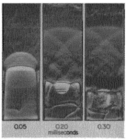
Markstein in 1957 carried out studies of flames traveling inside tubes [39]. During the flame propagation inside a duct, pressure waves are generated (random waves or oscillations). In his paper, Markstein investigated the flame front interaction with a pressure wave generated from the opposite end of ignition of the tube. He used the Schlieren spark photographs, to capture the flame shapes. Fig. 14 shows the flame shapes at the moment of a pressure wave colliding with a flame front. The flame shapes are quite similar to the images of tulip flame formation [39]. He concluded that higher the pressure ratio of the pressure wave generated higher was the radiation of the flame.

Fig. 14: Initial stages of the shock wave flame and front interaction with three images showing the stages of the

development of the tulip flame: image published in [39]

Ignition End

Fig. 13: High speed images of a propagating wave in a closed duct by Ellis in 1928: image

published in [37]