[NORMAL] Comparative Analysis of Point-based and Kernel-based Object Identification Techniques

ISSN (Print): 2320-9798

I

nternational

J

ournal of

I

nnovative

R

esearch in

C

omputer

and

C

ommunication

E

ngineering

(An ISO 3297: 2007 Certified Organization)

Vol. 4, Issue 8, August 2016

Comparative Analysis of Point-based and

Kernel-based Object Identification

Techniques

Mayur Rahul

Assistant Professor, Dept. of CA, UIET, CSJMU, Kanpur (UP), India

ABSTRACT:Object Detection and Recognition are most important problems in Image Processing and Computer

Vision. A lot of research has been done in this field but still intelligent, efficient, robust, usable, and dynamic object detection and recognition methods are unavailable. The accuracy level of the algorithms are very low. This paper compares the various techniques of object identification and recognition, and also describes the comparative analysis of point and kernel based object identification techniques. Most important works are discussed and highlighted. Each methods are discussed according to their pros and cons. The objective of this paper is to present the paper as a useful quick overview and helpful as a beginner’s guide for object identification field. Based on the content presented here, researchers can choose a technique suitable for their own specific object identification problem and further optimizes the chosen technique for better accuracy in object identification.

KEYWORDS: Kalman filter, Particle filter, Discrete-data linear filtering problem, SVM, Multiple hypothesis tracking

I. INTRODUCTION

Object identification is a very challenging and useful problem in the field of computer vision. Object identification is the method of identifying various objects in an image. Good results have been achieved in images but problems remains unsolved in moving images or videos, in particular, when many objects are moving in different places. As an example, it might be easy to train a ball to recognise the presence of wall with nothing else in the image. On the other hand difficulty of finding the path of the ball when there are so many things like table, chair, table-lamp etc. The calculation of path or trajectory is very difficult in such scenario. No effective solutions have been generated so far for this problem.

A lot of research has been done in object identification and recognition during the last few years. The research on object identification is the combination of various disciplines like image processing, machine learning, linear algebra ,topology etc. The research found in this field is so complex that getting beginner’s summary of most of the state-of-the-art approaches are very difficult and time consuming. The objective of this paper is to give the brief summary to the beginners of this field.

This paper briefly summarizes the various aspects of object identification and the main steps involved for most object identification systems. Next section provides the description of various techniques used in object identification .Section 3 describes comparative analysis and last section describes the conclusion.

II. DESCRIPTION

Video is the sequence of images and each image is called frames.Object identification is the process to identify a moving object in a given sequence of frames.The identification of moving object or finding region of interest in the video is the first step in many computer vision applications like medical imaging, video compression,traffic control systems and in wildlife, A video sequence can be divided into two object i.e. foreground object and background object.The moving object like cars,pedestrians are foreground objects and anything behind this is called background object. According to various literatures, the most common steps for object identification are Object detection,Object classification and Object identification itself. Object identification has done according to following reasons:

ISSN (Print): 2320-9798

I

nternational

J

ournal of

I

nnovative

R

esearch in

C

omputer

and

C

ommunication

E

ngineering

(An ISO 3297: 2007 Certified Organization)

Vol. 4, Issue 8, August 2016

(3) According to motion, appearance and shape

So many techniques are available according to above features. Some of which are (1) Point-based

(2) Kernel-based (3) Silhouette-based

In this paper, we are going to compare two methods i.e. point-based and kernel-based. Description of both of these two techniques are explained below.

Point-based Identification:In point-based identification approach, objects are represented as point and generally

scattered at their frames by evolving their motion and position. Point-based identification can be done with the help of Kalman filter, Particle filter and Multiple hypothesis method.

Kalman Filter Method:Kalman filter technique is used to guess the state of a linear system where state is assumed to

be distributed by a Gaussian [1].In 1960, R.E. Kalman published a well-known paper describing a recursive solution to the discrete-data linear filtering problem[2]. Object identification is the process of estimating the object’s position from the previous information and verifying the existence of the object at the estimated position. Further the observed function and motion model must be learnt by some sample of image sequences before identification is performed [3].

The Kalman filter is a set of mathematical equations that provides an efficient recursive environment to predict the state of a process .It is also used to predict past, present and future states. It also predict the states even if there is a lack of description of the nature of the system[4].

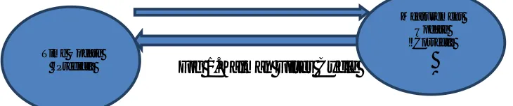
Fig 1.Kalman Filter Cycle

The kalman filter predicts a motion and position by using a form of feedback control. The kalman filter predicts the state at any arbitrary time and then obtains feedback in the form of some noisy measurements. The equations of kalman filter can be categorize into two form :the time update equations and the measurements update equations.The time update equations are responsible for projecting forward(in time) the current state and error covariance estimates to obtain the priori estimate for the next time step.The measurements update equations are responsible for the feedback – i.e. for adding a new measurement into the priori estimate to obtain an improved value of posteriori estimates[8][9].

The time update “prediction” equation[3][4].

State Prediction Xpredk = A* X k-1 + B* U k + W k-1 (1)

Error Covariance Prediction Ppredk = A* P k-1*AT +Q (2) Where

In equation (1)

Xpredk is vector representing predicted process state at time k. A is a 4x4 process transition matrix

A = 1 0 1 0 0 1 0 1 0 0 1 0 0 0 0 1

X is a 4-dimensional vector [ x ydx dy ]

x,y denotes the coordinates of the object’s centre and dx,dy are the velocity. Xk-1 is vector representing process state at time k-1.

Uk is a control vector

Time Update “Predict”

ISSN (Print): 2320-9798

I

nternational

J

ournal of

I

nnovative

R

esearch in

C

omputer

and

C

ommunication

E

ngineering

(An ISO 3297: 2007 Certified Organization)

Vol. 4, Issue 8, August 2016

B relates optional control vector U k into state space.

Wk-1 is a process noise.

In equation (2)

Ppredk is predicted error covariance at time k.

Pk-1 is a matrix representing error covariance in the stateprediction at time k-1

Q is the process noise covariance[

The measurement update “correction” equation:

Kalman Gain K k= P predk * H T *(H * P predk * HT + R) -1 (3) State Update X k = X predk + K k * (Z k - H * X predk ) (4) Error Covariance Update P k = (I – K k * H) * Ppredk (5) In equation (3)

Kk is Kalman gain.

H is matrix converting state space into measurement space R ismeasurement noise covariance.

In equation (4)

Xkis a process actual state.

Using Kalman gain Kk and measurement Zk process state Xkcan be updated.

Zkis the most likely x and y coordinates of the target objects in the frame.

The final step in Kalman filter is toupdate the error covariance Ppredkinto Pk as given in eq. (5). After each time and

measurement update pair, theprocess is repeated with previous posteriori estimates used to project or predict the new priori estimate[5].

Particle Filter Method:The Kalman filter is applicable for state variables which are normally Gaussian distributed. So,

Kalman filter will give poor distributions for the state variables which do not follow Gaussian distribution. Difficulties with kalman filtering will remove by particle filter because it will work easily on non-linear and non-gaussian situations.

Particle filtering is a general Monte Carlo method for performing guess instate-space models where the state of a system evolves in time and information about the state is obtained through noisy measurements made at each time step[10]. In a general discrete-time state-space model, the stateof a system evolves according to:

xk = fk(xk−1, vk−1) (6)

wherexk is a vector representing the state of the system at time k, vk−1 is the state noise vector, fk is apossibly non-linear

and time-dependent function describing the evolution of the state vector. The statevector xk is assumed to be latent or

unobservable. Information about xk is obtained only through noisymeasurements of it, zk, which are governed by the

equation:

zk = hk(xk, nk) (7)

wherehk is a possibly non-linear and time-dependent function describing the measurement process and nk is the

measurement noise vector.The filtering problem involves the estimation of the state vector at time k, given all the measurements up to and including time k, which we denote by z1:k. In a Bayesian process, this problem can be

formalized as the computation of the distribution p(xk|z1:k), which can be done recursively in twosteps. In the prediction

step, p(xk|z1:k−1) is computed from the filtering distribution p(xk−1|z1:k−1) attime k − 1:

p(xk|z1:k−1) = Z p(xk|xk−1)p(xk−1|z1:k−1)dxk−1 (8)

where p(xk−1|z1:k−1) is assumed to be known due to recursion and p(xk|xk−1) is given by Equation 6. The distribution p(xk|z1:k−1) can be thought of as a prior over xk before receiving the most recent measurementzk. In the update step, this

prior is updated with the new measurement zk using the Bayes’ rule to obtainthe posterior over xk:

p(xk|z1:k) / p(zk|xk)p(xk|z1:k−1) (9)

In general, the computations in the prediction and update steps (Equations 8-9) cannot be carried outanalytically, therefore there is the need for approximate methods such as Monte Carlo sampling.

Multiple Hypothesis Method:The measurement to track association is a basic step of a tracking algorithm. This is a

ISSN (Print): 2320-9798

I

nternational

J

ournal of

I

nnovative

R

esearch in

C

omputer

and

C

ommunication

E

ngineering

(An ISO 3297: 2007 Certified Organization)

Vol. 4, Issue 8, August 2016

initialization of a wrong track or deletion of a real track if it has mistakenly notbeen associated with a measurement for one or more scans.When a new set of measurements is calculated by the sensor, each measurement can beassigned to existing track or initiate a new track or to be considered as the wrong alarm. Thesimplest and most widely used technique for measurement to track and its association, is the global nearest neighbour algorithm (GNN) [11]. This technique formulates the most nearest track to measurement and new track hypotheses. In theJoint Probabilistic Data Association (JPDA) algorithm[12],measurement hypotheses are generated for multiple track. Hypotheses probabilities are calculated and theneach track for assignment hypotheses are merged. Track state is updatedusing all the measurements that are within the track gate by using a weighted sum of eachhypothesis track estimate using this method. These two methods are used to form one track estimate for each trackhypothesis. So, GNN and JPDA methods are very efficient in order to take a decision on the current scan incases of conflicting measurement to track association hypotheses.

On the other hand, Multiple Hypotheses Tracking (MHT) methods form alternative association hypotheses in case of observation to track conflict situations. The set ofhypotheses is propagated in the next scans with the anticipation that future observationswill resolve assignment ambiguities. This method is divided into two approaches, thehypothesis oriented MHT (HOMHT) and the track oriented MHT (TOMHT).

Kernel Based Identification:In this type of tracking the kernel refers to the object representations of rectangular or ellipsoidal shape and object appearance[13]. The objects are tracked by calculating the motion of the kernel on each frame. These algorithms differ in terms of the appearance representation used, the number of object tracking, and the technique used for estimation of object motion. In real-time, illustration of object using geometric shape is common. But one of the restrictions is that parts of the objects may be left outside of the defined shape while portions of the background may exist inside. This can be detected in rigid and non-rigid objects.This type of identification can be done in simple template matching ,mean shift method and support vector machine.

Simple Template Matching:Simple template matching is a technique in digital image processing for detecting small

parts of an image which match the image template. It can be used in manufacturing as a part of quality control,a way to navigate a mobile robot, or used to detect edges in images.Advanced template matching algorithms allows us to find occurrences of the template regardless of their orientation and local brightness. Template Matching techniques are flexible and relatively straightforward to use, which makes them one of the most popular methods of object localization. Their applicability is limited mostly by the available computational power, as identification of big and complex templates can be time-consuming. Template Matching techniques are expected to address the following need: provided a reference image of an object (the template image) and an image to be inspected (the input image) we want to identify all input image locations at which the object from the template image is present.It is the brute force method for examining the region of interest in video.

A basic method of simple template matching uses a convolution template, stiff to a specific feature of the search image , which we want to track or identify. This technique is useful on grey images. The convolution measure will be highest at places where the template structure matches with the image structure. This method is normally applied by picking first the part of the search image to use as a template. We use the search image S(x,y) where x,y represents the coordinates of each pixel in search image. Further we use the template T(xt , yt) where (xt , yt) represents the

coordinates of each pixel in the template. Further we move the origin of the template T(xt,yt) over each (x,y) point in

the search image , then calculate the sum of products between the coefficients in S(x,y) and T(xt,yt) over the entire area

covered by the template. Considering all positions of the template to the search image . The position with the highest score is the best position. This method is also called linear spatial filtering and the template is called a filter mask. To handle image translation problems using template matching is to compare the intensities of the pixels , using the sum of absolute difference measure. A pixel in the images with coordinates (xs,ys) has intensity Is(xs,ys) and a pixel in the

template with coordinates (xt,yt) has intensity It(xt,yt). Further the absolute difference in the pixel intensities is defined

as the

Diff(xs,ys,xt,yt) = | Is(xs,ys) – It(xt,yt) | (10)

A(x,y) = ∑ ∑ ( + , + , , ) (11)

ISSN (Print): 2320-9798

I

nternational

J

ournal of

I

nnovative

R

esearch in

C

omputer

and

C

ommunication

E

ngineering

(An ISO 3297: 2007 Certified Organization)

Vol. 4, Issue 8, August 2016

Am = ∑ ∑ ( , ) (12)

Mean Shift Method: The mean-shift method is an efficient approach to identify objects whose appearance is defined

by histograms. It is used to identify non-rigid objects like walking man etc.The mean shift procedure was originally presented in 1975 by Fukunaga and Hostetler[15].Effective visual tracking in a video sequence has always been a typical problem in the field of computer vision. Real-time and robustness are the two issues which always effects the performance of the tracking algorithm. In a tracking video sequence, anunknown target should be defined as anything which is interesting to analysis. To select these right features, which play an important role in the tracking object in a video sequences is a very critical task[16-17]. Feature selection is very similar to the object and target representation. We always analyse the object motion to focuses on simple characteristics such as color, texture, shape, geometry and so on. Generally, most of tracking algorithms always use a combination of these features to track an object. In general, these features are selected manually by the user, which depend on the many fields and application area. Yet, the problem of automatic feature selection has brought more and more attention in computer vision and pattern recognition, namely the detection of objects and then to track object in video sequences. As we all known, the object tracking is usual the first step in activities analysis system, including interactions and relationships between objects of interest. Mean shift method is the object tracking algorithm based on color histograms.

Mean shift is a procedure for locating the maxima of a density function given discrete data sampled from that function. It is useful for detecting the modesof this density.This is an iterative method, and we start with an initial estimate x. Let a kernel functionKF(xi-x) be given.This function determines the weight of nearby points for

re-estimation of the mean.a Gaussian kernelon the distance to the current estimate is used,

KF(xi-x) = ( | |∗| | ) (13)

The weighted mean of the density in the window determined by KF

M(x) = ∑_∑∈ ( ) (₍ )₎

∈ ( ) (14)

Where N(x) is the neighborbood of x ,a set of points for which KF(x) ≠ 0

The difference M(x)-x is called mean shift in Fukunaga and Hostetler[15].The mean-shiftalgorithm now sets x=M(x), and repeats the estimation until M(x) converges.

Support Vector Machine:In machine learning, support vector machines are supervised learning models with

associated learning algorithms that analyze data used for classification and regression analysis[14]. Given a set of training examples, each marked for belonging to one of two categories, an SVM training algorithm builds a model that assigns new examples into one category or the other, making it a non-probabilistic binary linear classifier. An SVM model is a representation of the examples as points in space, mapped so that the examples of the separate categories are divided by a clear gap that is as wide as possible. New examples are then mapped into that same space and predicted to belong to a category based on whichside of the gap they fall on.

Support Vector Machines are based on the concept of decision planes that indicates decision boundaries. A decision plane is one that separates between a set of objects having different class properties. A schematic example is shown in the figure 1. In this example, the objects belong either to GREEN or RED class. The separating line defines a boundary on the right side of which all objects are GREEN and to the left of which all objects are RED. Any new object (white circle) falling to the right is classified as GREEN (or classified as RED if it fall to the left of the separating line).

ISSN (Print): 2320-9798

I

nternational

J

ournal of

I

nnovative

R

esearch in

C

omputer

and

C

ommunication

E

ngineering

(An ISO 3297: 2007 Certified Organization)

Vol. 4, Issue 8, August 2016

The figure 1 is a classic example of a linear classifier. A linear classifier is a classifier that separates a set of objects into their respective groups (GREEN and RED in this case) with a line. Most classification tasks, however, are not that simple, and often more complex structures are needed in order to make an optimal separation, i.e., correctly classify new objects (test cases) on the basis of the examples that are available (train cases). This situation is depicted in the figure 2. Compared to the previous example, it is clear that a full separation of the GREEN and RED objects would require a non-linear curve. Classification tasks based on drawing separating lines to distinguish between objects of different class memberships are known as hyperplane classifiers. Support Vector Machines are used to handle such tasks.

Figure 2

III.COMPARATIVE ANALYSIS

After surveying lots of paper, different methods are explained which are used in point-based and kernel-based object identification techniques. Their comparisons are given in the table no. 1 given below:

Techniques Methods Used Comparison

Point-based Kalman Filter 1.The algorithm is recursive.

2.It can estimate the entire internal state. 3.Hidden states and observations are Gaussian. 4.All relations are linear.

Particle Filter 1.The algorithm is non-recursive.

2.Reduces complexity of calculations and having relatively high accuracy. 3.Hidden states and observations are non-gaussian.

4.All relations are non-linear. Multiple Hypothesis 1.The algorithm is non-recursive.

2.Used to track conflict situations.

3.Track oriented MHT maintains a set of tracks which are not compatible. 4.Hypothesis oriented MHT maintains a set of tracks which are compatible.

Kernel-based Simple Template

Matching

1.It is used to detect the small parts of the image. 2.It consumes large amount of computational time. 3.Doesn’t achieve robust performance in complex scenes. 4.Accuracy is high.

Mean Shift Method 1.Acheived very good results to the variation of translation , rotation and scale.

2.It is invented for data clustering.

3.It is based on the target model which is achieved from the color histogram of moving object.

4.It converges very slowly.

Support Vector Machine 1.Achievedsignificantly higher search accuracy than traditional query refinement schemes.

2.Best for classification of images,Hand-written characters, text.

3.It is measured on the basis of their accuracy ratio and percentage of correctly classified observations.

ISSN (Print): 2320-9798

I

nternational

J

ournal of

I

nnovative

R

esearch in

C

omputer

and

C

ommunication

E

ngineering

(An ISO 3297: 2007 Certified Organization)

Vol. 4, Issue 8, August 2016

IV.CONCLUSION

This paper addresses all the major aspects of an object identification framework. We have discussed point-based and kernel-based object identification techniques which are used in video.. For each technique, the technologies in use and the state-of-the-art research works are discussed. The merits and demerits of the works are discussed and key indicators helpful in choosing a suitable technique are also presented. Thus, the paper presents a concise summary of the state-of-the-art techniques in object detection for new researchers or for the beginners of this field. This study provides a preliminary, concise, but complete background of the object detection problem. Thus, based on this study, for a given problem environment and data availability, a proper technique can be chosen easily and quickly. The focus on research can be dedicated to improving or optimizing the chosen technique for better accuracy in the given problem environment. We have also given a comparative analysis for the beginners to choose best technique among them. We think this paper will help many researchers and readers

REFERENCES

[1] Yilmaz ,Alper, Omer Javed and Mubarak Shah. " Object tracking : A survey." Acm Computing Surveys(CSUR) 38.4 (2006):13.

[2] Kalman, R. E.: A new approach to linear filtering and prediction problems, Transaction of the ASMEJournalof Basic Engineering, 35–45, March 1960.

[3] WatadaJunzoMusaZalili , Jain Lakhmi C., and Fulcher John., .," Human Tracking: A State-of-ArtSurvey.", KES 2010, Part II, LNAI 6277, pp. 454–463, 2010.

[4] Welch, G. and Bishop, G.: An introduction to the Kalmann Filter, In University of North Carolina atChapel Hill, Department of Computer Science. Tech. Rep. 95-041, available at

http://russelldavidson.arts.mcgill.ca/e761/kalman-intro.pdf,2004.

[5] Xu, Sheldon, and Anthony Chang. "Robust Object Tracking Using Kalman Filters with DynamicCovariance."http://www.cs.cornell.edu/Courses/cs4758/2011sp/final_projects/spring_2011/Xu_Chang.pdf

[6] http://groups.inf.ed.ac.uk/vision/caviar/caviardata1/

[7] http://www.hitech-projects.com/euprojects/cantata/ datasets_ can tata / dataset.htm.

[8] Greg Welch and Gary Bishop “An Introduction to the Kalman Filter” TR 95-041, Department of Computer Science University of North Carolina at Chapel Hill Chapel Hill, NC 27599-3175 Updated: Monday, July 24, 2006

[9] Greg Welch and Gary Bishop “An Introduction to the Kalman Filter” University of North Carolina at Chapel Hill, Department of Computer Science Chapel Hill, NC 27599-3175, SIGGRAPH 2001 Course 8

[10]EminOrhan,”Particle Filtering”,eorhan@bcs.rochester.edu,August 11, 2012

[11] Blackman, S. Popoli, R.(1999), Design and analysis of modern tracking systems, ArthechHouse,1580530060, Nonvood, MA.

[12]Fortmann, T. Bar-Shalom. Y. Scheffe. M., Sonar tracking of multiple targets usingJointprobabilistic data association, IEEE Journal of Oceanic Engineering, Vol. 8, Iss.3,pp.173 - 184, July 1983

[13]Mr. JoshanAthanesious J; Mr. Suresh P, ”Implementation and Comparison of Kernel and Silhouette Based Object Tracking”, International Journal of Advanced Research in Computer Engineering & Technology, March 2013, pp 1298-1303.

[14]M.Rahul,”A Robust Approach for Detection of Brain Anomalies using MRI”,IJCSIT, Volume 7,Issue 3,pp. 535-538,april 2016,ISSN:2277-128X [15]Fukunaga, Keinosuke; Larry D. Hostetler (January 1975). "The Estimation of the Gradient of a Density Function, with Applications in Pattern Recognition", IEEE Transactions on Information Theory (IEEE) 21 (1): 32–40,2008-02-29.

[16] Collins,R. T, Yanxi Liu and Leordeanu, M, “Online selection of discriminative tracking features”, IEEE Transactions on Pattern Analysis and Machine Intelligence , 2010, Vol. 10, pp. 1631-1643.

[17] Ying-JiaYeh, Chiou-Ting Hsu, “Online Selection of Tracking Features Using AdaBoost”, IEEE Transactions on Circuits and Systems for Video Technology, 2009, Vol. 3, pp. 442-446.

BIOGRAPHY

Mayur Rahulis a Research Scholar in AKTU, Lucknow(UP).He received Master of Computer Application (MCA)