University of Windsor University of Windsor
Scholarship at UWindsor
Scholarship at UWindsor
Electronic Theses and Dissertations Theses, Dissertations, and Major Papers
2012
IMPROVED ESTIMATION STRATEGIES IN MULTIVARIATE
IMPROVED ESTIMATION STRATEGIES IN MULTIVARIATE
MULTIPLE REGRESSION MODELS
MULTIPLE REGRESSION MODELS
Shabnam Chitsaz
University of Windsor
Follow this and additional works at: https://scholar.uwindsor.ca/etd
Recommended Citation Recommended Citation
Chitsaz, Shabnam, "IMPROVED ESTIMATION STRATEGIES IN MULTIVARIATE MULTIPLE REGRESSION MODELS" (2012). Electronic Theses and Dissertations. 419.
https://scholar.uwindsor.ca/etd/419
This online database contains the full-text of PhD dissertations and Masters’ theses of University of Windsor students from 1954 forward. These documents are made available for personal study and research purposes only, in accordance with the Canadian Copyright Act and the Creative Commons license—CC BY-NC-ND (Attribution, Non-Commercial, No Derivative Works). Under this license, works must always be attributed to the copyright holder (original author), cannot be used for any commercial purposes, and may not be altered. Any other use would require the permission of the copyright holder. Students may inquire about withdrawing their dissertation and/or thesis from this database. For additional inquiries, please contact the repository administrator via email
IMPROVED ESTIMATION
STRATEGIES IN MULTIVARIATE
MULTIPLE REGRESSION MODELS
by
Shabnam Chitsaz
A Dissertation
Submitted to the Faculty of Graduate Studies
through the Department of Mathematics and Statistics
in Partial Fulfillment of the Requirements for
the Degree of Doctor of Philosophy at the
University of Windsor
Windsor, Ontario, Canada
c
Improved Estimation Strategies in
Multivariate Multiple Regression Models
by
Shabnam Chitsaz
APPROVED BY
Y. P. Chaubey, External Examiner Concordia University
J. Pathak
Odette School of Business
A.A. Hussein
Department of Mathematics and Statistics
M. Hlynka
Department of Mathematics and Statistics
S. E. Ahmed, Advisor
Department of Mathematics and Statistics
L. Rueda, Chair of Defense School of Computer Science
Declaration of Co-Authorship
I. Co-Authorship Declaration
I hereby declare that this thesis incorporates the outcome of joint research under-taken in collaboration with my supervisor, Professor S. Ejaz Ahmed. In all cases, the key ideas, primary contributions, experimental designs, data analysis and interpreta-tion, were performed by the author, and the contribution of co-author was primarily through the provision of some theoretical results.
I am aware of the University of Windsor Senate Policy on Authorship and I certify that I have properly acknowledged the contribution of other researchers to my thesis, and have obtained written permission from each of the co-authors to include in my thesis.
I certify that, with the above qualification, this thesis, and the research to which it refers, is the product of my own work.
II. Declaration of Previous Publication
This thesis includes two papers that have been published, and another accepted. It will be published on May 31, 2013.
Thesis Publication title/ full citation Publication
Chapter Status
Chapter 2 Ahmed, S. E., Chitsaz, S., Data-Based Adaptive Estimation in an Investment Model. Communications in Statistics-Theory and Methods , 40(19-20), 2011
Published
Chapter 3 Chitsaz, S., Ahmed, S. E., Shrinkage esti-mation for the regression parameter matrix in multivariate regression model. Journal of Statistical Computation & Simulation., 82(2), 2012
Published
Chapter 3 Chitsaz, S., Ahmed, S. E., An improved es-timation in regression parameter matrix in multivariate regression model. Communi-cations in Statistics - Theory and Methods.
Submitted
I certify that I have obtained a written permission from the copyright owner to include the above published materials in my thesis. I certify that the above material describes work completed during my registration as graduate student at the University of Windsor.
I declare that, to the best of my knowledge, my thesis does not infringe upon anyone’s copyright nor violate any proprietary rights and that any ideas, techniques, quotations, or any other material from the work of other people included in my thesis, published or otherwise, are fully acknowledged in accordance with standard referencing practices. Furthermore, to the extent that I have included copyrighted material that surpasses the bounds of fair dealing within the meaning of the Canada Copyright Act, I certify that I have obtained written permission from the copyright owner to include such material in my thesis.
I declare that this is a true copy of my thesis, including any final revisions, as approved by my thesis committee and the Graduate Studies office, and that this thesis has not been submitted for a higher degree to any other University of Institution.
Abstract
The objective of this dissertation is to study properties of improved estimators of the parameters of interest in two different multivariate regression models, analogous to the fixed-X and random-X scenarios of multiple regression and compare the perfor-mance of these estimators with the usual least square estimator. In general, we study restricted versions of the multivariate regression problem based upon constraining the relationship between Y and X in some way where they may be known or unknown to the researcher prior to statistical analysis.
Chapter two contains a study of the properties of improved estimation strategies for the parameters of interest in a capital asset pricing model under a general lin-ear constraint. Asymptotic results of the suggested estimators include derivation of asymptotic bias, asymptotic mean square error, and asymptotic distributional risk. The asymptotic results demonstrate the superiority of the suggested estimation tech-nique. A simulation study is conducted to assess the performance of the suggested estimators for large samples. Both simulation study and data example corroborate with the theoretical result.
In Chapter three, we consider a multivariate multiple regression model when X is a fixed matrix. Here, we propose shrinkage and preliminary test estimation strategies for the matrix of regression parameters in the presence of a natural linear constraint. We examine the relative performances of the suggested estimators under the candidate subspace based on a quadratic risk function and the results are shown. A simulation study is conducted to compare the performance of the suggested estimators and two data examples are also presented. Our analytical and numerical results show that the suggested estimators perform better than the unrestricted estimator under the candidate subspace.
In Chapter four, we consider a multivariate reduced rank regression model when X is random and we propose preliminary test and shrinkage estimation strategies. We investigate the asymptotic properties of the shrinkage and pretest estimators under a quadratic loss function and compare the performance of the suggested estimators under the candidate subspace and beyond. The methods are applied on a real data set for illustrative purposes and a simulation study is also presented.
Acknowledgements
I would like to express my deepest gratitude to my supervisor Dr. Ahmed, who guided me through the development of this research work. This dissertation would not have been completed without his continued academic advice.
I would like to thank the members of my Thesis Committee, Dr. Hlynka and Dr. Hussein for offering constructive suggestions, and to Dr. Pathak from Odette School of Business. Also I am grateful to Dr. Chaubey from University of Concordia for his valuable comments and advice.
I would also like to thank my wonderful fiance and my best friend Mohammadjavd. His support, encouragement, and understanding have turned the last year of my study into a pleasure. We proved that distance cannot, and will not hurt a bond between two people that is based on mutual respect, trust, commitment, and love.
Finally, my deepest gratitude goes to my mother Batoul Pirdel and my father Mahmood Chitsaz, for their love, encouragement, and continuous support. They helped me to believe in myself. Mom and dad, I love you, I am extremely grateful to what you have done for me and I am here because of you!
Contents
Declaration of Co-Authorship iii
Abstract v
Acknowledgements vi
List of Figures xi
List of Tables xii
Abbreviations xiii
List of Symbols xiv
1 Introduction and Literature Review 1
1.1 Introduction . . . 1
1.2 Highlights of Contributions . . . 6
2 Data Based Adaptive Estimation in an Investment Model 10
2.1 Introduction . . . 10
2.2 Candidate Subspace . . . 12
2.3 Proposed Estimation Strategies . . . 14
2.4 Main Results . . . 15
2.4.1 Asymptotic Bias and Risk Analysis . . . 17
2.4.2 Comparison of ˆβJ S+ and ˆβ . . . . 20
2.4.3 Comparison of ˆβJ S+ and ˆβJ S . . . 21
2.4.4 Comparison of ˜β and ˆβJ S . . . . 22
2.4.5 Comparison of ˆβP T and ˆβ . . . 22
2.5 Numerical Study . . . 23
2.5.1 Simulation Study . . . 23
2.5.2 Real Data Example . . . 26
2.6 Concluding Remarks . . . 28
2.7 Appendix: Proof of Main Results . . . 29
2.7.1 Proof of Theorem 2.4.2 . . . 29
2.7.2 Proof of Theorem 2.4.3 . . . 31
2.7.3 Proof of Theorem 2.4.4 . . . 31
2.7.4 Proof of Theorem 2.4.5 . . . 34
3 Estimation Strategies for a Parameter Matrix in a Multivariate Re-gression Model 37 3.1 Introduction . . . 37
3.2 Main Results . . . 45
3.2.1 Two Useful Lemmas . . . 46
3.3 Bias and Risk Analysis . . . 47
3.3.1 Relative Performance of the Estimators . . . 49
3.3.2 Comparison of ˆCSP T and ˆC . . . 51
3.3.3 Comparison of ˆCSP T and ˆCP T . . . . 52
3.3.4 Comparison of ˆCSP T and ˆCS . . . . 52
3.3.5 Comparison of ˜C and ˆCS . . . 53
3.3.6 Comparison of ˆCJ S and ˆC . . . . 53
3.3.7 Comparison of ˆCJ S+ and ˆCJ S . . . . 54
3.3.8 Comparison of ˜C and ˆCJ S . . . 55
3.4 Numerical Study . . . 55
3.4.1 Simulation Study . . . 55
3.4.2 Real Data Example I . . . 57
3.4.3 Real Data Example II . . . 61
3.5 Concluding Remarks . . . 63
3.6 Appendix: Proof of Main Results . . . 64
3.6.1 Proof of Theorem 3.2.1 . . . 64
3.6.2 Proof of Lemma 3.2.1 . . . 65
3.6.3 Proof of Lemma 3.2.2 . . . 66
3.6.4 Proof for Theorem 3.3.1 . . . 67
3.6.5 Proof of Lemma 3.3.1: . . . 69
3.6.6 Proof of Theorem 3.3.2 . . . 71
4 Estimation Strategies for a Parameter Matrix in a Multivariate Re-duced Rank Regression Model 80 4.1 Introduction . . . 80
4.2 Main Results . . . 87
4.3 Asymptotic Bias and Risk Analysis . . . 89
4.3.1 Relative Performance of the Estimators . . . 90
4.3.2 Comparison of ˆBP T and ˆB . . . 93
4.3.3 Comparison of ˆBP T and ˜B . . . . 94
4.3.4 Comparison of ˆBJ S and ˆB . . . . 94
4.3.5 Comparison of ˆBJ S and ˜B . . . 95
4.3.6 Comparison of ˆBJ S+ and ˆBJ S . . . . 96
4.4 Numerical Study . . . 97
4.4.1 Simulation study . . . 97
4.4.2 Real Data Example . . . 100
4.5 Concluding Remarks . . . 102
4.6 Appendix: Proof of Main Results . . . 103
4.6.1 Proof of Theorem 4.2.1 . . . 103
4.6.2 Proof of Theorem 4.3.1 . . . 105
4.6.3 Proof of Lemma 4.3.1 . . . 106
4.6.4 Proof of Theorem 4.3.2 . . . 107
4.6.5 Proof of Theorem 4.3.3 . . . 110
5 Concluding Remarks and Future Research 114 5.1 Future Research . . . 117
Vita Auctoris 124
List of Figures
2.1 R.E of the estimators forn = 30. . . 25
2.2 R.E of the estimators forn = 100. . . 25
3.1 R.E of the estimators forn = 20. . . 58
3.2 R.E of the estimators forn = 40. . . 58
4.1 R.E of the estimators forn = 40. . . 99
4.2 R.E of the estimators forn = 100. . . 99
List of Tables
2.1 R.E of estimators,n = 30. . . 24
2.2 R.E of estimators,n = 100. . . 24
2.3 Estimators of β for nine diversified funds . . . 27
2.4 The relative efficiency of estimators . . . 28
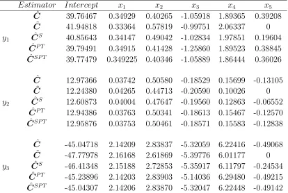
3.1 Estimate of the regression coefficient matrix . . . 60
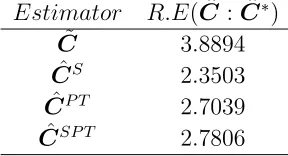
3.2 The relative efficiency of estimators . . . 61
3.3 Estimates of the regression coefficient matrix . . . 62
3.4 The relative efficiency of estimators . . . 63
3.5 Biomedical data on urine samples of patients from a study by Smith et al. (1962). . . 79
4.1 R.E of estimators,n = 40. . . 98
4.2 R.E of estimators,n = 100. . . 98
Abbreviations
ADB Asymptotic distributional bias ADR Asymptotic distributional risk AIC Akaike information criterion
AQDB Asymptotic quadratic distributional bias AN OV A Analysis of variance
AM SE Asymptotic mean square error
B Bias
BIC Bayesian information criterion CAP M Capital asset pricing model
GM AN OV AGeneralized multivariate analysis of variance LS Least square
M AN OV A Multivariate analysis of variance M M RM Multivariate multiple regression model M SE Mean square error
P T pretest estimator QB Quadratic bias
R Risk
RE Restricted estimator R.E Relative efficiency
RRRM Reduced rank regression model U E Unrestricted estimator
SCL Security characteristic line tr Trace of matrix
List of Symbols
θ Regression parameter vector, (intercept), asset’s return
β Regression parameter vector, (slope), asset’s return systematic risk
Ri Return for stock i
Rm Return on the market portfolio
Rf return on treasury note
ε Asset’s nonsystematic risk
H q×pmatrix
h q×1 vector
K r×m matrix
L q×n matrix
A m×r matrix
B r×q matrix
F r1×r matrix
G q×m matrix
D r1×m matrix
V Variance covariance matrix
H0 Null hypothesis
I Identity matrix
L Weighted quadratic loss function
Ω Variance covariance matrix of ε
Σ∗ Variance covariance matrix of restricted estimator
Ω∗ Variance covariance matrix of difference of unrestricted and restricted estimator
Σ12 Covariance matrix between UE and RE
Ω12 Covariance matrix between UE and difference of UE and RE
ˆ
β Unrestricted estimator of regression parameter vector in CAPM ˜
β Restricted estimator of regression parameter vector in CAPM ˆ
βP T Preliminary test estimator of regression parameter vector in CAPM
ˆ
βJ S Shrinkage estimator of regression parameter vector in CAPM
ˆ
βJ S+ Positive shrinkage estimator of regression parameter vector in CAPM
ˆ
C Unrestricted estimator of regression parameter matrix in MMRM ˜
C Restricted estimator of regression parameter matrix in MMRM ˆ
CP T Preliminary test estimator of regression parameter matrix in MMRM ˆ
CJ S Shrinkage estimator of regression parameter matrix in MMRM ˆ
CJ S+ Positive shrinkage estimator of regression parameter matrix in MMRM
ˆ
B Unrestricted estimator of regression parameter matrix in RRRM ˜
B Restricted estimator of regression parameter matrix in RRRM ˆ
BP T Preliminary test estimator of regression parameter matrix in RRRM
ˆ
BJ S Shrinkage estimator of regression parameter matrix in RRRM ˆ
BJ S+ Positive shrinkage estimator of regression parameter matrix in RRRM
Chapter 1
Introduction and Literature
Review
1.1
Introduction
Multivariate multiple regression models (MMRMs) are generalizations of the usual
multiple regression models when several response variables have to be predicted based
on a set of predictor variables. MMRMs have recently found a wide range of
appli-cations in a variety of areas such as artificial intelligence, machine learning theory,
education and psychology. (see for example Izenman (2008) and Timm (2002))
Regression analysis includes many techniques for modeling the relationships among
variables and estimating the parameters of the model. When an estimator is obtained
based on sample data only, it is well known that the maximum likelihood estimation
leads to the best estimate among linear unbiased estimates. We call it an unrestricted
maximum likelihood estimator. However, in problems of statistical inference,
1.1 Introduction 2
times we deal with uncertain prior information or some constraints on some of the
parameters in a statistical model, which usually leads us to an improved inference
based on alternative methods. Now the question arises as to how one can insert this
uncertain prior information into the inference procedure. In this regard, Bancroft
(1944) came up with the idea of testing the uncertainty of the prior information in
the estimation procedure. It is reasonable to perform a pretest or pretest on the
validity of the uncertain prior information and then analyze its development based
on the result of the test. The new estimator that uses uncertain prior information to
find improved estimates is called a restricted estimator. For examples on the results
from many researchers, see Ahmed (2001), Ahmed et al. (2007), Ahmed and Chitsaz
(2011), Chitsaz and Ahmed (2012b), Chitsaz and Ahmed (2012a), and others. We
believe that the restricted estimator is more efficient than the unrestricted estimator
after using prior information. Recent studies are mostly based on estimating the
vector parameter.
The MMRM can be written as
Y =CX +E, (1.1)
where,Y is a full rankn×mmatrix of response variables,X is a full rankq×nmatrix
of predictor variables,Cis a full rankm×qregression coefficients matrix, andEis the
n×mmatrix of random errors. Linear restrictions on the regression coefficients are of
such importance in estimation and testing that a special symbolism has been worked
out. For example, in the analysis of variance, the analyst is concerned with whether
treatment effects are equal, and the economist is often concerned about whether one
or more parameters are zero. Similarly, researchers often wonder whether to pool
1.1 Introduction 3
are equal to a constant.
In this dissertation, we suggest some estimators for the parameter matrix in MMRM
and we concentrate on estimating the parameter matrix, C, under a very general set
of linear constraints as prior information,
H0 :KCL=0, (1.2)
where K and L are known full-rank matrices of appropriate dimensions. Basically,
we consider the estimation problem in two competing models, where one model
in-cludes all predictors and the other restricts variable coefficients to a linear constraint
based on prior information. In this dissertation, we develop some improved
estima-tion strategies such as pretest and shrinkage estimaestima-tion methods for the matrix of a
regression parameter in three different multivariate regression models.
Unrestricted and restricted estimator:
With a set of potential restrictions in mind as prior information , the researcher’s
attention is drawn to two estimators. Let ˆC be the ordinary (unrestricted) least
square estimators ofC, and let ˜Cbe the restricted estimator ofCunder a very general
set of linear constraints as prior information named the candidate subspace (1.2). The
estimator ˜C has a smaller variance than the unrestricted estimator; if the restrictions
are true, ˜C is unbiased. Therefore, imposing false restrictions while reducing variance
leads to bias, and the worse the restriction, the worse the bias. In many cases,
researchers may have restrictions in mind such as pooling data, dropping variables,
and so on. They may not be certain whether the restrictions are valid, or they
may wish the data reveal something about the truth or falsity of the restrictions. A
1.1 Introduction 4
Pretest estimator:
Let D be a test statistic for the null hypothesis in (1.2) and drn,α be the critical
value of the distribution of D under the null hypothesis. We define the following
pretest estimator:
ˆ
CP T = ˆC−( ˆC−C˜)I(D < drn,α),
where thedrn,αis the upperα-level critical value of theχ2 distribution withrndegrees
of freedom, and I(A) is an indicator function of a set A. There is always the chance
of accepting a false hypothesis or rejecting a true hypothesis. When the analyst acts
as if the restrictions are true, he runs a risk associated with a type two error; if the
restrictions are false, he runs a risk associated with the other type of error involved
in hypothesis testing. In general, the pretest estimator is biased, since ˜C is biased
if the restrictions are false, because there is a nonzero probability of accepting false
restrictions via the test. However, the performance of this estimator is substantially
better than the unrestricted estimator when uncertain prior information is nearly
correct. Some useful literature about this estimator can be found in Bancroft (1944),
Albertson (1991), and Ahmed (2001).
Estimators that are better in squared error loss than pretest estimators exist.
Hence, James-Stein type estimators are defined and contrasted with pretest
esti-mators.
Shrinkage and positive shrinkage estimator:
1.1 Introduction 5
parameters matrix based on a James-Stein type estimator is defined as
ˆ
CJ S = ˜C+{1−cD−1}( ˆC−C˜), c >2,
where the optimal value ofcis chosen in an interval in such a way that ˆCJ S dominates ˆ
C. Note that the above estimator is derived by simply replacing the binary function of
I(A) by a continuous functioncD−1. Therefore, this estimator may have the opposite
sign of ˆC. To avoid that, we truncate ˆCJ S to obtain the positive shrinkage estimator
which is defined as
ˆ
CJ S+ = ˜C+{1−cD−1}+( ˆC−C˜), c > 2.
If the candidate subspace as prior information is true, there is no issue since the
imposition of a true candidate subspace reduces variances and does not cause bias.
Imposition of a false candidate subspace introduces bias. Thus, the only way of
making a judgment on listed estimators is to derive a risk function that assigns weights
to bias and variance. We have studied the performance of the suggested estimators
in terms of their risks. In an effort to provide the risk analysis, we considered the
quadratic loss function of the form
L(C∗,C) = [vec(C∗−C)]0W[vec(C∗−C)],
where W is the positive semi-definite (p.s.d) matrix with an appropriate dimension.
Then the risk of C∗ or any estimator ofC is
1.2 Highlights of Contributions 6
where M SE(C∗) = E{vec(C∗ − C)[vec(C∗ − C)]0}. For instance, if we get
M SE(C∗) = (A⊗B) with a Aand B nonsingular matrix, we define the quadratic
risk as follows:
R(C∗;W) =tr(W B)tr(A).
1.2
Highlights of Contributions
The goal of this dissertation is to generalize estimation of the matrix parameter in
MMRM. We describe two different multivariate regression scenarios, analogous to the
fixed X and random X scenarios of multiple regression. We extend the concept of
James-Stein type shrinkage estimation methods and pretest estimation in the context
of three different linear regression models.
In Chapter two, we consider the simple multivariate regression model that includes
basic investment models. For that, we have studied the capital asset pricing model
which reflects how the expected return on an asset is a function of the expected
returns on the market, the risk-free asset, and of the relevant risk of that asset. The
goal of this model is to describe the properties of having an optimal portfolio given
the best selection of stock for investors who like more return and less risk. Let us
consider a system of regression models derived from a capital asset pricing model.
yt=θ+xtβ+t, t= 1,· · · , n, (1.4)
whereytis thep×1 vector of excess return onk assets; letxtbe the excess return on
the market portfolio at timet. Here, the parameterβ is the regression slope between
1.2 Highlights of Contributions 7
to the market. Here, the goal is to maximize the performance of a portfolio when
it is prior suspected that the asset’s return, θ, may be restricted to a subspace. In
this scenario, we are dealing with different estimation strategies for the parameters
in a simple multivariate regression model. Here we consider alternative estimators of
the slope parameter in a regression model with a non-normal error when uncertain
prior information about the value of the intercept parameter is available and can be
expressed in the general form of a null hypothesis, Hq×pθp×1 = hq×1. We develop
a large sample theory for the estimators that includes derivation of asymptotic bias
and asymptotic distributional risk of the suggested estimators. The asymptotic results
demonstrate the superiority of the suggested estimation technique. Also, a simulation
study shows that the method suggested here has sound finite sample properties and
strongly corroborates with the theoretical results of this chapter. A data example is
also presented to illustrate the suggested estimation strategies.
In Chapter three, we generalize the estimation strategies for the matrix of a
re-gression parameter in a multivariate multiple rere-gression model in the presence of a
natural linear constraint when the matrix of predictor variables X is fixed and non
stochastic. Also, we study the application of shrinkage and pretest estimation
strate-gies in MMRM, which is the most important model for many practical situations.
The goal is to critically examine the relative performances of the listed estimators in
the direction of the subspace and candidate subspace restricted type estimators. In
the case of multivariate multiple regression, we are dealing with the parameter
ma-trix estimation. So, the fundamental results of Sclove et al. (1972) cannot be directly
implemented to compute the expressions needed to check the validity and relative
efficiency of proposed estimators under very general linear constraints. Therefore, we
1.2 Highlights of Contributions 8
expressions for the suggested estimators. This chapter also addresses the pairwise
comparisons of the proposed estimators. Our analytical and numerical results show
that, overall, the proposed shrinkage estimators perform the best. The methods are
also applied on a real data set for illustrative purposes.
However, there are many problems in multivariate statistical analysis that involve a
test concerning regressions of reduced rank and restrictions on regressions. Therefore,
the special feature that can be entered into the multivariate linear regression model
case is that we admit the possibility that the rank of the regression coefficient matrix
can be deficient. This implies that there are linear restrictions on the coefficient
matrix, and these restrictions themselves are often not known a priori. Such a model is
called a reduced rank regression model. The model structure and estimation strategies
for this model will be explicitly discussed in Chapter four of this dissertation. Note
that in this chapter we consider the predictor variables X to be random.
In model (1.2) when C has reduced rank r, there exist two non-unique full rank
matrices: an (m×r) matrix A and an (r×q) matrix B, such that C = AB. We
restate the model in (1.2) as a reduced rank regression model, such that
Y =ABX +E. (1.5)
The above mentioned features have practical implications. When we model with a
large number of response and predictor variables, the implication in terms of
restric-tions serves a useful purpose. Certain linear combinarestric-tions of response variables can,
eventually, be ignored for regression modeling purposes, since these combinations will
be found to be unrelated to the predictor variables. The alternative implication
1.2 Highlights of Contributions 9
in the regression model, since any remaining linear combinations may be found to have
no influence on the response variables given the first set of linear combinations. Thus,
the reduced rank regression procedure takes care of the dimension reduction aspect
of a multivariate regression model when building through the assumption of a lower
rank for the regression coefficient matrix. Statistical problems concerning reduced
rank regression models have been studied in the statistical literature by Anderson
(1951, 1984), Srivastava and Khatri (1979), (see Chapters 5 and 6), Muirhead and
Koole (1982), (see Chapter 10), Reinsel (1998), Heinen and Rengifo (2007), Vounou
et al. (2010), and others.
Therefore, in many practical situations, there is a need to reduce the number of
parameters in model (1.2), and we approach this problem through the assumption of
a lower rank of the matrix B in model (1.5) caused by linear constraints defined by
FBG =D. (1.6)
In Chapter four, we consider shrinkage and pretest estimators in multivariate
re-duced rank regression model. We investigate the asymptotic properties of suggested
estimators under a very general candidate subspace. In the support of our analytical
results, we present a data example and simulation study.
Chapter five summarizes the results, and concludes the dissertation with a
Chapter 2
Data Based Adaptive Estimation
in an Investment Model
2.1
Introduction
The capital asset pricing model (CAPM), or Sharpe-Lintner model, stands out among
asset pricing models. This model reflects how the expected return on an asset is a
function of the expected returns on the market, the risk-free asset, and the relevant
risk of that asset. The goal of the CAPM is to describe the properties of having an
optimal portfolio given the best selection of stocks for any investors who like more
return and less risk. The Portfolio theory describes the process by which investors
seek the best possible portfolio in terms of the tradeoff of risk for return. Portfolio
management involves deciding what assets to include in the portfolio, how many to
purchase, and when to purchase them. For this purpose, Jensen (1968) studied a
2.1 Introduction 11
regression model of the CAPM, given below:
Rit−Rf =θi+βi(Rmt−Rf) +εit,
where Rit is the return for stock i in period t, Rf is the return of treasury note, θi
is an asset’s return in a access of it’s risk adjusted, βi is an asset’s systematic risk
for stock i, Rm is the return on the market portfolio in periodt, andεit is the asset’s
nonsystematic risk in period t. In this chapter, we consider a system of regression
models derived from a capital asset pricing model.
yt=θ+xtβ+t, t= 1,· · · , n. (2.1)
Let yt be the p× 1 vector of excess return on k assets, and let xt be the excess
return on the market portfolio at time t. For the inference purpose, we assume that
E(t) = 0, Cov(t) = Ω, and E(xtt) = 0. Here, the parameter β is the regression
slope between the asset return and that of the market (security characteristic line,
(SCL)), which shows how a stock acts in relation to the market. The measure of
the sensitivity of the asset return to the market movement is given so that market
variance is equal for all the assets. We will call a security an “aggressive security” if
its beta exceeds 1,“βi >1”, and “defensive” if its beta falls below 1, “βi < 1”. The
factor θ of the ith risk asset represents the difference between the expected return
according to the observed reality and the expected return according to the CAPM
theory. Now, if the estimated θ is significantly positive or negative, then the given
risk asset produces returns that are over or below the appropriate values following
the theory. Thus, in the market, the asset seems to be either underestimated or
2.2 Candidate Subspace 12
a higher average return for a given risk, and a lower risk for a determined average
return. It would be beneficial, if we have some preliminary information about θ,
to have better estimation for the systematic risk and more efficient portfolio with
more returns. The goal of this chapter is to maximize the performance of a portfolio
when it is prior suspected that the asset’s return,θ, may be restricted to a subspace.
Ahmed and Krzanowski (2004) have considered estimation of the intercept vector
in a simple multivariate normal regression model when it is a priori suspected that
the slope vector may be restricted to a subspace. In this chapter, we investigate this
problem when there is no assumption about the error term, and the prior information
about the value of the intercept parameter can be expressed in the general form of a
null hypothesis, Hθ =h.
2.2
Candidate Subspace
Let the candidate subspace be defined by Hq×pθp×1 =hq×1 and Ω=σ2V. WhenV
is known and nonsingular, then the weighted least square estimators (WLSE) of β
and θ are given by
ˆ β =
n
X
t=1
(xt−x¯)yt/ n
X
t=1
(xt−x¯)2
and
ˆ
θ= ¯y−x¯βˆ.
However, even when V is unknown, the estimator of β does not depend on V; V
drops out of since the covariate is scalar. Now, considering the problem of finding ˜
2.2 Candidate Subspace 13
Lagrangian function whereλ is an q×1 vector of Lagrange multipliers:
` =X
t
(yt−θ−xtβ)0V−1(yt−θ−xtβ) + 2λ0(Hθ−h).
Differentiation with respect toθ, β and λ yields the following results:
˜
β= ˆβ+C(Hθˆ−h),
where
C =dV H0(HV H0)−1
and
d= Pn nx¯
t=1(xt−x¯)2
.
Note that HV H0 is invertible. We call ˜β a candidate sub-model or a restricted
esti-mator ofβ. ˜β will be equal to ˆβ, an unbiased estimator, if the subspace information
is correct i.e. Hθ = h. Therefore, ˜β will be a biased estimator if the subspace
information is not correct. On the other hand, it will be relatively more efficient than
the classical estimator ˆβ when such subspace information represents the data.
A useful but compromising method for tackling the uncertainty regarding the
subspace information is to implement estimation strategies based on shrinkage and
pretest principles. For point estimation, we refer to Ahmed (2001), Khan and Ahmed
(2003), and Ahmed et al. (2010), among others. For the purpose of statistical inference
in such cases, one could employ an empirical Bayes approach to the computation of
standard errors of these shrinkage estimators; for example, see Maddala et al. (1997).
Alternatively, Kazimi and Brownstone (1999) proposed confidence bands for
2.3 Proposed Estimation Strategies 14
have proposed the use of mean squared error matrices with a class of shrinkage
esti-mators for the purposes of constructing confidence ellipsoids.
The remainder of this chapter is organized as follows. In Section 3, pretest and
shrink-age estimators are defined. In Section 4, we derive the expressions for asymptotic bias
and risk of the proposed estimators, and provide their relative performances. Section
5 provides a simulation study and a real data example. Conclusions are offered in
Section 6. Finally the proof of the main results are provided in Section 7.
2.3
Proposed Estimation Strategies
Here, we consider pretest and shrinkage estimations of the regression parameter vector
β. The pretest estimator is defined as
ˆ
βP T = ˆβI(P > χ2q,α) + ˜βI(P ≤χ2q,α),
whereI(A) is an indicator function of the set A, andP is the test statistic for testing
Hθ =h as given by
P =s2e( ˆβ−β˜)0M−1( ˆβ−β˜)
where
M = (1 n +
¯ x2
Q)CHV H 0
C0.
When the subspace information is true, (Hθ =h), the statistic P follows χ2
distri-bution with q degrees of freedom asn → ∞.The James-Stein or shrinkage estimator
as a smooth function of P is given by
ˆ
2.4 Main Results 15
Notice that ˆβJ S is similar to ˆβP T where we have replaced the indicator function
I(P ≤ χ2
q,α) by a continuous decreasing function mP
−1 of P. Thus, instead of two
extreme choices, namely ˆβor ˜β, ˆβJ S provides the choice for all values between ˆβ and
˜
β depending on the value of P for a given sample. Here, mis the shrinkage constant
and is chosen in an interval in such a way that ˆβJ S dominates ˆβ in terms of risk. m
is allowed to vary over [0,2(q−2)), q > 2, often set to m = q−2; thus, we assume
that q ≥3. We can see that ˆβJ S tends to ˆβ asP tends to infinity, and it tends to ˜β as P →q−2. Finally, the positive-part shrinkage estimator is
ˆ
βJ S+ = β˜+ (1−mP−1)+( ˆβ−β˜),
where z+=max(0, z), or, equivalently, as
ˆ
βJ S+= ˜β+ (1−mP−1)I(P > m)( ˆβ−β˜).
Having defined all these estimators, we investigate their asymptotic properties in the
following section.
2.4
Main Results
Letν1 =
√
n( ˆβ−β),ν2 =
√
n( ˜β−β), andν3 =
√
n( ˆβ−β˜). To establish the
asymp-totic properties of listed estimators, we consider the local alternatives to guarantee
convergence and overcome the difficulty of identical asymptotic distribution of some
listed estimators in large samples under fixed alternatives. To do so, we consider a
sequence of local alternatives {Ln} defined by Ln : Hθ =h+√ξn, where ξ is a real
2.4 Main Results 16
need the following three regularity conditions for the asymptotic normality of (θ,β)
as n→ ∞.
Theorem 2.4.1. Consider the simple regression model when the components of the
error vector = (1, . . . , n)0 are independent, E(t) = 0, Cov(t) = σ2V, and the
distribution of is non-normal. Now assume the following regularity assumptions:
(i) limn→∞x¯= ¯x0, |x¯0|<∞
(ii) Let qt=xt−√x¯Q then max1≤t≤nqt2 →0 as n → ∞.
(iii) Let Q=
n
X
t=1
(xt−x¯)2. Then limn→∞n−1Q=Q0 <∞.
Then,
√
n( ˆθ−θ)
√
n( ˆβ−β)
∼N2p
( 0 0 , σ 2 V
(1 + Qx¯2
0) − ¯
x Q0
− x¯
Q0 Q −1 0 ) .
Theorem 2.4.2. Under assumed regularity conditions given in Theorem 2.4.1 and
{Ln}, we have
(i) ν1 ν2 ∼N2p
( 0 γ , σ 2
Q−01V Σ12
Σ21 Σ∗
) (ii) ν1 ν3 ∼N2p
( 0 −γ , σ 2
Q−01V Ω12
Ω21 Ω∗
)
whereγ=Cξ,Q=
n
X
t=1
(xt−x¯)2,Σ∗ =Q−01V +(1+ ¯
x2
Q0)CHV H
0C0−2¯xQ−1
0 CHV,
Σ12 = Σ021 = Q
−1
0 V − xQ¯
−1
0 CHV, Ω12 = Ω021 = ¯xQ
−1
0 CHV, and Ω
∗ = (1 +
¯
x2
Q0)CHV H 0C0.
2.4 Main Results 17
2.4.1
Asymptotic Bias and Risk Analysis
In this section, we obtain expressions for the asymptotic distributional bias (ADB)
and the risks (ADR) of the proposed estimators. Also, we compare the performance
of the suggested estimators in terms of asymptotic bias and risk, respectively. Here,
we present the expression for the asymptotic distribution bias (ADB) of the proposed
estimators. The ADB of an estimatorβ∗ is defined as
ADB(β∗) = lim
n→∞E
n
n12(β∗−β)
o
.
To study the asymptotic quadratic risks of the estimators, we define a quadratic
loss function using a positive definite matrix (p.d.m.) W, namely
L(β∗,β) =n(β∗−β)0W(β∗−β),
where β∗ is any one of ˆβ, ˜β, ˆβP T, ˆβJ S, and ˆβJ S+.
Now we assume that for the estimatorβ∗ ofβ the cumulative distribution function
of β∗ under {Ln} exists and can be denoted as F(x) = limn→∞P{
√
n(β∗ −β) ≤
x|Ln}, where F(x) is nondegenerate. Then, the ADR of β∗ is defined as
ADR(β∗,W) = tr
W
Z
Rp1
Z
xx0dF(x)
= tr(W Z),
where Z is the dispersion matrix for the asymptotic distribution F(x). We say
that ˆβ dominates ˆβ? for all β, if ADR( ˆβ;W)< ADR( ˆβ?;W).
pro-2.4 Main Results 18
posed estimators are respectively
ADB( ˜β) = γ
ADB( ˆβP T) = γHq+2(χ2q(α),∆)
ADB( ˆβJ S) = mγE(χ−q+22 (∆))
ADB( ˆβJ S+) = ADB( ˆβJ S)−γE{(mχq−+22 (∆)−1)I(χ2q+2(∆)< m)},
where γ = Cξ, m = q−2, and the notation Hν(x; ∆) is the distribution function
of non-central chi-square distribution with ν degrees of freedom and non-centrality
parameter ∆ =Q0σ−2(γ0V−1γ).
Proof: See Appendix, Section 2.7.2.
Since the asymptotic bias expression of all the estimators are not in scalar form,
we therefore take the recourse of converting them into the quadratic form. Thus, let
us define the asymptotic quadratic distributional bias (AQDB) of an estimator β∗ of
β by
AQDB(β∗) =Q0σ−2[ADB(β∗)]0V−1[ADB(β∗)].
Based on the above, we can easily obtain the AQDB of the estimators.
AQDB( ˜β) = ∆
AQDB( ˆβP T) = ∆{Hq+2(χ2q(α),∆)}
2
AQDB( ˆβJ S) = m2∆{E(χ−q+22 (∆))}2
AQDB( ˆβJ S+) = ∆{mE(χ−q+22 (∆))−E{(mχ−q+22 (∆)−1)I(χ2q+2(∆)< m)}2.
2.4 Main Results 19
size ofα and ∆. The asymptotic bias of ˆβJ S and ˆβJ S+
depend on ∆ alone. Thus, we
can establish the following relation:
0 =AQDB( ˆβ)≤AQDB( ˆβJ S+)≤AQDB( ˆβJ S)≤AQDB( ˆβP T)≤AQDB( ˜β).
Theorem 2.4.4. Under {Ln}, the asymptotic covariance matrices (AMSE) of the
estimators are as follows:
AM SE( ˆβ) = Q−01V
AM SE( ˜β) = Q−01V +G−2F +γγ0
AM SE( ˆβP T) = Q−01V + [G−2F]Hq+2(χ2q(α),∆)
+ γγ0{−2AHq+2(χ2q(α),∆)
− 2AHq+4(χ2q(α),∆) +Hq+4(χ2q(α),∆)}
AM SE( ˆβJ S) = Q0−1V +m2GE(χq−+24 (∆))−2mF[E(χ−q+22 (∆))] +mγγ0
[−2AE(χ−q+42 (∆))−2AE(χ−q+22 (∆)) +mE(χ−q+44 (∆))]
AM SE( ˆβJ S+) = AM SE( ˆβJ S)−G[E(1−mχ−q+22 (∆))2I(χ2q+2(∆) < m)]
+ γγ0{2E(1−mχ−q+22 (∆))I(χ2q+2(∆)< m)−E(1−mχ−q+42 (∆))2
× I(χ2q+4(∆)< m)},
where A=G−1F, G=Ω∗, and F =Ω
12.
Proof: See Appendix, Section 2.7.3.
The asymptotic risk expressions for the estimators are contained in the following
theorem.
fol-2.4 Main Results 20
lows:
ADR( ˆβ;W) = Q−01tr(W V),
ADR( ˜β;W) = Q0−1tr(W V) +a×tr(Z11)−2b×tr(W CHV) +η10Z11η1
ADR( ˆβP T;W) = Q0−1tr(W V) + [a×tr(Z11)−2b×tr(W CHV)]Hq+2(χ2q(α),∆)
− 2tr(W γγ0A)[Hq+2(χ2q(α),∆) +Hq+4(χ2q(α),∆)]
+ η01Z11η1Hq+4(χ2q(α),∆))
ADR( ˆβJ S;W) = Q−01tr(W V)−2mb×tr(W CHV)E(χ−q+22 (∆))
− 2m×tr(W γγ0A)[E(χq−+42 (∆)) +E(χ−q+22 (∆))]
+ am2×tr(Z11)E(χ−q+24 (∆)) +m
2η0
1Z11η1E(χ−q+44 (∆))]
ADR( ˆβJ S+;W) = ADR( ˆβJ S;W)−a×tr(Z11)[E(1−mχ−q+22 (∆)) 2
I(χ2q+2(∆) < m)]
+ η01Z11η1{2E(1−mχ−q+22 (∆))I(χ 2
q+2(∆)< m)−E(1−mχ
−2
q+4(∆)) 2
× I(χ2q+4(∆)< m)},
where a= (1 + Qx¯2
0) andb = ¯xQ −1
0 .
Proof: See Appendix, Section 2.7.4.
2.4.2
Comparison of
β
ˆ
J S+and
β
ˆ
Let us consider the risk of ˆβJ S+ under a subspace, in terms of the risk of ˆβ:
ADR( ˆβJ S+;W) = ADR( ˆβ;W)−2mb×tr(W CHV)E(χ−q+22 (0))
+ a×tr(Z11){m2×E(χ−q+24 (0))−E[(1−mχ
−2
q+2(0)) 2
]
2.4 Main Results 21
Since {E(1−mχ−q+22 (0))2I(χ2
q+2(0)< m)} ≤E[(1−mχ
−2
q+2(0))2] and the expectation
of a positive random variable is positive, then, for allm satisfying the condition
tr(Z11)>
2mb×tr(W CHV)E(χ−q+22 (0)) a[m2×E(χ−4
q+2(0))−E(1−mχ
−2
q+2(0))2]
,
ˆ
β performs better than ˆβJ S+. However, as ∆ increases, ˆβJ S+ dominates ˆβ outside
an interval near the origin.
2.4.3
Comparison of
β
ˆ
J S+and
β
ˆ
J SFor comparing the asymptotic risk of ˆβJ S and ˆβJ S+, we consider the risk difference
of them
ADR( ˆβJ S;W)−ADR( ˆβJ S+;W) = a×tr(Z11)[E(1−mχ−q+22 (∆))
2I(χ2
q+2(∆) < m)]
− η10Z11η12E(1−mχ−q+22 (∆))I(χ
2
q+2(∆)< m)
+ η10Z11η1E(1−mχ−q+42 (∆))
2I(χ2
q+4(∆) < m),
since the expectation of a positive random variable is positive and, by the definition
of an indicator function, the first and last terms are positive. For the second term in
the equation, we observe that (0 < χ2
q+2(∆) < m) ⇐⇒(mχ
−2
q+2(∆)−1) ≥0, we get
E[(1−mχ−q+22 (∆))I(χ2
q+2(∆) < m)] ≤ 0. Thus, the second term is nonnegative too.
2.4 Main Results 22
2.4.4
Comparison of
β
˜
and
β
ˆ
J SWe investigate the risk-difference of ˆβJ S and ˜β under subspace is
ADR( ˜β;W)−ADR( ˆβJ S;W) = 2b×tr(W CHV)(m−1)−am2×tr(Z11)E(χ−q+24 (0))
the risk of ˆβJ S is smaller than ˜β when the condition
tr(W CHV)> am
2 ×tr(Z
11)E(χ−q+24 (0))
2b(m−1) .
Thus, ˆβJ S does not dominate ˜β under a subspace. However, for the large values of ∆, the reverse conclusion holds.
2.4.5
Comparison of
β
ˆ
P Tand
β
ˆ
The risk difference is given by
ADR( ˆβ;W)−ADR( ˆβP T;W) = −[a×tr(Z11)−2b×tr(W CHV)]Hq+2(χ2q(α),∆)
+ 2tr(W γγ0A)[(Hq+2(χ2q(α),∆) +Hq+4(χ2q(α),∆))]
− η10Z11η1Hq+4(χ2q(α),∆))
The right hand side is nonnegative whenever
η10Z11η1 <
[2b×tr(W CHV)−a×tr(Z11)]Hq+2(χ2q(α),∆)
Hq+4(χ2q(α),∆)
,
In this range, ˆβP T performs better than ˆβ as well as under the null hypothesis
2.5 Numerical Study 23
After comparing the ADR of all the estimators, we can see that
ADR( ˆβJ S+;W)≤ADR( ˆβJ S;W)≤ADR( ˆβ;W).
Also comparing the ˆβP T with ˆβ, we see that ADR( ˆβP T;W)≤ADR( ˆβ;W).
2.5
Numerical Study
2.5.1
Simulation Study
In this section, we use Monte Carlo simulation experiments to examine the
perfor-mance of the proposed estimators based on a moderate and a large sample
method-ology. In this study, we simulate data from the following model:
yt1
yt2
= θ1 θ2 +xt
β1 β2 +
εt1
εt2
t= 1,· · · , n.
For simulation, we consider θ = (1.5,2.5), H = ((1,0)0,(0,1)0)0, and h = (1.5,2.5).
Under the candidate subspace, we generate 5000 samples using the above model,
which is adequate since a further increase in the number of replications did not
sig-nificantly change the result. We define ∆ as a departure parameter which is a function
of the distance between the true value of θ and that under the null hypothesis. In
order to investigate the behavior of the proposed estimators, different values of θ
were chosen to produce the value of ∆ between 0 and 4. The performance of an
estimator of θ will be reappraised using the mean square error criterion. All
2.5 Numerical Study 24
the relative risk of ˜β, ˆβP T, ˆβJ S, and ˆβJ S+ with respect to ˆβ by simulation. The
simulated relative efficiency of the estimator β∗ to the unrestricted ˆβ is defined by
R.E =risk( ˆβ)/risk( ˆβ∗).We applied our method to several simulated data sets, and
the results were similar. Since the result for different n were similar, here we only
report the results for n = 30 and n = 100 in Tables 2.1 and 2.2, and Figures (2.1)
and (2.2).
Table 2.1: R.E of estimators, n = 30.
∆ β˜ βˆP T βˆJ S βˆJ S+ 0.0 3.198 2.449 1.323 1.467 0.2 2.199 1.410 1.020 1.320 0.4 1.104 0.85 1.065 1.115 0.6 0.621 0.898 1.051 1.054 0.8 0.381 0.883 1.029 1.029 1.2 0.181 0.894 1.015 1.015 1.6 0.105 1.000 1.009 1.009 2.0 0.067 1.000 1.006 1.006 4.0 0.017 1.000 1.001 1.001
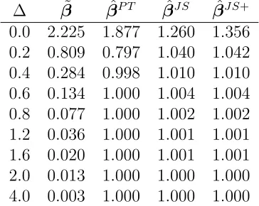
Table 2.2: R.E of estimators, n= 100.
∆ β˜ βˆP T βˆJ S βˆJ S+
0.0 2.225 1.877 1.260 1.356 0.2 0.809 0.797 1.040 1.042 0.4 0.284 0.998 1.010 1.010 0.6 0.134 1.000 1.004 1.004 0.8 0.077 1.000 1.002 1.002 1.2 0.036 1.000 1.001 1.001 1.6 0.020 1.000 1.001 1.001 2.0 0.013 1.000 1.000 1.000 4.0 0.003 1.000 1.000 1.000
2.5 Numerical Study 25
0.0 0.5 1.0 1.5 2.0
0.0
0.5
1.0
1.5
2.0
2.5
3.0
3.5
Δ
RE
Unres RE PT JS JS+
Figure 2.1: R.E of the estimators for n= 30.
0.0 0.5 1.0 1.5 2.0
0.0
0.5
1.0
1.5
2.0
2.5
Δ
RE
Unres RE PT JS JS+
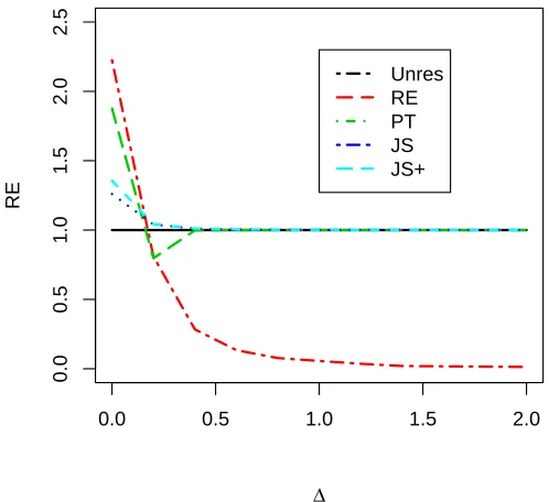
2.5 Numerical Study 26
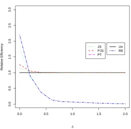
value of the departure parameter ∆. The tables and figures reconfirm the typical
characteristics of the listed estimators. We conclude that ˜β and ˆβP T dominate the
usual ˆβ at and near the candidate subspace. ˆβJ S and ˆβJ S+ are more efficient than
an unrestricted one in the unrestricted parameter space. If the candidate subspace is
correctly specified, that is, ∆ = 0 or in the neighborhood of that, then the ˆβP T is more
efficient than ˆβJ S and ˆβJ S+. However, for a larger value ofα, the level of significance, ˆ
βJ S+ dominates ˆβP T uniformly. As the value of ∆ grows, the ˆβP T becomes more inefficient than the unrestricted one, and its efficiency value monotonically decreases,
achieves a minimum after crossing the efficiency line at 1, and then monotonically
increases and approaches to the ˆβ efficiency. So ˜β is more efficient than all the other
estimators under the candidate subspace but, as ∆ increases, its efficiency converges
to zero since it is an unbounded function of ∆.
2.5.2
Real Data Example
A motivating example is the study of financial data taken from the Standard and
Poors 500 (S&P) index. We consider nine of the largest mutual funds in the United
States for the past thirty one years, from 1977 to 2007. Most data are cited from
Chen and Wen (2004), while the information for 2005-2007 is gathered from Yahoo’s
finance website. We treat the nine funds’ annual returns as response variables:
y1-Washington Mutual Fund A (AWSHX), y2-Fidelity Contra Fund (FCNTX), y3
-American Income Fund (AMECX),y4-Dodqe and Cox Stock Fund(DODGX),y5-New
Perspective Fund A (ANWPX), y6-Fidelity Puritan Fund (FPURX), y7-Vauguard
Windsor Fund (VWNDX), y8-Janus family-janus fund (JANNSX), and y9-Fidelity
2.6 Numerical Study 27
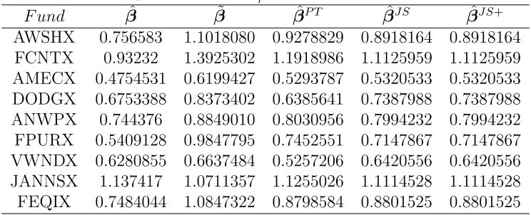
Table 2.3: Estimators ofβ for nine diversified funds
F und βˆ β˜ βˆP T βˆJ S βˆJ S+
AWSHX 0.756583 1.1018080 0.9278829 0.8918164 0.8918164 FCNTX 0.93232 1.3925302 1.1918986 1.1125959 1.1125959 AMECX 0.4754531 0.6199427 0.5293787 0.5320533 0.5320533 DODGX 0.6753388 0.8373402 0.6385641 0.7387988 0.7387988 ANWPX 0.744376 0.8849010 0.8030956 0.7994232 0.7994232 FPURX 0.5409128 0.9847795 0.7452551 0.7147867 0.7147867 VWNDX 0.6280855 0.6637484 0.5257206 0.6420556 0.6420556 JANNSX 1.137417 1.0711357 1.1255026 1.1114528 1.1114528 FEQIX 0.7484044 1.0847322 0.8798584 0.8801525 0.8801525
Let the (S&P) index be a predictor variable, then we can construct the simple
linear multivariate regression model as model (2.1). We consider the data from the
first 10 years (1977-1986) to find the average of the asset’s return as our preliminary
information, which gives the following result:
θ0 = (6.0060,−0.9894,8.2210,1.3112,8.1563,8.0703,11.9730,7.2887,10.3300)0.
Usingθ0 as prior information, we estimate the systematic risks of β using suggested
estimation strategies. The point estimation of the proposed estimators are presented
in Table 2.3. We calculate the risk of the listed estimators, based on 1000 replicates
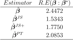
from bootstrapping. We obtain the efficiency of estimators relative to ˆβ; the results
are given in Table 2.4, which are in agreement with the findings of our theoretical
2.6 Concluding Remarks 28
Table 2.4: The relative efficiency of estimators Estimator R.E( ˆβ:β∗)
˜
β 2.4472 ˆ
βJ S 1.5343
ˆ
βJ S+ 1.7750 ˆ
βP T 2.0853
2.6
Concluding Remarks
For a simple multivariate regression model that includes basic investment models,
we have considered various estimation strategies based on a pretest and shrinkage
estimation. In conclusion, the positive-part shrinkage estimator dominates the usual
shrinkage estimator uniformly. Both shrinkage estimators perform well relative to the
usual unrestricted least squares estimator in a wider range that the pretest
estima-tor. The subspace candidate least squares estimator depends heavily on the quality
of the subspace information. The ADR of the restricted least squares estimator is
unbounded when the parameter moves far from the subspace of the restriction, while
the pretest estimator provides good control on the magnitude of the ADR. It is
ex-ceedingly important to note that the shrinkage estimators have the smallest possible
risk in most cases, as compared to other estimators except when the subspace
infor-mation is nearly correct. Further, the application of shrinkage estimators are subject
to the condition that q≥3, where q is the number of parameters in the unrestricted
parameter vector.
The theoretical results in the chapter were verified based on a Monte Carlo
sim-ulation. Indeed, the simulation study shows that the method suggested has sound
2.7 Appendix: Proof of Main Results 29
consistent with findings of the analytical and simulation results.
2.7
Appendix: Proof of Main Results
The following lemma is listed in Sclove et al. (1972), and is used to prove the theorem
in this chapter.
Lemma 2.7.1. Letybe a q-dimensional normal vector distributed asNq(µy,Iq).
Then, for a measurable function of φ, we have
E[yφ(y0y)] = µyE[φ(χ2q+2(∆))]
E[yy0φ(y0y)] = IqE[φ(χq2+2(∆))] +µyµ0yE[φ(χ2q+4(∆))],
where ∆ =µ0yµy
2.7.1
Proof of Theorem 2.4.2
Since ν1,ν2, and ν3 are asymptotically normal, the joint distribution of (ν1,ν2) and
(ν2,ν3) will be asymptotically normal as well.
E(ν2) = lim
n→∞E[n
1/2
( ˜β−β)]}
= lim
n→∞E[n
1/2( ˆβ+C(Hθˆ−h)−β)] underL
n
= 0 + lim
n→∞E[n
1/2C(Hθˆ−h)]
= Cξ
2.7 Appendix: Proof of Main Results 30
Cov(ν2) = Cov( ˜β−β)
= Cov( ˆβ+C(Hθˆ−h)−β)
= Cov( ˆβ) +Cov(C(Hθˆ−h))−2Cov( ˆβ,C(Hθˆ−h))
= Q−01V + (1 + x¯
2
Q0
)CHV H0C0−2¯xQ−01CHV
= Σ∗
E(ν2) = lim
n→∞E[n
1/2( ˜β−β)]}
= lim
n→∞E[n
1/2
( ˆβ+C(Hθˆ−h)−β)] under Ln
= 0 + lim
n→∞E[n
1/2C(Hθˆ−h)]
= Cξ
= γ
E(ν3) = E(ν1−ν2)
= lim
n→∞E[n
1/2( ˆβ−β˜)]
= lim
n→∞E{n
1/2
[−C(Hθˆ−h)]} under Ln
= −Cξ
= −γ
Cov(ν3) = Cov(ν1−ν2)
= Cov(ν1) +Cov(ν2)−2Cov(ν1,ν2)
= Q−01V +Q−01V + (1 + x¯
2
Q0
)CHV H0C0 −2¯xQ−01CHV
− 2Q−01V + 2¯xQ−01CHV
= (1 + x¯
2
Q0
)CHV H0C0
2.7 Appendix: Proof of Main Results 31
2.7.2
Proof of Theorem 2.4.3
In this section we explicitly present a proof of Theorem 2.4.3. Clearly the ADB of ˜β
is equal toγ.
ADB( ˆβP T) = lim
n→∞
√
nE( ˆβP T −β)
= lim
n→∞
√
nE( ˆβ−( ˆβ−β˜)I(P ≤χ2q,α)−β)
= lim
n→∞E[ν1−ν3I(P ≤χ
2
q,α)]
= γHq+2(χ2q(α),∆),
ADB( ˆβJ S) = lim
n→∞
√
nE( ˜β+ (1−mP−1)( ˆβ−β˜)−β)
= lim
n→∞E(ν1−mν3P −1)
= mγE(χ−q+22 (∆)),
ADB( ˆβJ S+) = lim
n→∞
√
nE{( ˆβJ S−β)−(1−mP−1)( ˆβ−β˜)I(P < m)}
= ADB( ˆβJ S)−γE{(mχq−+22 (∆)−1)I(χ2q+2(∆) < m)}.
2.7.3
Proof of Theorem 2.4.4
Clearly the AM SE( ˜β) is equal to Σ∗+γγ0. AM SE( ˆβP T) can be written as
= lim
n→∞E{n( ˆβ
P T −β)( ˆβP T −β)0}
= lim
n→∞E{[ν1−ν3I(P < χ
2
q(α))][ν1−ν3I(P < χ2q(α))]
0}
= lim
n→∞E{ν1ν1 0−
2.7 Appendix: Proof of Main Results 32
Note that, by using Theorem 2.4.2 and Lemma 2.7.1, for E(ν3ν10I(P < χ2q(α))) we
have
= E(E(ν3ν10I(P < χ2q(α))|ν3))
= E(ν3[E(ν1) +Ω21Ω∗−1(ν3−E(ν3))]0I(P < χ2q(α)))
= Ω12Hq+2(χ2q(α),∆) +γγ
0
Ω∗−1Ω12[Hq+4(χ2q(α),∆) +Hq+2(χ2q(α),∆)].
Therefore,
AM SE( ˆβP T) = Q−01V −2{Ω12Hq+2(χ2q(α),∆) +γγ
0
Ω∗−1Ω12[Hq+4(χ2q(α),∆) +
Hq+2(χ2q(α),∆)]}+Ω
∗
Hq+2(χ2q(α),∆) +γγ
0
Hq+4(χ2q(α),∆)
AM SE( ˆβJ S) = lim
n→∞E{n[( ˆβ−β)−mP
−1( ˆβ−β˜)][( ˆβ−β)−mP−1( ˆβ−β˜)]0}
= V ar(ν1) +E(ν1)E(ν1)0−2E(ν3ν10mP−1) +E(ν3ν30(mP−1)2).
Note that, by using Theorem 2.4.2 and Lemma 2.7.1, we have
E(ν3ν10P−1) = E(E(ν3ν10P−1|ν3))
= E(ν3[E(ν1) +Ω21Ω∗−1(ν3−E(ν3))]0P−1)
= E(ν3ν30Ω∗−1Ω12P−1+ν3γ0Ω∗−1Ω12P−1)
= Ω12E(χ−q+22 (∆)) +γγ
0
Ω∗−1Ω12[E(χ−q+42 (∆)) +E(χ
−2
q+2(∆))].
Therefore,
AM SE( ˆβJ S) = Q−01V −2m{Ω12E(χ−q+22 (∆)) +γγ
0
Ω∗−1Ω12[E(χ−q+42 (∆)) +
2.7 Appendix: Proof of Main Results 33
We got the result after some computation. Similarly,
AM SE( ˆβJ S+) = lim
n→∞E{n[( ˆβ
J S−β)−(1−mP−1)( ˆβ−β˜)I(P < m)]
× [( ˆβJ S−β)−(1−mP−1)( ˆβ−β˜)I(P < m)]0}
= AM SE( ˆβJ S)
− 2 lim
n→∞nE{( ˆβ− ˜
β)( ˆβJ S−β)0(1−mP−1)I(P < m)}
+ lim
n→∞nE[( ˆβ− ˜
β)( ˆβ−β˜)0(1−mP−1)2I(P < m)].
Note that by using the definition of ˆβJ S from Section 2.3 in the second term of the
above equation and substituting ˜β−β= ˜β−βˆ+ ˆβ−β, we have
− 2 lim
n→∞nE{( ˆβ− ˜
β)[( ˜β−β) + (1−mP−1)( ˆβ−β˜)]0 ×(1−mP−1)I(P < m)}=
− 2 lim
n→∞nE{( ˆβ− ˜
β)( ˆβ−β)0(1−mP−1)I(P < m)} (1*)
+ 2 lim
n→∞nE{( ˆβ− ˜
β)( ˆβ−β˜)0(1−mP−1)I(P < m)} (2*)
− 2 lim
n→∞nE{( ˆβ− ˜
β)( ˆβ−β˜)0(1−mP−1)2I(P < m)} (3*).
Now, by substituting ˆβ−β = ˆβ−β˜+ ˜β−β in (1∗),we get
(1∗) = − 2 lim
n→∞nE{( ˆβ− ˜
β)( ˆβ−β˜)0(1−mP−1)I(P < m)} same as (2∗)
− 2 lim
n→∞nE{( ˆβ− ˜
β)( ˜β−β)0(1−mP−1)I(P < m)}.
Therefore, the second term in AM SE( ˆβJ S+) will be simplified as follows:
−2 lim
n→∞E[ν3ν2 0
(1−mP−1)I(P < m)]−2 lim
n→∞E[ν3ν3 0
2.7 Appendix: Proof of Main Results 34
As well the third term in AM SE( ˆβJ S+) will be simplified as
= E[ν3ν30(1−mP−1)2I(P < m)]
= Ω∗E(1−mχ−q+22 (∆))2I(χ2q+2(∆)< m) +γγ0E(1−mχ−q+42 (∆))2I(χ2q+4(∆)< m).
Finally, by using Theorem 2.4.2 and Lemma 2.7.1, the AMSE of a positive shrinkage
estimator is
= AM SE( ˆβJ S)−Ω∗E(1−mχ−q+22 (∆))2I(χ2q+2(∆)< m)
+ 2γγ0E(1−mχ−q+22 (∆))I(χ2q+2(∆)< m)−γγ0E(1−mχ−q+42 (∆))2I(χ2q+4(∆)< m).
2.7.4
Proof of Theorem 2.4.5
In an effort to prove Theorem 2.4.5, we need to show some useful preliminary results.
Clearly, the asymptotic risk of ˆβ is equal to tr(WQ−01V) = Q−01tr(W V). Also, we
get the following expression for the asymptotic risk of ˜β:
ADR( ˜β;W) = Q0−1tr(W V) +a×tr(W CHV H0C0)−2b×tr(W CHV) +γ0W γ.
Since the risk of ˜βdepends onγ0W γ, whereγ =Cξ, note thatV−12CHV H0C0V− 1 2
2.7 Appendix: Proof of Main Results 35
matrix Γ such that
ΓV−12CHV H0C0V− 1 2Γ0 =
Iq 0
0 0
ΓV 12W V 1 2Γ0 =
Z11 Z12
Z21 Z22
.
We need to show that
tr[W CHV H0C0] = tr[{ΓV 12W V 1
2Γ0} × {ΓV−
1
2CHV H0C0V− 1 2Γ0}]
= tr[
Z11 Z12
Z21 Z22
Iq 0
0 0
] =tr(Z11),
and we may write
γ0W γ = ξ0C0W Cξ
= ξ0{ΓV−12CHV H0C0V− 1
2Γ0}{ΓV 1 2W V
1 2Γ0}
{ΓV−12CHV H0C0V− 1 2Γ0}ξ
= η0
Iq 0
0 0
Z11 Z12
Z21 Z22
Iq 0
0 0
η =η
0
1Z11η1,
where η=ΓV−12CHV H0ξ =
η1 η2
. Therefore,
2.7 Appendix: Proof of Main Results 36
Similarly forADR( ˆβP T;W) we have
= Q−01tr(W V) + [tr(W G)−2tr(W F)]Hq+2(χ2q(α),∆)
− 2tr(W γγ0A)(Hq+2(χ2q(α),∆) +Hq+4(χq2(α),∆)) +tr(W γγ
0
)Hq+4(χ2q(α),∆))
= Q−01tr(W V) + [a×tr(Z11)−2b×tr(W CHV)]Hq+2(χ2q(α),∆)
− 2tr(W γγ0A)[Hq+2(χ2q(α),∆) +Hq+4(χ2q(α),∆)] +η
0
1Z11η1Hq+4(χ2q(α),∆)).
Finally, for ADR( ˆβJ S;W) we have
= Q−01tr(W V)−2m{tr(W F)E(χ−q+22 (∆))
− tr(W γγ0A)[E(χq−+42 (∆)) +E(χ−q+22 (∆))]}
+ m2[tr(W G)E(χq−+24 (∆)) +tr(W γγ0)E(χ−q+44 (∆))]
= Q−01tr(W V)−2mb×tr(W CHV)E(χ−q+22 (∆))
− 2m×tr(W γγ0A)[E(χq−+42 (∆)) +E(χ−q+22 (∆))]
+ am2×tr(Z11)E(χ−q+24 (∆)) +m2×η
0
1Z11η1E(χ−q+44 (∆))],
and similarly for ADR( ˆβJ S+;W) we have
= ADR( ˆβJ S)−tr(W G)[E(1−mχq−+22 (∆))2I(χ2q+2(∆) < m)]
+ tr(W γγ0){2E(1−mχ−q+22 (∆))I(χ2q+2(∆)< m)
− E(1−mχ−q+42 (∆))2I(χ2q+4(∆)< m)}
= ADR( ˆβJ S)−a×tr(Z11)[E(1−mχ−q+22 (∆))
2I(χ2
q+2(∆) < m)]
+ η10Z11η1{2E(1−mχ−q+22 (∆))I(χ 2
q+2(∆) < m)
Chapter 3
Estimation Strategies for a
Parameter Matrix in a
Multivariate Regression Model
.
3.1
Introduction
In many areas of scientific research, the basic goal is to assess the simultaneous
in-fluence of several covariates on the response variable, and the quantity of interest.
Multiple regression models provide an extremely powerful methodology to achieve
this task. The multivariate multiple regression model (MMRM) generalizes the
mul-tiple regression model for the prediction of several response variables from the same
set of explanatory variables. A common example of multivariate responses occur in