Parameter Estimation of Nonlinear System - VanderPol Oscillator using Neural Networks

(1)

Copyright to IJIRCCE DOI: 10.15680/IJIRCCE.2017. 0506078 11436

Parameter Estimation of Nonlinear System -

VanderPol Oscillator using Neural Networks

Yugchhaya Dhote

Assistant Professor, Dept. of Computer Engineering, VESIT, Mumbai University, Mumbai, India

ABSTRACT: The problem of system modeling and identification has attracted considerable attention during the past decades because of a large number of applications in diverse fields. The modeling and identification of linear and nonlinear system through the use of measured experimental data is a problem of considerable importance in engineering. Models of real system are of fundamental importance in virtually all the disciplines. Models can be useful for system analysis i.e. for gaining a better understanding of the system. Models make it better understanding of the system.. In this light, the paper presents objective of the present work was to develop a neural network scheme for identification and parameter estimation of various types of nonlinearities. The identification procedure is based on Neural Network concepts involving back-propagation algorithm

KEYWORDS: Nonlinear systems, System Identification, Artificial neural network, Back propagation Algorithm, Vanderpol Oscillator,

I. INTRODUCTION

Inverse problems of system identification and parameter estimation are crucial in nonlinear analysis. Response behaviour of nonlinear systems under specific excitation can be only predicted accurately when the system structure and the parameters are completely known. System identification is the task of a inferring a mathematical description of a dynamic system from a series of measurement on the system. A mathematical description of this kind is called a model of the system. There are two ways in which a model can be established: it can be derived using laws of nature, or it can be inferred from a set of data collected during a practical experiment with the system. The first method looks simple but it is very difficult to use them in real situations. The second method which is commonly referred to as system identification, in these situation can be useful for deriving the mathematical models

While sufficient literature is available on system identification in general, most of this deals with systems described by linear differential equations or difference equations. However, motivated by the fact that almost all real systems exhibit some kind of nonlinear behaviour, lately there have been serious efforts on different approaches to nonlinear system identification.

One of the key approaches towards identification in engineering systems has been Artificial Neural Network (ANN). An artificial neural network operates by creating connections between many different processing elements, each analogous to a single neuron in a biological brain. These neurons may be physically constructed or simulated by a digital computer. Each neuron takes many input signals, then, based on an internal weighting system, and produces a single output signal that's typically sent as input to another neuron. The neurons are tightly interconnected and organized into different layers. The input layer receives the input; the output layer produces the final output. Usually one or more hidden layers are sandwiched in between the two. This structure makes it impossible to predict or know the exact flow of data.

II. RELATED WORK

(2)

nonlinear systems. This was subsequently followed by identification of nonlinear system with multiple degrees of freedom by Chassiakos et.al[7].

Kosmatopoulos et al[8] and Pei et al.[9] presented a procedure for identification of nonlinear hysteretic dynamic system which used a static neural network module in conjunction with dynamic linear module. Subsequently Le Riche et.al.[10] and Song et al.[11] suggested that the neural network does not learn the function showing the relationship between input and output but learns the relationship that links system features and its parameters. Liang et al. [12] further investigated fuzzy adaptive neural networks with increased network training speed. Fan et.al [13] developed a hybrid approach embedding neural networks in a physical model to represent unknown nonlinearities. This was followed by a related study using radial basis function network by Saadat et al[14].

In addition to use of neural network as one of the tool for black box modeling of non linear systems, a lot of alternative approaches have been developed and extensively cited in nonlinear system identification literature.

Earliest work on bypassing nonlinearity was proposed by Caughey [15][16][17] which involved replacing a nonlinear system with a given excitation by an equivalent linearized system with same excitation. The common statistical criterion used for bypassing non linearity is that the means square error (MSE) between the real life nonlinear system and its equivalent linearized system is kept to a minimum level. This subsequently lead to many advancements (Iwan et.al [18][19] and Roberts et.al[20]) in the field, however it has been observed that equivalent linearization method of strongly nonlinear system fails to predict the response to an acceptable accuracy.

Data which is considered during the identification process using Time domain approach is in the form of time series. Such techniques have the distinct advantage that the signals are directly provided by measurement devices and data processing can be accomplished in minimal time, Masri et.al [21] introduced the restoring force approach to time series identification. A parallel approach using forced state mapping was introduced by Crawley et.al [22][23]. The method were initially developed for SDOF but were soon developed for MDOF systems as well by Masri et.al [24]. Many alternative time-domain techniques have been proposed in the literature.

The identification process in Frequency-domain methods takes the form of FRFs or spectra. The method for nonlinear system identification using frequency-domain was initially proposed by Yasuda et.al [25] which analyzed the systems with steady state response with external excitation. This was extended to chaotic systems by Yuan et.al [26] and for MDOF by Liang et.al [27]

Modal analysis is undoubtedly the most popular approach to linear system identification and have been explored in detail by Heylen et al [28], Maia et.al [29], Ewins et.al[30]. In case of nonlinear systems, modal analysis is based on assumption of weak nonlinearities.

III. PROPOSED WORK

A. Introduction:

Parameter estimation is the final step towards establishment of model with a good predictive accuracy. An important condition which affects the success of parameter estimation is that all the nonlinearities throughout the systems have been properly characterised.

Several methods have been established methods for parameter estimation. Some of which are mentioned below: o The restoring force surface method.

o Direct parameter estimation.

o Auto regressive and NARMAX modeling. o The Hilbert transform.

o The Volterra series. o Feedback of output. o Nonlinear resonant decay.

(3)

1) VanderPol Oscillator

2

(1

)

( )

x

d x

x

f t

t



d t











(eq.1)

It represents non-conservative system in which energy is added to and subtracted from the system in an autonomous fashion, resulting in a periodic motion called a limit cycle. Here we can see that the sign of the damping term, changes, depending upon whether |x| is larger or smaller than unity. VanderPol’s equation has been used as a model for stick-slip oscillations, aero-elastic, flutter, and numerous biological oscillators, to name but a few of its applications.

The restoring function is of the form of

2

(

,

)

(

1 )

f

x y





x



y



x

(eq. 2)

This system corresponds to the homogenous VanderPol equation which is used to model several mechanical and electrical systems.

B. Proposed Neural Network Architecture:

Since there are no set procedure to arrive at the topology, extensive experimentation was carried out with different topologies to arrive the best possible network. A single hidden layer is generally sufficient to represent a variety of continuous function.

The Network topology finally found to best suit the given data was:

Number of inputs =2 (displacement and velocity) Number of outputs=1 (restoring force)

Number of hidden layer=1 Number of hidden neurons =16 Activation function:

Hidden layer = logsig Output layer = purelin

Algorithm: Levenberg Marquardt.

Estimation method: Restoring Force surface Method Sampling time

(4)

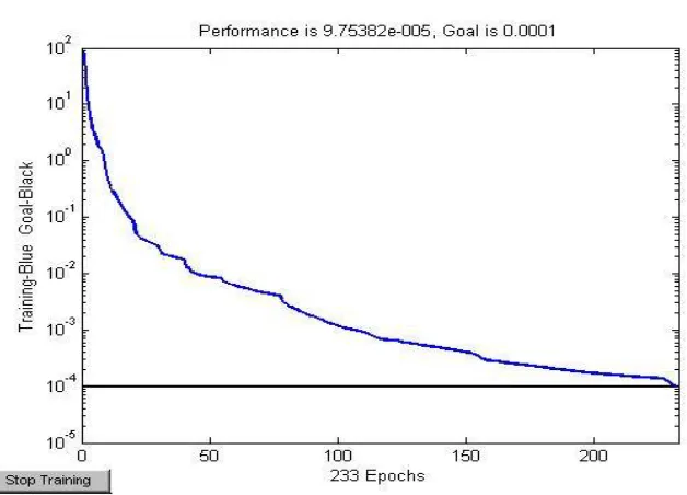
Fig 1 Convergence of network during training phase

C. Data set Generation for Training and Validation

The response x and y of equation (1) is numerically simulated for the following data with



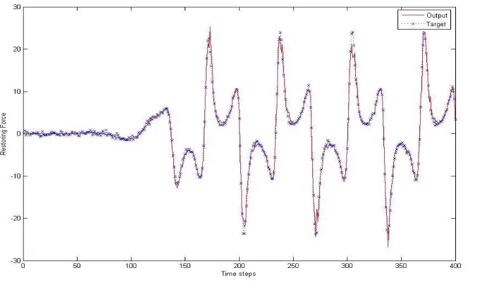
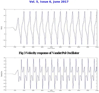
=0.2, initial condition vector. The response is shown in Figs. (2) and (3) and form the input to the neural network. The expected output as shown in Fig (4) is the restoring force f (x , y).

(5)

Fig 3 Velocity response of VanderPol Oscillator

Fig 4 Restoring Force response of VanderPol Oscillator

A three-layer feed forward neural network is trained using back propagation algorithm. Levenberg Marquardt algorithm was chosen as training algorithm. This was chosen after extensive experimentation with various algorithms the result of which is shown in Table 1.

Table 1: Comparison of various Learning Algorithms

Sr no.

Algorithms No. of

Epochs

Means square error(10-3)

1. Variable learning rate 500 16.45

2. Variable learning rate with momentum 500 14.61

3. Resilient back propagation 500 6.39

4. Fletcher Reeves Update 500 5.83

5. Polak-Ribiere Update 500 3.67

6. Quasi Newton algorithm 500 0.020261

(6)

All algorithms were tested with same training data with same initialization of weights.

D. Neural Network Training and Validation

Effect of change in initial conditions and parameters on the network performance was examined.

(a) The initial condition: Input data were generated by numerical simulation of VanderPol equation with following sets of new initial conditions.

(a)

The initial condition: Input data [

x y

,

] were generated by numerical simulation of VanderPol equation with following sets of new initial conditions.



x

1

(0),

y

1

(0)

 

 

0.01, 0.01







x

2

(0),

y

2

(0)

 

 

0.1, 0.1





x

3

(0),

y

3

(0)

 



0.1, 0.5





Network response for various pairs of initial conditions is shown in Fig.5.

(a)



x

1

(0),

y

1

(0)

 

 

0.01, 0.01





MSE=0.00467

(7)

(c)



x

3

(0),

y

3

(0)

 



0.1, 0.5





MSE=0.00121

Fig 5 Effect of Initial Conditions on Network performance

These data corresponding to various new sets of

[ (0), (0)]

x

y

were given as an input to network, which was trained

with data corresponding to

[ (0), (0)]

x

y



[0.01, 0.01]

. The network was tested for different sets of initial conditions. Network is seen quite robust to change in initial condition.

(b)

Effect of parameter



: Changing



is expected to have a greater effect on network prediction ability. Since a

large



produces responses (

x

,

y

) out of range of values used during training. Fig. 6 shows the network performance

when data generated using various values of



was fed to network previously trained using data corresponding to value

of





0.2

.

(8)

(b)



=0.17 MSE=10.120

(c)



=0.205 MSE=0.1350

(d)



=0.23 MSE=2.8449

(9)

It is seen that the network when fed by the data other than



=0.2, now missing the peaks, since it has been never trained for that range of values. The behaviour of the performance can be observed can be shown in Fig.7.



Fig 7 Variation of MSE w.r.t.



(c)

Effect of noise: Network performance was tested in presence of noise. The network trained on noiseless data was tested with a data with additive white noise of power 0.01, the network performed satisfactorily with a MSE of 1.2523.

.

Fig 8 Effect of noise on network performance

(10)

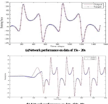
(a)Network performance on data of 15s – 20s

(b) Network performance on data of 0s -10s Fig 9 Effect of sampling period on network performance

(e)

Effect of sampling time: Network performance was tested using data collected using different sampling times of

t



_{=0.05s and}



t

_{=0.2s. The performance of network was seen unaffected by change in sampling time.}

(11)

(b)



t

=0.2s MSE = 1.4960e-004

Fig.10 Effect of sampling time



t

on network performance for VanderPol Oscillator

(f)

Effect of length of training set: Effect of length of training set was studied on the network performance. The network was trained with different length of data set. Not much effect of length of training set was found on the network performance

IV. CONCLUSION AND FUTURE WORK

During parameter estimation of Vanderpol Oscillator it was observed that the neural network models developed were quite robust to change in initial conditions, sampling time, sampling period, and length of training set. However it was observed that a substantial change in nonlinear stiffness term has a considerable effect on the network performance of VanderPol Oscillator. The network models were tested in presence of noise and it was observed that the network was quite robust to noise. Though only VanderPol was considered for identification stage, the same procedure can be applied for identification and classification of other non-linear systems also. In present study, the emphasis was on identification and parameter estimation of single-degree of freedom. Future work can be directed towards multi-degree of freedom system

REFERENCES

1. S.R. Chu, R. Shoureshi, M. Tenorio, Neural networks for system identification, IEEE Control Systems Magazine 10 (1990) 36–43.

2. K.S. Narendra, K. Parthasarathy, Identification and control of dynamical systems using neural networks, IEEE Transactions on Neural Networks 1 (1990) 4–27.

3. S.A. Billings, H.B. Jamaluddin, S. Chen, Properties of neural networks with applications to modelling non-linear dynamical systems, International Journal of Control 55 (1991) 193–224.

4. S. Chen, S.A. Billings, C.F.N. Cowan, P.M. Grant, Nonlinear-systems identification using radial basis functions, International Journal of Systems Science 21 (1990) 2513–2539.

5. K. Worden, G.R. Tomlinson, Modelling and classification of nonlinear systems using neural networks—I simulation, Mechanical Systems and Signal Processing 8 (1994) 319–356.

6. K. Worden, G.R. Tomlinson, W. Lim, G. Sauer, Modelling and classification of non-linear systems using neural networks—II: a preliminary experiment, Mechanical Systems and Signal Processing 8 (1994) 395–419

7. A.G. Chassiakos, S.F. Masri, Modelling unknown structural systems through the use of neural networks, Earthquake Engineering and Structural Dynamics 25 (1996) 117–128.

8. E.B. Kosmatopoulos, A.W. Smyth, S.F. Masri, A.G. Chassiakos, Robust adaptive neural estimation of restoring forces in nonlinear structures, Journal of Applied Mechanics 68 (2001) 880–893.

(12)

10. R. Le Riche, D. Gualandris, J.J. Thomas, F.M. Hemez, Neural identification of non-linear dynamic structures, Journal of Sound and Vibration 248 (2001) 247–265.

11. Y. Song, C.J. Hartwigsen, D.M. McFarland, A.F. Vakakis, L.A. Bergman, Simulation of dynamics of beam structures with bolted joints using adjusted Iwan beam elements, Journal of Sound and Vibration 273 (2004) 249–276.

12. Y.C. Liang, D.P. Feng, J.E. Cooper, Identification of restoring forces in non-linear vibration systems using fuzzy adaptive neural networks, Journal of Sound and Vibration 242 (2001) 47–58.

13. Y. Fan, C.J. Li, Non-linear system identification using lumped parameter models with embedded feedforward neural networks, Mechanical Systems and Signal Processing 16 (2002) 357–372.

14. S. Saadat, G.D. Buckner, T. Furukawa, M.N. Noori, An intelligent parameter varying approach for non-linear system identification of base excited structures, International Journal of Non-Linear Mechanics 39 (2004) 993–1004.

15. T.K. Caughey, Response of Van der Pol’s oscillator to random excitations, Journal of Applied Mechanics 26 (1959) 345–348. 16. T.K. Caughey, Random excitation of a system with bilinear hysteresis, Journal of Applied Mechanics 27 (1960) 649–652. 17. T.K. Caughey, Equivalent linearisation techniques, Journal of the Acoustical Society of America 35 (1963) 1706–1711.

18. W.D. Iwan, A generalization of the concept of equivalent linearization, International Journal of Non-Linear Mechanics 8 (1973) 279–287. 19. W.D. Iwan, A.B. Mason, Equivalent linearization for systems subjected to non-stationary random excitation, International Journal of Non-linear

Mechanics 15 (1980) 71–82.

20. J.B. Roberts, P.D. Spanos, Random Vibrations and Statistical Linearization, Wiley, New York, 1990.

21. S.F. Masri, T.K. Caughey, A nonparametric identification technique for nonlinear dynamic problems, Journal of Applied Mechanics 46 (1979) 433–447.

22. E.F. Crawley, K.J. O’Donnell, Identification of nonlinear system parameters in joints using the force-state mapping technique,AIAA Paper 86-1013 (1986) 659–667

23. E.F. Crawley, A.C. Aubert, Identification of nonlinear structural elements by force-state mapping, AIAA Journal 24 (1986) 155–162.

24. S.F. Masri, H. Sassi, T.K. Caughey, A nonparametric identification of nearly arbitrary nonlinear systems, Journal of Applied Mechanics 49 (1982) 619–628.

25. K. Yasuda, K. Kamiya, Experimental identification technique of vibrating structures with geometrical nonlinearity, Journal of Applied Mechanics 64 (1997) 275–280.

26. C.M. Yuan, B.F. Feeny, Parametric identification of chaotic systems, Journal of Vibration and Control 4 (1998) 405–426.

27. Y. Liang, B.F. Feeny, Parametric identification of chaotic base-excited double pendulum experiment, ASME International Mechanical Engineering Congress, Anaheim, 2004.

28. W. Heylen, S. Lammens, P. Sas, Modal Analysis Theory and Testing, KUL Press, Leuven, 1997.

29. N.M.M. Maia, J.M.M. Silva, Theoretical and Experimental Modal Analysis, Research Studies Press LTD, Taunton, 1997. 30. D.J. Ewins, Modal Testing: Theory, Practice and Application, second ed., Research Studies Press LTD, Hertfordshire, 2000.

31. of Dynamic Systems, Springer, 2000.

32. Zurada, M.J., Introduction to Artificial Neural Systems, Jaico Publishing House, Delhi, 1999.

BIOGRAPHY