Simulator Designed for Performance
Evaluation of Embedded Real-Time Operating
Systems
Geetika Kesar, Rajesh Garg, Nitika Bansal
Student, Dept. of CSE, Ganpati Institute of Technology and Management, Bilaspur, India
Lecturer, Dept. of ECE, Seth Jai Prakash Polytechnic for Engineering, Damla, India
Assistant Professor, Dept. of CSE, Ganpati Institute of Technology and Management, Bilaspur, India
ABSTRACT: An embedded system is multitasking and consist one or more processing units completely encapsulated
inside the system. They have stringent timing constraints associated with their specification. Performance evaluation approach for embedded system before final implementation on hardware helps to find essential characteristics. Simulation has been adopted as a tool for real-time embedded system software in a stochastic environment. The simulator is used to evaluate and compare the performances of both Preemptive priority scheduling and Non Preemptive scheduling algorithms with the parameters average waiting time and average turnaround time for a number of processes.
KEYWORDS: Embedded Real time operating system, Scheduling Algorithm, Fault Tolerance, Performance
Evaluation.
I. INTRODUCTION
An embedded system is hardware/ software co-design methodology, to perform specific task [1]. Most of the embedded systems are the real time where all tasks must execute within their timing constraints even in the presence of faults. Embedded Systems are used everywhere, Millions of embedded systems build every year for different purposes, 98% computing devices in the world are embedded systems. Safety-critical embedded systems have to satisfy cost and performance constraints even in the presence of faults. When the use of fault-tolerant real-time embedded systems, we tried to integrate fault tolerance techniques and task scheduling. Reliability requirement in safety-critical embedded system can be achieved by fault tolerance techniques. Scheduling is the process of selecting the next request [2]. Designing of Real-time embedded system is always a challenging task. To evaluate system performance before implementation on hardware is also most challenging task. Some research work has been done to address this problem. The problem becomes even more complex with RTS because not all RTS use RTOS [6] so designers now have to spend a lot of time to study different implementations before choosing the right design for the target application. In this paper, we tackle the performance evaluation problem and explore different methods to evaluate the performance. We are extending the work done in [4] and present a comparative analysis of two different techniques that evaluate the performance based on the parameters average waiting time and average turnaround time. The system compares the performances of both scheduling algorithms and finds out the best for designing of embedded real-time operating System.
II. DESIGN OF SIMULATOR
and non preemptive gives intermediate wait and turnaround time. The burst time is generated using exponential distribution with the average burst rate of 6.5. The same distribution is used to generate processes arrival time but with inter-arrival rate 5. The priority of the process is generated using rand() and substituting this value into exponential distribution in place of mean arrival and mean burst. The total number of processes is entered by the user and the scheduling algorithm is implemented by calling the respective function. The final results are then displayed to the user. Simulator has been designed for one type of scheduling i.e. Priority scheduling. Two types of priority scheduling: Preemptive and Non-preemptive.
Algorithm 1: Simulation Design Main
Step-1: Input the total no. processes from user.
Read Number of Processes in variable PROCESS
Step-2: Simulate preemptive scheduling.
Call Preemptive_Sch (PROCESS,CART[],BT[],Priority[])
Step-3: Simulate non-preemptive scheduling.
Call Non_Preemptive_Sch(PROCESS,CART[],BT[],Priority[])
Step-4: Display the output.
Algorithm 2: Preemptive_Sch (PROCESS, CART [], BT[], Priority [])
Step-1: [Initialization]
TotalWaitingTime = 0 AvgWaitingTime = 0
TotalTurnaroundTime = 0 AvgTurnaroundTime = 0 Count = 0
BtSum= 0 Time = 0
Step-2: [Read the process workload on the system from disk file(s) in integer variable PROCESS]
Step-3: Repeat for count =0 to Process-1
BtSum = BtSum + Burst (count) [end of step (3) loop]
Step-4: [Initialize the variable inCPU to the current value of count variable that hold the total number of
processes]
inCPU = count
Step-5: Repeat for time = 0 to BtSum
Step-6: Repeat for i = 0 to PROCESS-1
IF CART(i) <= time AND Priority(i)< Priority(inCPU) THEN Set inCPU = i
[end of IF] [end of step (6) loop]
Step-7:[Decrement TimeRemaining array by 1 for inCPU counter, TimeRemaining is the array that holds the
service time left for the processes]
TimeRemaining(inCPU)= TimeRemaining(inCPU)-1
Step-8: IF TimeRemaining(inCPU) = 0 THEN
Set FinishTime(inCPU) = time+1 inCPU = inCPU-1
[end of IF] [end of step(5) loop]
Step-9: Repeat for i = 0 to PROCESS-1
Set WaitingTime(i) = FnishTime() – Burst(i) – CAT(i) TurnaroundTime(i) = WaitingTime(i) + Burst(i) [end of step(9) loop]
Repeat for i = 0 to PROCESS-1
CumulativeWaitingTime=CumulativeWaitingTime+WaitingTime() CumulativeTurnaroundTime=CumulativeTurnaroundTime+
TurnaroundTime(i) [end of step(10) loop]
Step-11: [Compute the Average waiting time and average turnaround time]
AvgWaitingTime = CumulativeWaitingTime/PROCESS
AvgTurnaroundTime = CumulativeTurnaroundTime/PROCESS
Step-12: End.
Algorithm 3: Non-Preemptive_Sch (PROCESS, CART[], BT[], Priority[])
Step-1: [Initialization]
TotalWaitingTime = 0, AvgWaitingTime = 0, TotalTurnaroundTime = 0,
AvgTurnaroundTime = 0,
Count = 0, BtSum = 0, Time = 0
Step-2: [Read the process workload on the system from disk file(s) in integer variable PROCESS]
Step-3: Repeat for count =0 to Process-1
BtSum = BtSum+Burst(count) [end of step(3) loop]
Step-4: [Initialize the variable inCPU to the current value of count variable that hold the total number of
processes]
inCPU = count
Step-5: Repeat for time = 0 to BtSum
IF time = 0 THEN
Set isIdle = true [isIdle is a Boolean variable] [end of IF]
IF inCPU≠-1 AND time=StartTime(inCPU)+Burst(inCPU) THEN Set IsIdle = true;
FinishTime(inCPU)= Time; [end of IF]
[StartTime and FinishTime are the arrays that hold the starting time and finishing time of all processes that process takes]
Step-6: Repeat for count =0 to Process-1
IF Priority(count)<Priority(inCPU) AND CART(count)<=Time THEN Set StartTime(count) = time
isIdle = false inCPU = count [end of step(6) loop]
[end of step(5) loop]
Step-7: Repeat for i = 0 to PROCESS-1
Set WaitingTime(i) = StartTime() – CART(i) TurnAroundTime(i) = WaitingTime(i) + Burst(i) [end of step(7) loop]
Step-8: [Compute the total waiting time and turnaround time of the all the processes]
Repeat for i = 0 to PROCESS-1
CumulativeWaitingTime = CumulativeWaitingTime + WaitingTime(i) CumulativeTurnaroundTime= CumulativeTurnaroundTime + TurnaroundTime(i) [end of step(8) loop]
AvgWaitingTime = CumulativeWaitingTime/PROCESS AvgTurnaroundTime = CumulativeTurnaroundTime/PROCESS
Step-10: End.
III. RESULT AND DISCUSSION
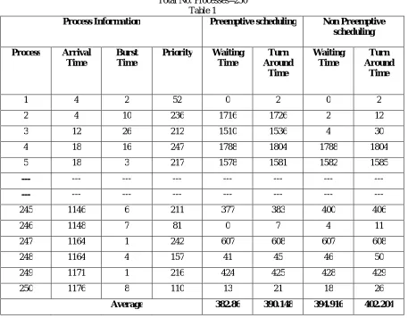
Table 1 shows the no. of processes; burst time, arrival time and priority of 250 processes with their corresponding algorithms Preemptive and Non preemptive with parameters waiting time and turnaround time. The parameters like average waiting time and average turnaround time are measured. The average waiting time for preemptive scheduling is 382.86 ms and average turnaround time is 390.148 ms and average waiting time for non preemptive scheduling is 394.916 ms and average turnaround time is 402.204ms. Table explains about the output of Simulator for different types of scheduling techniques.
Total No. Processes=250 Table 1
Process Information Preemptive scheduling Non Preemptive
scheduling
Process Arrival
Time
Burst Time
Priority Waiting
Time
Turn Around
Time
Waiting Time
Turn Around
Time
1 4 2 52 0 2 0 2
2 4 10 236 1716 1726 2 12
3 12 26 212 1510 1536 4 30
4 18 16 247 1788 1804 1788 1804
5 18 3 217 1578 1581 1582 1585
--- --- --- --- --- --- --- ---
--- --- --- --- --- --- --- ---
245 1146 6 211 377 383 400 406
246 1148 7 81 0 7 4 11
247 1164 1 242 607 608 607 608
248 1164 4 157 41 45 46 50
249 1171 1 216 424 425 428 429
250 1176 8 110 13 21 18 26
Average 382.86 390.148 394.916 402.204
Table 2 shows the no. of processes; burst time, arrival time and priority of 750 processes with their corresponding algorithms Preemptive and Non preemptive with parameters waiting time and turnaround time. The average waiting time for preemptive scheduling is 1001.66ms and average turnaround time is 1008.69ms and average waiting time for non preemptive scheduling is 1018.3 ms and average turnaround time is 1025.34 ms.
Process Information Preemptive scheduling
Non Preemptive scheduling
Process Arrival
Time
Burst Time
Priority Waiting
Time
Turn Around
Time
Waiting Time
Turn Around
Time
1 3 1 584 0 1 0 1
2 5 3 430 17 20 17 20
3 5 14 42 0 14 0 14
4 13 1 190 6 7 6 7
5 20 2 317 0 2 0 2
--- --- --- --- --- --- --- ---
--- --- --- --- --- --- --- ---
745 3391 4 160 10 14 21 25
746 3391 12 445 89 101 90 102
747 3391 3 480 209 212 209 212
748 3394 3 529 520 523 526 529
749 3395 3 419 52 55 53 56
750 3396 8 447 96 104 97 105
Average 1001.66 1008.69 1018.3 1025.34
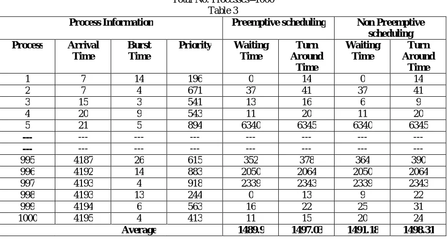
Table 3 shows the no. of processes; burst time, arrival time and priority of 1000 processes with their corresponding algorithms Preemptive and non preemptive with parameters waiting time and turnaround time. The parameter like average waiting time and average turnaround time are measured. The average waiting time for preemptive scheduling is 1489.9ms and average turnaround time is 1497.03ms and average waiting time for non preemptive scheduling is 1491.18ms and average turnaround time is 1498.31ms.
Total No. Processes=1000 Table 3
Process Information Preemptive scheduling Non Preemptive
scheduling
Process Arrival
Time
Burst Time
Priority Waiting
Time
Turn Around
Time
Waiting Time
Turn Around
Time
1 7 14 196 0 14 0 14
2 7 4 671 37 41 37 41
3 15 3 541 13 16 6 9
4 20 9 543 11 20 11 20
5 21 5 894 6340 6345 6340 6345
--- --- --- --- --- --- --- ---
--- --- --- --- --- --- --- ---
995 4187 26 615 352 378 364 390
996 4192 14 883 2050 2064 2050 2064
997 4193 4 918 2339 2343 2339 2343
998 4193 13 244 0 13 9 22
999 4194 6 563 16 22 25 31
1000 4195 4 413 11 15 20 24
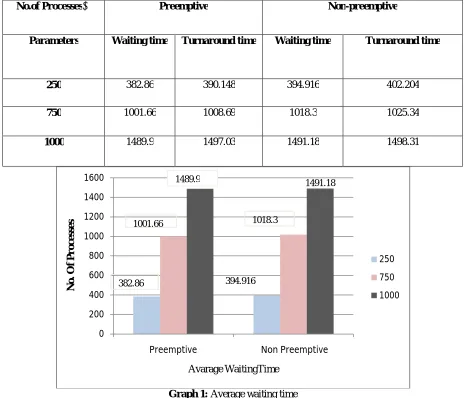
Table 4 represents the comparison of both scheduling algorithms with parameters average waiting time and turnaround time with their corresponding graphs.
Graph1 represent the average waiting time of both scheduling algorithms and Graph 2 represent the average turnaround time.
Table 4: Waiting time and Turnaround time for 250, 750 and 1000 Processes
No.of Processes Preemptive Non-preemptive
Parameters Waiting time Turnaround time Waiting time Turnaround time
250 382.86 390.148 394.916 402.204
750 1001.66 1008.69 1018.3 1025.34
1000 1489.9 1497.03 1491.18 1498.31
Graph 1: Average waiting time
0 200 400 600 800 1000 1200 1400 1600
Preemptive Non Preemptive
N
o
.
O
f
P
r
o
c
e
ss
e
s
Avarage WaitingTime
250
750
1000 382.86
1001.66
394.916 1018.3
Graph 2: Average turnaround time
IV. CONCLUSION AND FUTURE WORK
Simulator has been developed using C++ language to evaluate system performance. Processes are selected from the head of the ready queue on the basis of priority. On the basis of comparison Preemptive scheduled simulator is considered best. Preemptive scheduled simulator has minimum average waiting time or average turnaround time as compared to non-preemptive one. There are several different directions that future work in this area can continue in.
REFERENCES
[1] Vahid, F. and Givargis, 2002, “Embedded System Design: A Unified Hardware/Software Introduction”.
[2] Silberschatz, A. Galvin P.B., Gagne G. College, 2005 ,”Operating System concepts 7th edition”.
[3] Deo, N. 2008, Simulation with Digital Computer, Prentice Hall of India, (8e), New Delhi.
[4] Maria Abur, Aminu Mohammed, Sani Danjuma and Saleh Abdullahi, 2013,” A Critical Simulation of CPU Scheduling Algorithm using
Exponential Distribution”, IJCSI International Journal of Computer Science Issues, Vol. 8, Issue 6, No 2, November 2011 ISSN (Online):
1694-0814 www.IJCSI.org.
[5] C.L. Liu and J. Leyland, 1973,”Scheduling Algorithm For Multiprogramming in a Hard Real Time Environment”, J.Amar.Compt.Mach,
Vol.20 No.1, pp 4MI.
[6] Kamal, R. 2006, “Embedded Systems - Architecture, Programming and Design”, (8e), Tata McGraw, New Delhi.
[7] M.V. Panduranga Rao , K.C. Shet, 2009, “ A Simplistic Study of Scheduler for Real-Time and Embedded System Domain”, International
Journal Of Computer Science And Applications Vol. 2, No. 2 .
BIOGRAPHY
Geetika Kesar is a student in the computer science and Engineering (M.Tech), College of Ganpati Institute Of
Technology And Management, Kurukshetra University. My research interest in languages based development. 0
200 400 600 800 1000 1200 1400 1600
Preemptive Non Preemptive
N
o
.
o
f
P
r
o
c
e
ss
e
s
Avarage Turn-around Time
250
750
1000
1497.03 1498.31
402.204 1025.34