Development of SUBSPACE-Based Hybrid Monte Carlo-Deterministic Algorithms for Reactor Physics Calculations.

ABSTRACT

QIONG, ZHANG. Development of SUBSPACE-Based Hybrid Monte Carlo-Deterministic Algorithms for Reactor Physics Calculations. (Under the direction of Hany Abdel-Khalik.)

Development of SUBSPACE-Based Hybrid Monte Carlo-Deterministic Algorithms for Reactor Physics Calculations

by Qiong Zhang

A dissertation submitted to the Graduate Faculty of North Carolina State University

in partial fulfillment of the requirements for the degree of

Doctor of Philosophy

Nuclear Engineering

Raleigh, North Carolina 2012

APPROVED BY:

_______________________________ ________________________________ Dr. Hany Abdel-Khalik Dr. Yousry Azmy

Committee Chair

ii

BIOGRAPHY

iii

ACKNOWLEDGEMENTS

I would like to express my deep and sincere gratitude to my advisor, Prof. Abdel-Khalik, for his support, guidance, and encouragement throughout the course of this work. I greatly appreciate his advice at every stage of this work and thank him for his invaluable guidance in both my academic and professional development. I am truly grateful to my committee members: Prof. Azmy, Prof. Mattingly, Prof. White, for their effort and time on my dissertation work.

I would like to thank Dr. John Wagner for many insightful and thought provoking discussions during my internship at ORNL and for providing the KADAVR sequence. In addition, I would like to acknowledge the computer resources provided by NCSU for Academic Computing.

iv

TABLE OF CONTENTS

LIST OF TABLES ... viii

LIST OF FIGURES ...x

CHAPTER 1 INTRODUCTION...1

CHAPTER 2 THEORY ...7

2.1 Deterministic Theory ...7

2.1.1 Forward Deterministic Theory ...7

2.1.2 Adjoint Deterministic Theory ...10

2.1.3 Discretization of the Transport Equation ...11

2.2 Monte Carlo Transport Theory ...16

2.2.1 Probability Theory and Statistical Uncertainties ...20

2.2.2 Variance Reduction Techniques ...27

2.2.3 Variance Reduction based on the Adjoint Function ...34

2.2.4 Correlation of Responses in MC Simulation ...38

v

CHAPTER 3 PROPOSED HYBRID METHODS ...51

3.1 SUBSPACE Method ...51

3.1.1 Motivation ...51

3.1.2 Proposed SUBSPACE Method ...55

3.1.3 FW-CADIS-Based Implementation ...61

3.2GAUSSIAN PROCESS METHOD ...63

3.2.1 Motivation ...63

3.2.2 Mathematical Description of GP Method ...64

CHAPTER 4 NUMERICAL EXPERIMENT ...69

4.1 Fixed Source Simulation ...69

4.1.1 SUBSPACE Method Performance ...69

4.1.1.1 Assembly Model ...69

4.1.1.2 Core Model ...77

4.1.1.3 Rank Estimate ...82

4.1.2 GP Method Performance ...84

vi

4.1.2.2 Core Model ...86

4.2SUBSPACE Method Applied in Eigenvalue Calculations ...88

4.2.1 Monte Carlo in Criticality Calculations ...88

4.2.2 Implementation of the SUBSPACE Method ...90

4.2.3 PWR Quarter Core Model ...93

CHAPTER 5 CROSS SECTION FUNCTIONALIZATION ...102

5.1 Cross Section Functionalization ...102

5.2 Implementation of the SUBSPACE Method ...105

5.3 PWR Assembly Model ...107

5.4 Cross Section Functionalization on BWR Assembly Model ...120

5.5Depletion Study on BWR Assembly Model ... 125

CHAPTER 6 CONCLUSION ...136

6.1 Summary and Conclusions ...136

6.2 Topics for Future Research ...138

REFERENCES ...140

vii

viii

LIST OF TABLES

Table 2.1 Adjoint Source Weighting in FW-CADIS ...37

Table 4.1 BWR Model Specifications ...70

Table 4.2 Performance Metrics for Hybrid Methods in Assembly Model ...75

Table 4.3 Performance Metrics for Hybrid Methods in Core Model ...81

Table 4.4 Standard Deviation and Mean Value of the Variance Distribution ...99

Table 4.5 Execution Time and Global FOM ...101

Table 5.1 Cross Section Data ...111

Table 5.2 Difference compared to Analog in percentage (%) ...112

Table 5.3 Difference compared to General Weight Window for Fast Group ...116

Table 5.4 Difference compared to General Weight Window for Thermal Group ...117

Table 5.5 Difference compared to Optimized Weight Window for Fast Group ...117

Table 5.6 Difference compared to Optimized Weight Window for Thermal Group...118

Table 5.7 Execution Time Applying Single Weight Window ...119

Table 5.8 Execution Time Applying Multiple Weight Windows ...119

ix

Table 5.10 Relative Uncertainty of Homogenized Cross Sections ...123

Table 5.11 Global FOM of Homogenized Cross Sections ...123

Table 5.12 Burnup through Depletion Cycles ...128

Table 5.13 Total Execution Time of Depletion Calculations ...130

Table 5.14 The FOM Comparison of Flux ...130

Table 5.15 The FOM Comparison of Fission Rate ...131

Table 5.16 The FOM Comparison of Capture Rate ...132

x

LIST OF FIGURES

Figure 2.1 Incident Neutron Events (referred from MCNP Manual) ...18

Figure 2.2 Weight Window (referred from MCNP manual) ...32

Figure 2.3 Pearson’s Correlation Coefficients ...40

Figure 2.4 Cask Geometry and Detector Locations from SCALE 6.1 Manual ...42

Figure 2.5 Adjoint Flux Profiles of Detector 1~6 ...42

Figure 3.1 Test Case for FW-CADIS and Brute Force Methods ...53

Figure 3.2 Comparison between Brute Force and FW-CADIS Method ...54

Figure 4.1 BWR Assembly Model...70

Figure 4.2 Thermal and Fast Fluxes ...72

Figure 4.3 Thermal and Fast Fission Rates ...73

Figure 4.4 Thermal and Fast Inelastic Scattering Rates ...73

Figure 4.5 Thermal and Fast Elastic Scattering Rates ...74

Figure 4.6 PWR Full Core Model ...77

Figure 4.7 UO2 Fuel Assembly ...78

xi

Figure 4.9 Thermal and Fast Scalar Fluxes for Full Core...80

Figure 4.10 Thermal and Fast Scalar Fluxes for Full Core...81

Figure 4.11 Singular Values of the SRI Matrix ...83

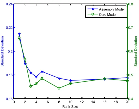
Figure 4.12 Variance Reduction Sensitivity to Rank Estimate...83

Figure 4.13 Standard Deviation Comparison for Thermal Fission Rate Density ...85

Figure 4.14 Standard Deviation Comparison for Thermal Flux ...86

Figure 4.15 Thermal and Fast Scalar Fluxes for Full Core...87

Figure 4.16 Thermal and Fast Scalar Fluxes for Full Core ...88

Figure 4.17 A Cross Section View of the 3-D PWR Quarter Core Model ...94

Figure 4.18 Relative Uncertainty Distribution of Thermal Flux for 1st layer ...95

Figure 4.19 Relative Uncertainty Distribution of Thermal Flux for 2nd layer ...95

Figure 4.20 Relative Uncertainty Distribution of Thermal Flux for 3rd layer ...95

Figure 4.21 Relative Uncertainty Distribution of Thermal Flux for 4th layer ...96

Figure 4.22 Relative Uncertainty Distribution of Thermal Flux for 5th layer ...96

Figure 4.23 Relative Uncertainty Distribution of Thermal Flux for 6th layer ...96

xii

Figure 4.25 Relative Uncertainty Distribution of Thermal Flux for 8th layer ...97

Figure 4.26 Relative Uncertainty Distribution of Thermal Flux for 9th layer ...97

Figure 4.27 Relative Uncertainty Distribution of Thermal Flux for 10th layer...98

Figure 4.28 Histogram of Relative Uncertainty Distribution ...98

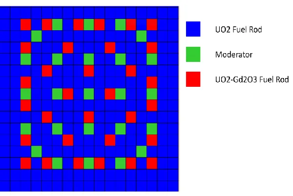
Figure 5.1 PWR Assembly Model ...109

Figure 5.2 Depletion Pattern of the PWR Assembly Model ...113

Figure 5.3 Isotopes of Uranium through the five-cycle-depletion ...114

Figure 5.4 Isotopes of Plutonium through the five-cycle-depletion ...114

Figure 5.5 Speedup of Different Weight Windows through the five-cycle-depletion ...119

Figure 5.6 BWR Assembly Model...120

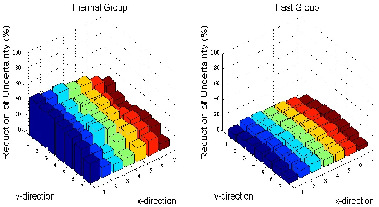
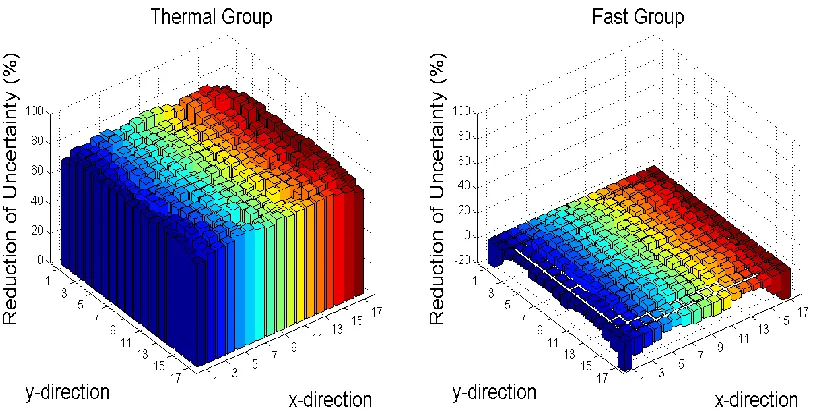
Figure 5.7 Reduced Percentage of Relative Uncertainty in GVR Calculations ...124

Figure 5.8 GVR Calculation Speedup for Fast Group ...124

Figure 5.9 GVR Calculation Speedup for Thermal Group ...125

Figure 5.10 Depletion Pattern of BWR Assembly Model ...128

Figure 5.11 Burnup through Depletion Cycles ...129

xiii

Figure 5.13 FOM Speedup of Capture through Depletion ...134

Figure 5.14 FOM Speedup of Flux through Depletion ...134

Figure 5.15 FOM Speedup of Fission through Depletion ...135

1

CHAPTER 1 INTRODUCTION

The computer simulation of radiation transport within matter is essential to many nuclear engineering applications such as reactor physics design calculations, radiation detection modeling and shielding design. Fundamentally, there are two distinctive methods for modeling radiation transport: the Monte Carlo (MC) and the deterministic (DT) methods. While the two methods are both used to simulate the same type of problems, each method has its unique advantages and limitations.

2

reactor core even with leadership computers. Reactor physicists have therefore resorted to homogenization techniques (described below) to reduce the computational cost. These methods make additional assumptions which are typically refined over many years of experience.

The current commercial reactor design process exclusively utilizes deterministic radiation transport models in conjunction with homogenization techniques to render computationally efficient simulation of the core-wide behavior over the cycles of operation. The reactor design process is typically divided into three stages trading off details in the resolution of energy and space:

1. Infinite medium or 1D transport calculation with high energy resolution (either point-wise of many group representation, e.g. 100s-10000s groups). Cross section resonances are explicitly resolved and appropriately self-shielded. The result of this stage is a self-shielded cross section set comprised of 10s~100s groups.

2. The lattice or assembly level calculation solves the 2D transport equation on a 2D slice of a single assembly using reflective boundary conditions on all four edges which implies the reactor is infinitely loaded with identical assemblies. The flux solution is typically obtained using the Method of Collision Probabilities, the Method of Characteristic or unstructured SN transport solvers.

3

The most attractive feature of MC is its ability to utilize continuous (also referred to as point-wise) energy-dependent cross sections; thereby removing the errors introduced by the multi-group method. In addition to that, MC does not suffer from truncation error present in deterministic models. Moreover, no assumptions about the boundary conditions of each assembly are made. The MC results however are statistical quantities, where the statistical fluctuations are described by a standard deviation. For a reliable MC simulation, the standard deviation on all quantities of interest must be made very small. Due to the central limit theorem, the standard deviation decreases as:

1

, N

  (1)

where is the standard deviation andNis the number of executed histories. For example, a factor of 10 reduction in standard deviation requires a 100 times more particles to simulate, which increases the computational time/cost by the same amount. The standard analog MC simulation is therefore considered impractical without applying powerful variance reduction techniques. Variance reduction techniques minimize statistical errors e.g. by biasing the MC particles towards more important regions in phase space (the basis for importance sampling) or by eliminating the fluctuation in the particles weight.

4

The most widely used variance reduction techniques are Russian Roulette, implicit capture and exponential transformation. For its first couple of decades of application, typical MC problems comprised only a small number of responses such that variance reduction parameters that are instrumental for the above variance reduction methods could be easily devised by hand. However, one typical feature of reactor physics application is that responses are sought everywhere in phase-space and therefore the variance reduction must also be rendered everywhere, e.g., thermal and fast flux everywhere in the core and throughout cycles of depletion; this challenge is known as Global Variance Reduction (GVR).

Recognizing the advantages and deficiencies of both methods, hybrid MC-DT techniques have been proposed by researchers to speed up MC simulation. The essential idea of any hybrid technique is to obtain an inexpensive deterministic estimate of the adjoint or forward flux; then use the estimate to generate variance reduction parameters for GVR. Two typical examples of hybrid MC-DT techniques for GVR are: importance sampling and weight windows. Importance sampling concentrates on the regions in phase space that are most important for the response of interest; weight window controls the particle weight by rouletting and splitting based on the weight function that is derived from the deterministic estimate of the forward or adjoint flux. Common to all hybrid MC-DT methods, a deterministic estimate of the importance function is employed; the difference of hybrid MC-

5

general all hybrid deterministic MC methods address one or several of the following three problems that cause poor MC performance in GVR:

1. Too few particles contribute to the response of interest leading to large relative variance;

2. The magnitude of particle weights that contribute to the response of interest fluctuate;

3. Particles with small weights are retained until collision and cause a waste of execution time.

To overcome the above challenges of current hybrid methods, we present in this work a novel hybrid MC-DT method denoted by the SUBSPACE method. The method is based on the adjoint function and therefore belongs to the same family as the FW-CADIS method developed by the SCALE group at ORNL [33]. For this reason, we employ the FW-CADIS method as a basis for comparison. Similar to FW-CADIS, the SUBSPACE method employs importance maps obtained from deterministic adjoint models to derive automatic weight-window biasing. In contrast to FW-CADIS, the SUBSPACE method does not calculate flux-based weighting of the adjoint source term.

6

7

CHAPTER 2 THEORY

2.1 Deterministic Theory

2.1.1 Forward Deterministic Theory

In the context of reactor analysis applications, the deterministic transport theory is concerned with the solution of the integro-differential form of the forward and adjoint linear Boltzmann transport equation that are originally derived by Ludwig Boltzmann to study the kinetics of gases[50]; it is hereinafter simply referred to as the transport equation. The two forms of the forward transport equation used within this work model the neutron flux in a host medium (1) for the case that the flux is maintained by an external distributed source (fixed source form) and (2) for the case that fission in the host medium maintains the flux without an external source (k-eigenvalue form). In its operator form, the fixed source form of the transport equation is given by the following expression [3]:









L r  E S r  E q r (2) In Eq. (2), the dependent variable 





8

The operatorsLandSare the streaming-plus-collision and the scattering operator given by [3]

respectively:











 



L r E r E

S dE d r E E r E



  

  

    







Instrumental in the definition of these two operators are the macroscopic total and

double-differential scattering cross sections t









sufficient to say here that the macroscopic cross sections are input parameters characterizing the interaction probabilities of the neutrons with the host-medium; we refer to [3] for a comprehensive definition of macroscopic cross sections. The second form of the forward transport equation used within this work is the k-eigenvalue form:

1

,

L S F

k







where the fission operator F is defined as:







 



F dE d r E r E r E

       





Describing the fission process necessitates introducing additional material properties: The

fission cross section _f





9

eigenvalue or multiplication factor k is the ratio of the total neutrons gains in the system and the total neutron losses:

Total neutron gains Total neutron losses

k 

(6)

Depending on the value of the multiplication factor the system is classified as subcritical (k<1), critical (k=1) or supercritical (k>1).

In order to create a well-posed set of equations, boundary conditions have to be specified on the inflow faces:









BC B

r E r E r r

      

(7) where _B is a given function on the boundary and nˆ is the outward normal vector on the domain boundary. Eq. (7) strictly only covers explicit boundary conditions; while in this work we frequently utilize reflective boundary conditions, where the inflow flux depends on the outflow flux in the “reflected” direction. Reflective boundary conditions can be described

by the following equation:



 







ˆ ˆ _ˆ ˆ

, , , ', , and n 0,

ˆ ˆ ˆ ˆ

ˆ ˆ ˆ

n n ', ' n 0

B

r E r E r r

      

10 2.1.2 Adjoint Deterministic Theory

For the derivation of the adjoint transport equation it is necessary to introduce the notion of an inner product over the phase space since the adjoint operators will be defined with respect to this inner product. Let the inner product of the two generic functions f _and g be given

by

0 4

ˆ

, ,

D

f g dE d dV f g







  

where D denotes the spatial domain of the problem. Given a generic operator H _{then its}

adjoint is H†defined by the following relationship:

† † †

,H H , ,

     (10)

where †denotes the adjoint function. The fixed source adjoint transport equation can then be formulated in terms of the adjoint counterparts of the transport-and-collision and scattering operators in a manner very similar to the forward transport equation:

† † † † †

( ),

L S q r (11) where the following definitions are used:









† † ˆ ˆ

, , ,

t

L     r E  r  E (12)



 



† † †

0 4

ˆ ˆ ˆ ˆ

' ' _s , , ', ' , ', ' .

S dE d r E E r E



11

The adjoint source is chosen for the specific purpose that the solution of the adjoint problem has for the user. In general if the user is interested in some system response (e.g. a reaction rate)

, ,

R

R  

(14) then the adjoint source is chosen to the gradient of the response with respect to the angular flux:

†

. R

q 

 

 (15)

In contrast to the forward problem, adjoint boundary conditions need to be given on outflow boundaries:









† ˆ † ˆ _ˆ ˆ

, , _BC , , , _B and n 0.

r E r E r r

       (16)

2.1.3 Discretization of the Transport Equation

Neither the forward nor the adjoint transport equations can be solved analytically for realistic reactor physics applications. Therefore, numerical methods need to be devised such that the transport equation could be discretized in all phase space variables to facilitate its solution on a digital computer. The discretization of the energy variable is performed via the multi-group

formalism; the discretization of the angular space, for the purpose of this work, uses the S_N

12

The multi-group formalism decomposes the range of energy into Gbins numbered from

highest to lowest energy group by g1, ,G such that thegth bin has lower and upper energy boundaries E_g1 and E_g, respectively. Then the transport equation is integrated over

the range of energy bin g and rearranging then gives its multi-group form. Obtaining the

multi-group transport equation is only demonstrated for the forward k-eigenvalue problem since the multi-group forms of the forward and adjoint fixed source equations follow readily from the following development. Consider the multi-group k-eigenvalue equations in operator form:

1

, for 1, , .

g g g g g g

L S F g G

k

      (17)

The group streaming-and-collision, scattering and fission operators, group fluxes and multi-group constants are going to be introduced after the following comments outlining some key features of the derivation of the multi-group transport equations:

1. The angular dependence of the scattering cross section is assumed to be azimuthally isotropic such that its functional dependence can be written in terms of the cosine in between the incoming and outgoing directions. Then the scattering cross sections is expanded into a truncated series of Legendre polynomials:











  

0 2 1 ˆ ˆ , ', ' , , ' , , ' . 4 L

s s sl l

l

l

r E E r E E  r E E P 







       



13

2. The straight-forward way of defining the group total collision cross sections would render it angularly dependent, a feature that is typically not supported by transport solvers. Therefore, some care is taken to define an isotropic group collision cross section.

3. Easier derivations assume energy separability which in practical applications is never satisfied. While the final form of the equations is much simpler its range of applicability is questionable.

Armed with the comments 1 through 3, the definitions pertinent for Eq. (18) of the operators and group angular and scalar fluxes is:

 

 





 



_



_

 

 

 

 

 





 

   

 

0 lg' lg'

0 0 ' 1

' ' ' 1 lg 4 ˆ _,ˆ

! 2 1 ˆ

2

! 4

4

ˆ :Spherical Harmonic of order ,

ˆ ˆ

, , ,

ˆ ˆ _,ˆ

g

g

g g g t g g

L M G

m

g g m lm s g

l m g

G g

g g f _g g

g lm E g E m lm g g

L r r

l m l

S Y r

l m

F r

Y l m

r dE r E

r d Y r

r                                               











 

0g r (Scalar group flux) 

(19)

14



 



 

 



 

_{ }

 



dE r E r E

r

dE r E r E r E

r              



















 



 



 



 

1 ' 1

lg' lg' '

lg lg' lg , ! 4

2 1 !

, , ' , ' , ' g g g g g g g g E g E

s g s g gg tg tlg

E m t l E tlg m E E m sl l E E

s g m

dE r E

l m

l l m

dE r E r E

r

dE dE r E E r E

r                     _    _           









It should be noted that the multi-group equations, aside from the scattering approximation, are exact. However, in the process of the derivation group constants were introduced that depend on the problem’s solution itself such that the equations cannot be solved without

15

The next step in the discretization sequence is to discretize angular variables. Within this work exclusively the SN method is utilized for this purpose. For this method the multi-group

equations are solved only along discrete rays ˆ_n,n1, ,N _{and the scalar flux moments are} then calculated using a quadrature rule that associates a distinct weight w_n for each discrete

ordinate. Integrations over the angular variable are then approximated as follows:

1 4

ˆ N

n n

d w

 

 





(22)

After the discretization of the angular variable we obtained a set of NxG coupled PDEs that continuously depend in the spatial variable. Postponing the treatment of the coupling for later, the spatial variable is discretized by subdividing the spatial domain into non-overlapping cuboidal cells and applying standard methods to discretize the equations on each of these mesh cells. See [49] for various methods; within this work the Step Characteristic method is typically used because it guarantees positive cell average angular fluxes which is important when SN solutions are used in subsequent MC computations.

As the multi-group SN equations are coupled and a direct solution of the global system of

16

The DENOVO code that is used as DT solver uses more advanced techniques, namely it replaces the inner iteration procedure by a GMRES solver which greatly increases efficiency. For a comprehensive description of the solution methods in DENOVO refer to [49].

2.2 Monte Carlo Transport Theory

MC methods are widely applied in computational simulations and especially useful for simulating complicated systems with multiple degrees of freedom. MC methods are a class of stochastic numerical analysis techniques based on the application of random sampling; that is, to evaluate random variables by using random numbers. Random variables are measured through random experiments. In contract to deterministic transport methods that solve an explicit transport equation to obtain the average behavior of particles quantified e.g. by the scalar flux, MC methods infer specific quantities of interest, e.g. the reaction rate in a sub-volume, by explicitly simulating many particles’ life and averaging over the outcome.

Naturally, deterministic methods provide a full set of information for the problem such as fast and thermal fluxes throughout the system, while MC only gives certain information requested by the user, for example, one specific tally in the phase space.

At its core, the MC technique consists of simulating a single particles life from its birth to its destruction. This basic unit of a MC simulation is typically referred to as a history. In general many histories have to be performed to obtain statistically meaningful results.

17

variables. Further, the distance to the next collision site, the collision type and its outcome are random processes as well. From this perspective, simulating a single particle history can be performed using the following basic steps:

1. Through random sampling pick a specific position where a particle is born as well as a specific energy and a specific travel direction;

2. Determine the distance to collision. That is, the distance the particle travels before its first interaction.

3. Determine the type and consequences of the interaction. If the interaction does not lead to an event where the particle is killed; that is, (1) the particle is absorbed or (2) the particle exits the phase space of interest, new energy and direction will be picked through next random sampling and the particle transport will be continued. In particular, if secondary particles are created, for example, if an elastic scattering event takes place, the transport of the secondary particles will be simulated through the same procedure after the primary particle is terminated.

18

At the same time, a new source particle will be selected through random sampling and the same procedure will repeat until the total number of particle histories is successfully simulated.

Fig. 2.1: Incident Neutron Events (referred from MCNP Manual)

Fig. 2.1 illustrates a possible sequence of events for a neutron incident on a slab of fissionable material. The first collision of the neutron within the slab takes place at event 1. The neutron is scattered after the collision in the direction towards 2 while a photon is simultaneously produced and stored for later discussion. At event 2, the incoming neutron is terminated by fission while two emerging neutrons and one photon are born.

The first of the two newly born fission neutrons is captured and terminated in event 3. The other fission neutron leaks out of the slab volume at event 4. The photon produced from the

1. Neutron Scatter, photon

production

2. Fission, photon

production

3. Neutron Capture

4. Neutron Leakage

5. Photon Scatter

6. Photon Leakage

19

fission collides at event 5 and leaks out at event 6. Back to the photon produced at event 1: it is now captured at event 7. So far the simulation history is completed for this incident neutron and the score has been obtained. The MC simulation proceeds by starting another incident neutron and repeats the basic steps that are comprised within a single history.

The transport simulation procedure described above is usually referred as an analog MC simulation. Meanwhile, non-analog MC refers to algorithms where distributions are sampled in a manner to increase the probability that a particle contributes to the quantity of interest and thus reduce the variance of the desired quantity or to control the particle’s weight to ensure that scores do not vary too much in their individual contribution. Hereinafter, certain classes of very difficult problems that require days of computer time with analog MC simulation could be easily solved in hours or even minutes of computer time applying non-analog MC methods.

It is essential for non-analog MC that an unbiased estimate is preserved to ensure the correctness of the simulation. To this end the particle weightw, which indicates the total number of particles that are transported within a single history (think of a “particle package”), is adjusted. In non-analog MC simulations where variance reduction techniques are applied, the weight of the particle is adjusted following the conservation formula below:

0

( ) = ( ) ,

w biased pdf w unbiased pdf

(23) wherew₀ is the particle weight from analog MC simulation before the variance reduction

20

a correct transport simulation so far as the particle weights are conserved during the (biased) transport process.

2.2.1 Probability Theory and Statistical Uncertainties

The statistical uncertainty is a very important quantity in MC transport simulations. As the number of simulated histories is always finite, the estimates of the mean tally values are subject to statistical errors whose magnitude is quantified by the standard deviation. In addition the standard deviations can be used to infer if a tally is statistically well-behaved. If a tally is not statistically well behaved, the true confidence interval will not be reflected corrected by the associated uncertainty and thus the obtained results will be misleading. In

general, for a well behaved tally, the statistical uncertainty will be proportional to 1 2

N , where Nis the number of histories. For well-behaved tallies that means that increasing the number of histories decreases the standard deviation. However, for a poorly behaved tally, the statistical uncertainty may increase as the number of histories increases. By simulating

particle histories, a range of scores{x1, xi, xN}will be generated to each particle history

depending on the selected tally and applied variance reduction techniques. Define f x( )as the probability density function of history score probability, the expected value of scorexis then

defined as true meanx:

( )

x



21

The MC simulation samples the underlying distribution function and obtains a range of

scores{x_1, x_i, x_N}. The range of scores is then used to compute an estimate of the true

mean: x_e, hereinafter referred to as sample mean:

1 1 N e i i x x N 





where x_iis the score ofith particle history sampled from f x( )as stated before, andN is the

total number of particle histories. The sample mean x_eis the average value of {x_1, x_i, x_N}

for all particle histories in the MC problem. The relationship between the true mean xand the

sample mean x_eis described in [4] by the Strong Law of Large Numbers: if xis finite, x_e

tends to the limit of as the historyN methods infinity.

Akin to the true mean, the true variance 2 (i.e: the square of the true standard deviation) can be computed from the underlying distribution function by taking the second central moment:

2 2 2 2

(x x) f x dx( ) x ( ) .x

 

_

variance s2is denoted by:

2 2 1 1 ( ) 1 N i e i

s x x

N 

 

22

The sample variance could also be calculated directly from probability density function f x( ) as shown in the [5] as

2 2 2 2

0

( ) ( ) ( )

x

s x x f x x x









The larger the data set, i.e. the more histories are run in an MC simulation, the more reliable are the sample mean and the sample variance, i.e. the more they are to be close to the true

mean and variance, respectively. In general MC simulations, the sample meanx_e and the

sample variance s2are two representative properties from the probability density function ( )

f x that are of particular interest.

In the above discussion, it is implicitly assumed that the process of interest involves only a single random variable. In reality, processes involve a vector x of random variables which are distributed according to an underlying multi-varied probability distribution function f x( ).

In this case, the variance of the ith random variable is defined analogously to the single variable case:

2 _{( )}2 _{( )} 2 _{( ) .}2

i xi xi f x dx xi xi

 







23

The variance is a special case of the covariance sincecov( ,x x_{i i})_i2 _{. For convenience the} variances and covariances are typically collected in the covariance matrixC:

 





i j

C  x x (31) The covariance matrix is a symmetric positive semi-definite matrix of dimension N [REF], where N is the length of the vectorx. It features the variances on the diagonal and the (true) covariances on the off-diagonals. In section 2.4, it will be shown that the covariances characterize the interdependence of the random variables (i.e. their correlation) such that the properties of the covariance matrix are at a high premium and matrix decomposition can provide valuable information of the system of interest.

The Central Limit Theorem of probability is a very importance theorem for the estimation of the reliability of statistical estimators [4]; it is used to define confidence intervals for the precision of obtained results:

2

/ 2 1

lim Pr[ ]

2

t e

N x _N x x _N e dt

       

     



Where andrefer to arbitrary values andPr stands for the probability. For large N approximation, it could be demonstrated [4] that

2_{/ 2}

1 Pr[ ] 2 t e x x e dt N           



From Central Limit Theorem of probability, it is observed that for largeN approximation the

24

the sample mean x_edistribution is normally distributed with the mean of true meanx. Given

that the sample variances2 is considered equivalent to the true variance 2 for a MC simulation with sufficient particle histories as discussed before, the following two statements on confidence intervals could be deducted from the standard table for the normal distribution:

with 68% confidence 2 2 with 95% confidence

e e

e e

x s x x s

x s x x s

   

    (34)

Within this work, it will be necessary to estimate the statistical uncertainty of derived important quantities that are not directly tallied. However, in general a functional form is known that describes the derived quantities in terms of directly tallied quantities.

Then the law of Error Propagation [5] could be used to estimate the statistical uncertainty associated with the derived quantities:





2

2 2

1

, , , _N : known functional form

N

f i

i i

f x x x

f x        _{ }   







Propagation law is applicable to almost all circumstances in measurements.

It should be noted that the variablesx x₁, ₂, ,x_N are required to be truly independent to avoid

25

As previously discussed, the estimated statistical uncertainty squared 2 should be proportional to1/N . Furthermore, the execution time T of an MC computation is asymptotically proportional to the number of simulated historiesN , because each history

basically follows the same algorithm. Therefore, the product of variance 2

and execution time T is expected to be asymptotically constant for every estimated quantity in MC

simulation. The inverse of the product 2 T

 is defined as Figure of Merit (FOM) of a single tally [6]:

2 1 FOM

T 



(36)

26

The global FOM is thus introduced for comparing different methods to obtain effective variance reduction parameters [7]. As a direct extension of the single-tally FOM, a global FOM is defined for a set of tallies by replacing the single variance by a value representative of the distribution of variances. The single value could be the maximum variance or the mean variance of the tally set. In general, it is desirable to have a small spread of tally variances because the largest variance usually limits the confidence in the simulation’s results. In [7],

four different types of global FOMs are introduced:

2 1 max 1 FOM T 

 (37)

2 1 FOM

vT

 (38)

3

1 ( _v) FOM

v  T



 (39)

4 1/4

1 [ ( _v/ 3) _v] FOM

v   T



 (40)

In above equations, _maxstands for the maximum relative uncertainty in one single tally

throughout the domain; Tstands for the time; v stands for the mean of the variance, _vfor the relative uncertainty of the variance and _vstands for Kurtosis, the peak factor.

weight-27

window maps [7]. In this work, the second form of global FOM is utilized to compare the efficiency of hybrid MC-DT methods in GVR.

2.2.2 Variance Reduction Techniques

The analog MC method mimics the physical process of particle transport: One could say that nature actually plays unbiased MC. However in practice, calculations are expected to produce accurate answers with reasonable efficiency. In MC simulations, variance reduction techniques, also named biasing techniques, are widely employed to decrease the statistical uncertainty  of the desired results while trying to keep the computational time within a reasonable range and more importantly keep the estimates of the mean value unbiased. Two possible solutions to achieve the goal are: 1. Reduce the standard deviation s for a fixed number of histories; 2. Increase the total particle historyN given a fixed amount of time. However, in the most recent history of MC, there has always been a trade-off between these two solutions for the reason that the decrease of susually causes a corresponding increase of

computation time per history; while the increase of total particle historyN would lead to a higher standard deviations [6]. Therefore, variance reduction techniques are applied to

achieve a compromise to decrease swithout increasing the total historyN significantly. Generally, these techniques could be divided into two categories: 1. Techniques that produce particles work by decreasings; 2. Techniques that destroy particles work by increasing the

28

Over the course of last few decades, many variance reduction techniques have been developed. It should be noted though that one technique cannot serve for all application purposes, and different techniques might also contradict with each other if used together. Below is a summary of several of the most widely applied variance reduction techniques:

Source Biasing

In many problems, a large amount of source particles are distributed over space, energy, angle and time. Among them certain particles tend to make more contributions to a specific result compared to other particles and thus are considered of high importance. Source biasing works well for such problems. Source biasing samples from a biased source distribution in phase space; this means the particles of high importance are much more likely to be selected than particles of low importance. The weight of the source particles will be consequently corrected to conserve the total weight of particles in the given interval as well as to preserve an unbiased estimate [6] [8].

Implicit Capture

29 the weight before the collision [9]:

before 1

a after collison collison

t

w w  _  _



  (41) where_a is the absorption cross section and _tstands for the total cross section.

The advantage of implicit capture is that efficiency is increased as particles can be terminated only by transmission or reflection and thus will always be contributing to the calculations without the loss of absorption.

Exponential Transform

Exponential transform, or path stretching, is a technique that biases particles into the desired area by biasing the distance between collisions. When a particle is moving towards the detector, distances that are greater than one mean free path would be sampled. When a particle is moving away from the detector, distances that are shorter than one mean free path would be sampled. After the sampling, the total macroscopic cross section would be modified as [9]:

mod

(1 )

ified original

t t p

    (42)

wherep is an exponential transform parameter to vary the degree of biasing, and is the cosine of the angle between sampled direction and the original direction.

30

technique is particularly useful for deep-penetration transport problems where a source particle has a slight chance to method the detector.

Splitting with Russian Roulette

Splitting in MC simulation usually contains three categories: geometry splitting, energy splitting and time splitting [6] [9].

Geometry splitting is a variance reduction technique extensively employed in Monte Carlo codes. The essential idea of geometry splitting is to increase the number of particles moving towards a desired direction of interest while particles moving towards an uninterested direction are killed to avoid wasting further efforts. Geometry splitting divides the problem geometry into a set of cells and each cell is assigned with an importanceI. If a particle of a

weightwmigrates from a cell of importanceI_{k to a cell with a higher importance}I_j, the

particle will be split into a number ofnI_j/I_k identical particles each of the weightw n/ .

On the other hand, if a particle of a weightwmigrates from a cell of importanceIkto a cell

with a lower importanceI_j, Russian roulette will be played, and the particle will be killed

31

Energy splitting works similarly to geometry splitting. It is performed on the energy space and independent of spatial cell. Particles could be split when they pass in between different energy ranges and Russian roulette is played correspondingly to reduce the particle number and computational time.

Time splitting is similar to the above two types of splitting, except a particle’s time could only increase. Since particles are more important later in time for certain circumstances, it is more useful to split particles as time increases. One example is the case where a detector responds primarily to late time particles. If too many late time particles exist, the late time particles could be roulette to preserve reasonable calculation efficiency [6].

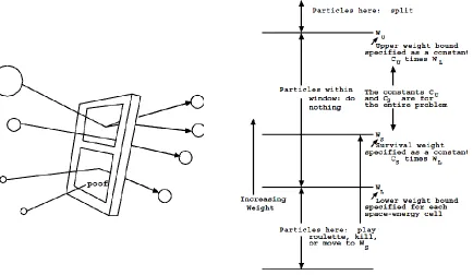
Weight Window

The weight window [6] is a representation of phase space splitting and Russian roulette technique implemented in the MCNP code. The phase space could stand for space, space-energy or space-time. Figure 2.2 below borrowed from MCNP manual provide a detailed presentation about how the weight window technique works.

32

There are several importance differences between weight window technique and geometry split/roulette technique although they work in the similar way [6].

Fig. 2.2: Weight Window (referred from MCNP manual)

L

W , the lower weight bound.

S

W , the survival weight for particles playing roulette

U

W , the upper weight bound.

1. Geometry splitting is only space dependent while the weight window is space-energy dependent or space-time dependent.

33

3. The weight window could be applied at surfaces or collision sites or both. Meanwhile, splitting could be only employed at surfaces.

4. The weight window is able to control fluctuations of particle weight introduced by other variance reduction techniques while the geometry splitting is weight independent and preserve weight fluctuations.

5. The weight window could be turned off for selected energy or space regimes.

The weight window could be generated by the weight window generator. A weight window generator generates weight window importance functions automatically [6]. Dividing the phase space into a number of different phase space “cells” or regions, the importance of a cell is then defined as the expected score generated by a unit weight particle after entering the cell. Therefore, the cell’s importance is estimated as:

score due to the particles entering the cell Importance

weight entering the cell total

total 

(43)

34

2.2.3 Variance Reduction based on the Adjoint Function

In MC particle transport problems, to calculate the response at a certain location is equivalent to computing the following integral:

( , ) ( , )

d

d V E

R

 

Using the fundamental property of the adjoint equation †,H  H† †, ,

the response R_{at a certain location could also be introduced as:}

( , ) ( , )

S V E

R

 

(45) where is the adjoint flux, q is the source density over the source volume V_S.

The adjoint function represents the particle importance with respect to the corresponding response. However, the evaluation of Eq. (45) requires knowledge of the adjoint function that is typically not available in a closed form. Instead, an approximation of the adjoint flux is employed to generate an importance map and a biased source [8]. Based on the adjoint

function, Wagner introduces an alternative pdf q r Eˆ( , ) to replace the original pdf q r E( , )[8]:

( , ) ( , ) ˆ( , ) , ˆ( , )

S

V E

r E q r E

R q r E dEdV

q r E 

35 where q r Eˆ( , ) is given by:

( , ) ( , ) ˆ( , )

( , ) ( , )

S

V E

r E q r E q r E

r E q r E dEdV 



 



 

This is a typical example of importance sampling. However, since the adjoint function is not exact, MC simulations for particle transport are necessary. As stated before, in source biasing, the weight of a source particle is corrected as

0

( , ) ( , ) ( , )

w r E q r E w q r E (48) where w₀is the unbiased weight of a particle and usually set equal to 1. By substituting the

equation (47) into equation (48), the following result could be obtained:

( , ) ( , ) ( , )

( , ) ( , )

S

V E r E q r E dEdV R

w r E

r E r E



 



 



 

which shows an inverse relationship between the adjoint function and the particle weight. In this way, the target weight matches the particle’s energy and position precisely. This

relationship has been verified through computational analysis in [14] as well as been derived in [8].

In [8], it is demonstrated that the number of particles emerging in( , )r E from an event in ' '

( ,r E)is adjusted by the ratio of importance:

' ' ( , ) ( , ) r E r r E    

36

Ifrgreater than 1, particles are created by splitting; if rlower than 1, particles are destroyed through rouletting. Employing the ratior, the following equation could be obtained as shown in [8]:

' '

' ' ( , ) ( , ) ( , )

( , ) r E

w r E w r E

r E  

 

 (51)

Since the above relationships for the particle weights were derived from importance sampling in a consistent manner, it is referred to as the CADIS (Consistent Adjoint Driven Importance Sampling) method [8] and is implemented in SCALE 6.1 code sequence [24]. The CADIS method uses a discrete ordinates code to determine the adjoint particle flux. The obtained adjoint flux, regarded as the importance of particles, is employed in generating the biased source and corresponding weight window map [1]. The adjoint-flux-based importance map is required to be consistent with the source biasing to avoid insufficient survival particles that will cause a waste of computational time.

An extension of the CADIS method, forward-weighted CADIS (FW-CADIS) is considered a state-of-art variance technique [10]. It is developed by applying an inexpensive discrete ordinates code to perform a forward Sn calculation to estimate the expected tally responses. The adjoint sources that correspond to each tally are weighted inversely by the forward tally estimate. Then the standard CADIS is applied with an importance map and a biased source that are generated using the adjoint flux computed from the adjoint Sn calculation.

For example, in order to calculate a detector response function _d( , ) r E over a mesh tally,

37

( , )

( , ) ,

( , ) ( , ) dE

d d

r E q r E

r E r E



 

 _



where ( , ) r E is an estimate of the forward flux.

In the current implementation in SCALE 6.1, two options for forward weighting are available [24]:

1. For tallies where the entire group-wise flux is required with low relative uncertainties, the

adjoint source should be weighted inversely by the forward flux( , ) r E ;

2. For tallies where only an energy-integrated quantity



The table below from SCALE 6.1 MAVRIC Manual shows how the adjoint source is

weighted by certain quantity to optimize the forward Monte Carlo simulation at multiple tally locations [24]:

Table 2.1: Adjoint Source Weighting in FW-CADIS

Calculation Adjoint Source

Energy and spatial dependent flux ( , ) r E ( , ) 1 ( , ) q r E

r E 

 _

Spatial dependent total flux



r E dE 

 _



Spatial dependent total dose rate



( , ) ( , )

d d

r E q r E

r E r E dE



 

 _

38

The overall goal of FW-CADIS is to achieve the particle density uniform over MC tallies via an importance map based on adjoint flux information. By obtaining more uniform particle densities, more uniform relative errors for the tallies will be realized. FW-CADIS has been proven to be a powerful GVR technique in many applications [10].

2.2.4 Correlation of Responses in MC Simulation

A correlation in statistics refers to inter-dependence of two (or in general more) random variables, i.e. how does one variable change if another one is changed or in the extreme of total correlation: does fixing one random variable totally determine another random variable. For example, the median income of a school district can be conjectured to be correlated to the average SAT scores within this district, because, in general, the richer the area the better the school. Correlations often (not always) imply an underlying causality but do not investigate or require it between the two correlated quantities. For example fact Z can cause both X and Y such that X and Y are correlated. However, X and Y can be completely unrelated in terms of a causal relationship.

39

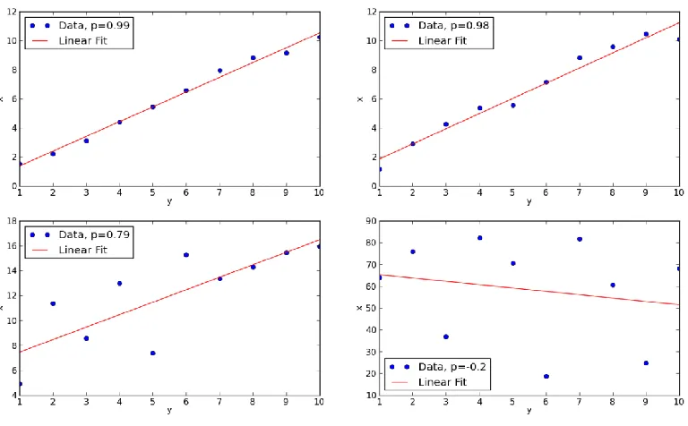
The most commonly used correlation coefficient was introduced by Pearson and is defined as [40]:

,

cov( ,_{i j})

i j

i j

x x p

  

(53)

where cov( ,x x_{i j}) stands for the covariance between variablesx_iand x_j; _iand _jstands for the relative uncertainty of each variable.

An important property of Pearson’s correlation coefficient is that it is only sensitive to linear

correlations: A linearly uncorrelated, but non-linearly highly correlated phenomenon would seem to be uncorrelated when only Pearson’s correlation coefficient is used. Values of the

correlation coefficient range from -1 representing a perfectly negative linear correlation to +1 representing a perfectly positive correlation. In any of these limiting cases a random variable is totally determined by fixing another random variable by a relationship of the form:

.

i j

x  mx c (54) Totally uncorrelated variables exhibit a correlation coefficient of zero, but the converse, i.e. a zero correlation coefficient implies uncorrelated random variables, is not true because random variables can be correlated non-linearly. It is, however, true that a zero correlation coefficient implies that random variables are linearly uncorrelated.

40

lowest correlation of a negative correlation coefficient -0.2. The most correlated data set 0.99

p has the best linear fit while the least correlated data set p 0.2 has the worst linear fit.

Fig. 2.3: Pearson’s Correlation Coefficients

41

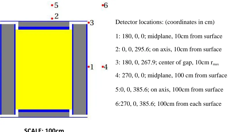
A full-size cylindrical cask model from SCALE 6.1 manual [24] is employed to show such correlations between responses. Neutron flux responses are detected at 6 different detector locations as shown in the Fig. 2.4. Detector 1 and 4, Detector 2 and 5, Detector 3 and 6 are located very close to each other respectively. The adjoint flux profile for each detector is plotted separately in the Fig. 2.5. It is quite obvious that the detector 1 has the most similar adjoint flux profile to detector 4. The same similarity also exists in between detector 2 and 5, detector 3 and 6.

42

SCALE: 100cm

Fig. 2.4: Cask Geometry and Detector Locations from SCALE 6.1 Manual

Fig. 2.5: Adjoint Flux Profiles of Detector 1~6

Detector locations: (coordinates in cm)

1: 180, 0, 0; midplane, 10cm from surface

2: 0, 0, 295.6; on axis, 10cm from surface

3: 180, 0, 267.9; center of gap, 10cm rmax

4: 270, 0, 0; midplane, 100 cm from surface

5:0, 0, 385.6; on axis, 100cm from surface

43 2.3 Monte-Carlo-Deterministic Hybrid Method

Over the course of the last five decades, there has been a growing interest in coupling Monte Carlo and deterministic methods employing a hybrid method to combine their benefits and overcome some of their individual deficiencies [1],[2],[16],[19],[21],[33]. The main idea is to bias Monte Carlo sampling using an estimate of the solution obtained inexpensively from a simplified deterministic model. In the Monte Carlo community, this procedure represents a form of “Variance Reduction”. Among the variance reduction techniques, splitting/roulette and implicit capture have been the most widely applied techniques for reducing the variance of the Monte Carlo calculations [17]. These techniques, together with many others, are available in most standard Monte Carlo codes including MCNP [6], TRIPOLI [22], MORSE [26], and MCBEND [42].

These techniques have been successfully demonstrated to reduce the variance for a single response [1], [13], [16] often representing a functional of the solution over a region in the phase space, i.e., a detector’s response in a given region. Examples are the TRIPOLI MC

44

Lift Method employs an approximation of the exact adjoint solution to approximate the zero-variance method for the source-detector problem, and therefore overcomes the difficulty of searching the exact solution of the adjoint transport problem. This approximation uses a deterministic adjoint calculation to obtain localized biasing parameters for source biasing, collision biasing and path length biasing [43].

When these methods prove to be powerful, nevertheless, they are very sensitive to the accuracy of the importance function, require additional user input and are statistically instable compared to the splitting/roulette methods alone [31]. Furthermore, once the problem is expanded from a detector to a large region, Global Variance Reduction (GVR) becomes the primary goal, especially when Monte Carlo methods are to be used for reactor analysis applications. In this case, the above methods are no longer effective for the purpose.

As stated before, GVR denotes problems where one seeks to reduce the variances for all responses evaluated everywhere in the phase space, such as group fluxes, reaction rates density, and homogenized few-group cross-sections. Therefore a uniform distribution of MC particles throughout the domain is crucial. Responding to this challenge, a number of methods have been developed in the field. In general, these methods could be divided into two categories: i) Methods that employ a deterministic forward flux solution as the basis of a