Radiation Source Mapping with Bayesian Inverse Methods.

A B S T R A C T

HYKES, JOSHUA MICHAEL. Radiation Source Mapping with Bayesian Inverse Methods. (Under the direction of Yousry Y. Azmy.)

We present a method to map the spectral and spatial distributions of radioactive sources using a small number of detectors. Locating and identifying radioactive materials is important for border monitoring, accounting for special nuclear material in processing facilities, and in clean-up operations. Most methods to analyze these problems make restrictive assumptions about the distribution of the source. In contrast, the source-mapping method presented here allows an arbitrary three-dimensional distribution in space and a flexible group and gamma peak distribution in energy. To apply the method, the system’s geometry and materials must be known. A probabilistic Bayesian approach is used to solve the resulting inverse problem (i p) since the system of equations is ill-posed. The probabilistic approach also provides estimates of the confidence in the final source map prediction. A set of adjoint flux, discrete ordinates solutions, obtained in this work by the Denovo code, are required to efficiently compute detector responses from a candidate source distribution. These adjoint fluxes are then used to form the linear model to map the state space to the response space. The test for the method is simultaneously locating a set of 137

Cs and 60

© Copyright2012by Joshua Michael Hykes Some Rights Reserved

This work is licensed under a

Creative Commons Attribution-NonCommercial-NoDerivs 3.0United States License.

To view a copy of this license, visit

http://creativecommons.org/licenses/by-nc-nd/3.0/us/

or send a letter to Creative Commons 444 Castro Street, Suite900

Radiation Source Mapping with Bayesian Inverse Methods

by

Joshua Michael Hykes

A dissertation submitted to the Graduate Faculty of North Carolina State University

in partial fulfillment of the requirements for the degree of

Doctor of Philosophy

Nuclear Engineering

Raleigh, North Carolina 2012

APPROVED BY:

Dmitry Y. Anistratov John Mattingly

C.T. Kelly Yousry Y. Azmy

B I O G R A P H Y

A C K N O W L E D G E M E N T S

Primary credit goes to my advisor, Dr. Yousry Azmy, who is both an effective and caring guide. Dr. Anistratov offered several practical suggestions in this work and pointed me toward related work in other fields. Dr. Cacuci introduced me to many of the concepts relating to sensitivity and uncertainty analysis. Dr. Mattingly’s expertise in radioactive sources and detector systems was especially valuable, without which I would still be conducting the experiment described in this thesis. Dr. Kelly’s class on optimization turned out to be more useful than I expected for this project.

Gerald Wicks assisted me in finding a laboratory room and radioactive sources. I appreciate the help of Dr. Gardner and his graduate students (Jiaxin Wang, Zhijian Wang, Wesley Holmes, and Adan Calderon). They are experts in understanding and obtaining detector response functions for the2×2sodium iodide detector.

I also appreciate the encouragement from and camaraderie with my fellow Nuclear Computational Science Group members: Dan Gill, Joe Zerr, Sebastian Schunert, Sean O’Brien, Sameer Vhora, and Brian Powell. Without them, my time in graduate school may have been slightly shorter than it was, but it would have certainly been drearier.

Finally, I must recognize the support of my family. In more ways than one, I would not be here without my parents. My wife demonstrated hope, patience, and encouragement as the last stages of the research and writing seemed to never end.

TA B L E O F C O N T E N T S

LIST OF TABLES . . . vi

LIST OF FIGURES . . . viii

Chapter 1 Introduction . . . 1

Chapter 2 Solving inverse problems . . . 8

Chapter 3 Inverse radiation transport review . . . 33

Chapter 4 Source mapping methods . . . 49

Chapter 5 Source mapping in a controlled environment . . . 73

Chapter 6 Conclusions and future work . . . 109

Appendices . . . 123

Appendix A Responses and the adjoint flux . . . 124

Appendix B Gamma cross section uncertainties . . . 134

Appendix C Source mapping experiment . . . 136

Appendix D Detector efficiencies . . . 160

Appendix E Radiation source reconstruction with known geometry and materials using the adjoint . . . 168

L I S T O F TA B L E S

Table 4.1 Parameters for source inversion. . . 59 Table 5.1 The energiesEand group indexifor the16energy group structure

used for this test problem. The structure is based on the fine-group gamma shielding cross section library from s c a l e.11 Energies, in keV, are the upper limit of the respective group. The groups above 60

Co’s highest peak (1.332 MeV) and below 100 keV are omitted. . 78 Table 5.2 Comparing the predicted source emissions against the true

inten-sities. The intensities are in total emissions per gamma line per second. They are summed over all spatial cells. The true source intensities are computed with the activities from Tablec.4and the yields from Table c.2. Unless noted otherwise, the initial guess was set to ten,~αinit =10. . . 88 Table 5.3 Comparing the predicted source emissions per energy per second

summed over space against the true values for the carpet test problem. . . 108 Table a.1 Description of the problem for numerical-adjoint test. The spatial

domain is a 5 cm cube, with x,y,z ∈ [0, 5]. Vacuum boundary conditions are applied, thus eliminating the need for the bilinear concomitant. . . 126 Table a.2 Comparison of relative inner product difference_e of Equationa.4

for various t o r t and Denovo spatial discretizations and flux convergence criteria. . . 127 Table a.3 Numerically-adjoint spatial discretizations in t o r t and Denovo

in the test. . . 128 Table b.1 Estimated uncertainties in photoelectric cross section in e p d l 9 7

(assumed to be1_σ). . . 135 Table c.1 Detector components used in experiment. All components are

branded Ortec except the NaI crystal. . . 140 Table c.2 137Cs and 60Co radioisotope properties. Gamma energies and

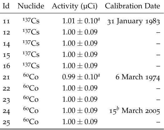
branching fractions are from n n d c.15 Half-lives are from n i s t.116141 Table c.3 The137Cs and60Co sources used in this experiment, with their

Table c.4 Estimated sources activities based on computed activities of dated sources11,21, and 24and on the measured peak area ratios. For each undated137

Cs source, there is one peak and one dated137 Cs reference source, so we have only one activity estimate. For each undated60

Co source, there are two dated60

Co reference sources and two peaks, yielding four activity estimates. The reported activity (and the derived 1 µCi date) are based on a weighted average of the four estimates. . . 145 Table c.5 The elemental composition of materials used in the2144 model.

The densities and compositions are from the Standard Composi-tion manual of s c a l e.11 Integer values of composition are the atomic abundance per molecule, while real values indicate atomic weight percent. . . 148 Table c.6 Source locations for60Co. All dimensions are in cm. Theylocation

of all sources was 9.5 cm, and 90.2 cm forz. All the137

Cs sources (IDs 11-16) were located at (440, 5, 1) cm. . . 152 Table c.7 Detector locations. All dimensions are in cm. . . 152 Table c.8 Gamma particle energies present in background. These were used

in energy calibration. The peak energies are from the National Nuclear Data Center.15

. . . 156 Table c.9 The normalized _χ2-value for the four peak fits in Figure c.10.

The expected normal distribution around one for the normalized

χ2/ndof is also provided. All of the fits except for the 40K peak fit

fall less than two standard deviations from the mean. . . 159 Table d.1 Peak and total intrinsic efficiencies for the bare and collimated

de-tectors, as well as the mean chord length, as computed by m c n p. The one-sigma uncertainties are derived from the Monte Carlo statistical errors. For reference, the mean chord length predicted by the Dirac formula is3.387cm. . . 165 Table e.1 Description of the source-reconstruction problem. All faces had

vacuum boundary conditions. . . 173 Table e.2 Comparison of number of transport solves needed for the adjoint

L I S T O F F I G U R E S

Figure2.1 Direct problem. . . 9 Figure2.2 Inverse problem—causation. . . 10 Figure2.3 Inverse problem—model identification. . . 10 Figure5.1 The true distribution of the 137Cs and 60Co sources, as

repre-sented on the Cartesian computational mesh. The137

Cs sources are grouped together in a point source, and the60

Co sources are aligned in a row parallel to thex-axis. The natural logarithm of the source intensity is plotted, that is, log_e(qpijk/q0), where q0

is a unit scalar needed to make the argument of the logarithm dimensionless and qpijk is the source in peak p in spatial cell (i,j,k). The units ofqpijk andq0are particles emitted per second.

In reality, the blue cells have no sources, but they are shown here with small source intensities to aid comparison with the results presented below. . . 75 Figure5.2 A comparison of the measured and computed responses for the

source mapping with photopeak synthetic responses. . . 84 Figure5.3 Volume rendering of the mean of the posterior distribution of

the source using the photopeak synthetic responses. The source prediction has suppressed source regions in cells around the primary source cells. This results in dark areas near the sources visible in the insets. . . 85 Figure5.4 Slices in the x-y plane of the mean (upper plot) and standard

deviation (lower plot) of the posterior distribution of the source using the photopeak synthetic responses. The natural logarithm of the source intensity is plotted, that is, log_e(qpijk/q0), where q0

is a unit scalar needed to make the argument of the logarithm dimensionless. The units ofqpijk andq0are particles emitted per

second. . . 86 Figure5.4 Slices in the x-y plane of the mean (upper plot) and standard

deviation (lower plot) of the posterior distribution of the source using the photopeak synthetic responses. (continued) . . . 87 Figure5.5 Change in chi-square and the number of function evaluations

with respect to the intensity of the uniform initial guess for optimization. . . 89 Figure5.6 The local minimum reached when using~_αinit = −6. The slices

Figure5.7 Slices in the x-y plane of the mean (upper plot) and standard deviation (lower plot) of the posterior distribution of the source using the photopeak synthetic responses with a favorable initial guess,~αinit =1. . . 91 Figure5.8 Change in source intensity summed over space with respect to

the initial guess for optimization. The upper, cyan horizontal line corresponds to the true value of the662keV peak, while the lower, blue line corresponds to the intensity of the two60

Co peaks. The shaded area around a line represents the1_σconfidence interval about the mean. . . 92 Figure5.9 Measured and computed responses for the source mapping with

synthetic photopeak and continuum responses. For indices where no “computed with true source” data point is present, the value is off the bottom of the scale. See Figure5.2for an explanation of the absolute and relative error plots. . . 94 Figure5.10 Slices in the x-y plane of the mean (upper plot) and standard

deviation (lower plot) of the posterior distribution of the source using both the photopeak and continuum synthetic responses. The natural logarithm of the source intensity is plotted, that is, log_e(qpijk/q0), where q0 is a unit scalar needed to make the

argument of the logarithm dimensionless. The units ofqpijk and

q0 are particles emitted per second. . . 95 Figure5.10 Slices in the x-y plane of the mean (upper plot) and standard

deviation (lower plot) of the posterior distribution of the source using both the photopeak and continuum synthetic responses. (continued) . . . 96 Figure5.10 Slices in the x-y plane of the mean (upper plot) and standard

deviation (lower plot) of the posterior distribution of the source using both the photopeak and continuum synthetic responses. (continued) . . . 97 Figure5.11 Measured and modeled scalar flux for the experiment in 2144

Figure5.12 Measured and computed responses for the source mapping with experimental data. For indices in the top subplot where a data point is missing, the value is off the bottom of the scale. See Figure5.2 for an explanation of the absolute and relative error plots. The Denovo-computed response using the true source distribution for the662keV peak at location2looking in the+z direction is about100 times too large. This is because the137Cs source is located within the fuzzy region around cosθ =µ =0

modeled in Denovo (see section 4.5.3). This inaccuracy is also present in Figure5.2and Figure5.9a, but it is obscured there by the larger number of responses. . . 101 Figure5.13 Slices in thex-yplane of the mean (upper plot) and standard

devi-ation (lower plot) of the posterior distribution of the source using the photopeak responses of the experimental data. The natural logarithm of the source intensity is plotted, that is, log_e(qpijk/q0),

where q0 is a unit scalar needed to make the argument of the

logarithm dimensionless. The units ofqpijk andq0are particles

emitted per second. . . 102 Figure5.14 The true distribution of the137Cs and60Co sources for the carpet

source problem. In reality, the blue cells have no sources, but they are shown here with small source intensities to aid comparison with the results presented below. . . 104 Figure5.15 Measured and computed responses for the source mapping with

the carpet source. For indices where no “computed with true source” data point is present, the value is off the bottom of the scale. See Figure5.2 for an explanation of the absolute and relative error plots. . . 105 Figure5.16 Slices in the x-y plane of the mean (upper plot) and standard

deviation (lower plot) of the posterior distribution of the source using the photopeak responses for the floor-distributed source. The natural logarithm of the source intensity is plotted, that is, log_e(qpijk/q0), where q0 is a unit scalar needed to make the

argument of the logarithm dimensionless. The units ofqpijk and

q0 are particles emitted per second. . . 106 Figure5.16 Slices in the x-y plane of the mean (upper plot) and standard

deviation (lower plot) of the posterior distribution of the source using the photopeak responses for the floor-distributed source. (continued) . . . 107 Figurea.1 Demonstrating the non-uniform mesh for the test problem. This

Figurec.1 A schematic of the detector components. . . 140 Figurec.2 The six137Cs sources and five60Co disc sources. Each source is

labeled with the source id used throughout this experiment. . . . 143 Figurec.3 Slices from thex-yplane of the 2144 b e l room layout. . . 146 Figurec.4 Pictures of the2144room. . . 147 Figurec.5 The count times for two counting sets. Each histogram bin is one

hour wide. . . 149 Figurec.6 The source and detector configuration for the source-strength

counts. . . 150 Figurec.7 The137Cs and60Co source locations. . . 151 Figurec.8 The2_πcollimated detector. The lead bricks are 2×4×8 inches in

dimension. The blocks with a hollowed cylinder have an outside side-length of4inches and a height of2inches. . . 153 Figurec.9 The IDs of the detector measurements that were taken. . . 154 Figurec.10 A representative background spectrum taken with the NaI detector.159 Figured.1 Lead collimation around NaI detector crystal. . . 164 Figured.2 Measured and modeled photopeak responses. No137Cs and60Co

measurements were taken from location5. The experiment value is zero where there is no blue experiment point accompanying a green model (predicted) value. . . 167 Figuree.1 Reconstructed source using81detector locations. . . 173 Figuree.2 Reconstructed sources using adaptive procedure and “aligned”

detectors. Each filled circle or x-mark denotes one source un-known. The detectors are located at the source unknowns. . . 176 Figuree.3 Reconstructed sources using adaptive procedure with

evenly-spaced detectors. The plus marks indicate thex position of the detectors. The vertical positioning of the pluses on the graph is meaningless. . . 177 Figuree.4 Reconstructed sources using adaptive procedure with Monte

Carlo forward flux. . . 178 Figuree.4 Reconstructed sources using adaptive procedure with Monte

Carlo forward flux. (continued) . . . 179 Figuref.1 Two-dimensional representation of a mapping T. Here Tx₁=y₁

1

Before describing our new approach towards resolving the radiation source mapping problem, we first give a full description of the problem which we intend to solve. This is the goal of this chapter, as well as discussing potential applications of the developed methods. Also included is an outline of the remainder of this thesis.

1.1 d e f i n i n g t h e p r o b l e m

The goal of this work is to build a map of the distribution of radioactive sources in a structure using limited detector measurements. Because there could be a number of variations on this problem, depending largely on what information is assumed known or unknown, we spend the following sections giving an account of the approach we have chosen. These details are delineated according to the known information, the unknown information, assumptions which we accept in order to solve the problem, and the external data and tools available.

1.1.1 Knowns

of this work, engineers are exerting significant effort in methods to automatically build maps of an unknown building.1,105

This is often necessary for autonomous robots. Thus, the lack of prior knowledge of a structure may not eliminate the applicability of the methods here described, as long as an automated geometry mapping tool is available.

Closely related to the geometric configuration, the elemental composition and density of each material in the space is needed so that the macroscopic cross sections can be computed. However, precise data may not be required or necessary; this data could be estimated for most standard materials (such as concrete block walls or steel pipes).

The other information we require is radiation detector measurements. Here we focus on gamma (photon) detection, mainly for the ability to measure the energy spectrum of the gammas. In addition, high-energy photons are able to pass through thick materials, potentially increasing the information which our detector collects. Although neutrons are also highly penetrating, we lack the ability to measure the energy distribution of neutrons and so must typically settle for gross-counts, summing over all energies.

The multichannel analyzer (m c a) records the energy deposited by photons in the detector. This distribution comprises both photopeaks and the smooth continuum. The photopeaks are produced by uncollided photons (that is, photons which were emitted from the source and have made their first interaction within the detector) that deposit all their energy in the detector. The continuum portion of the spectrum is caused by scattered photons and by photons which deposit only a fraction of their energy in the detector. Analyzing the photopeaks is much simpler than analyzing the full spectrum. In this work, we desire the flexibility to analyze the photopeaks alone, or the continuum along with the photopeaks. Thus, capturing the effects of scattered photons is necessary.

1.1.2 Unknowns

We are primarily interested in the distribution of radioactive sources, in both energy and space. The location and energy spectra of the sources are initially unknown to us. The goal is to estimate the source map q(~r,E) over the domain of interest. We are not attempting to find the location and strength of a point source or of several point sources. Although the point source model is often sufficient, in this work we desire the ability to estimate distributed sources. Imagine, for instance, estimating the source density in contaminated water covering the floor of a basement room of a nuclear power plant after an accident. For measurements taken near the water, a point source approximation will be considerably lacking. As this example illustrates, one may not know exactly where a source is located, but it may be obvious that certain areas can be ruled out, for instance, the air above the contaminated water. Our method should allow one to exclude these regions without diminishing the generality of the new approach.

In this work, more emphasis is placed on the spatial dependence of the distribu-tion. However, that is not to say that the energy dependence is ignored. Algorithms to reconstruct the sources’ energy spectrum, usually with the goal of predicting the radionuclides present, have received much study over the past few decades.34 Identifying radionuclides is outside the scope of this project.

While we are narrowing the scope of this project, we should note two further choices that limit the reach of the developed approach. First, we study situations in which the radioactive source does not change the material properties of the system, most importantly the macroscopic cross sections. This means that the problem of estimating the activity of a significant mass of a chunk of highly-enriched uranium is outside the scope of this project, since the uranium will self-attenuate and scatter some of the emitted gamma rays. On the other hand, these methods would be applicable to situations where low concentrations of a radionuclide are dissolved in water, or for a thin dusting of a source on the surface of walls, floor, or ground.

1.1.3 Available data and tools

Attempting to solve this problem is only possible through the use of a wealth of prior data and tools to predict the detector response given a particular physical system. These tools and data are briefly described below.

Microscopic cross section libraries To predict the interaction of gamma rays with

mat-ter, and the flux of gammas throughout the system, macroscopic cross sections are required. These macroscopic cross sections are computed from the atomic number density of the nuclides constituting a material and these nuclides’ microscopic cross section. Thankfully, the microscopic data for gamma rays is tabulated by e n d f16 and e p d l 9 720 for all materials and energies of interest here. As described in Ap-pendixb, one area in which the e p d l 9 7 lacks is an explicit, quantitative estimate of the uncertainty of these gamma cross sections.

Neutral-particle radiation transport codes Radiation transport simulation codes require

as input (at a minimum) a description of the geometry, material cross sections, and radioactive source description, and they produce an estimate of the particle flux throughout the spatial and energy domain. These codes, executed in adjoint mode, are also able to compute the sensitivity of measurements to various parameters. The level of sophistication, efficiency, and fidelity of these codes is what allows one to undertake an inverse problem such as we have outlined here. Throughout this work, both deterministic and Monte Carlo codes are used, primarily Denovo27

and m c n p.80

Detector energy calibration While this should be part of a basic detection experiment,

we mention here the importance of knowing the mapping between m c a bin number and deposited energy. This is typically performed using a calibration source with multiple peaks of known energy.

Detector response function The detector response function (d r f) provides a mapping

1.1.4 Computational resources and constraints

As the goal of this project is to develop a proof-of-principle of the proposed approach, meeting stringent operational constraints is not of primary concern at this stage. While some inverse transport problems require that the calculation complete in a second or two,77

we are under no such constraints here. In addition, we take the liberty to use high-performance computing resources, where applicable, that are typically unavailable in the field. Obviously these are important issues that must be resolved in future work if the developed method is to find acceptance among practitioners charged with locating and identifying radiation sources.

1.2 p o t e n t i a l a p p l i c a t i o n s

The prototypical application for the methods developed here is a room with a number of radioisotope source distributions – emitting neutrons, gamma rays, or both. We have physical access to the room to make detector measurements and to make note of the geometric shape and material composition of the room, whether in its original condition or having been modified by malicious acts or via an accident. Normally this could be done directly by a technician, but a robot could also perform the task remotely if exposure to the radiation field poses health risks. After obtaining the detector readings and the information about the geometry and materials configuration, an analyst would feed these as input to the proposed methods. The final result would be an estimate of the locations, activities, and energy spectra of the sources in the room and an estimate of the confidence level of the results.

One could imagine a number of related applications, some of which would require modifications or extensions to the methods here proposed.

• Estimating a radiation source map for a building could be useful in a number of situations. Of course, it would be useful for rescue or cleanup following the dispersal of nuclear materials throughout the building. In addition, preemptive scanning of a building or public area could help decision makers in the event of a radiological emergency to better judge between abnormal and normal radiation source levels.

• Inspectors of nuclear facilities currently get estimates of the quantity of nuclear materials caught in pipes using specialized instruments.95

these “hold up” measurements might be improved with a better estimate of where the source material is lodged.

• Detectors carried by airplanes or helicopters are used to map the radiation source on the ground, for instance, in the aftermath of the Fukushima Daiichi accident. To see the results of one such survey, see the n n s a dose maps on page 17 of Ref. [62].

• Instead of using radiation portal monitors at border crossings to detect sources in only their own lane of traffic, an array of detectors feeding an inversion algorithm could give more detailed information about sources in several lanes. • On a larger scale, the radiation field in a facility could be retroactively

recon-structed using the readings of the detectors worn by their workers.

• This method could potentially be extended to detect a missing fuel rod in an assembly.

This is not an exhaustive list of potential end applications. The methods that we develop in this work are general enough to be applied in a variety of other settings.

1.3 o u t l i n e o f t h i s d o c u m e n t

The rest of this thesis is structured as follows.

• Chapter 2is a broad introduction to inverse problems, with no emphasis on the particular radiation mapping problem at hand. Inverse problems are defined, some history and mathematical notes are provided, and Bayesian and discrete methods for solving them are discussed.

• Chapter 3discusses inverse problems in radiation transport. First a brief review of numerical methods for forward and adjoint radiation transport is provided, followed by a review of existing inverse problems in the field of radiation transport or nuclear engineering.

• We develop our radiation source mapping methods in chapter4, discuss how these fit with the theory from chapter2, and explain the necessary numerical techniques.

• Conclusions are provided in chapter6.

2

Before proceeding with the inverse radiation transport problem, we review the history and theory of inverse problems.

Tartaglia and cannonballs

In the1530s, Niccolò Tartaglia, a self-taught mathematician from Brescia, Italy, busied himself with an important task for a nearby nobleman and benefactor – understanding, and thus predicting, the flight of a cannonball.38

The cannon was a vital means of defense against surrounding city-states, but also against the powerful invaders from the east, the Ottoman Empire. In a military confrontation, the challenge for the gunners was to determine the inclination angle at which they should aim the cannon to hit the target. Although Tartaglia was unable to determine the correct laws of motion, discovered by Galileo a century later, his flawed calculations were still useful for the gunners.

Along the way, he made an important insight about gunnery: Tartaglia developed a method to hit the same spot with two different firing angles. In other words, the solution to the aiming problem was not unique. Unknowingly, he had stumbled upon an important characteristic of inverse problems.

2.1 w h a t i s a n i n v e r s e p r o b l e m?

The output was the distance the cannonball flew, or the location where it landed. In addition to identifying the input and output, a third task is developing a modelthat connects the input to the output. In the gunnery example, a model of the cannonball’s motion was proposed by Galileo and Newton many years after Tartaglia.

In any scientific or engineering problem, one or part of the three components – input, model, or output – is missing. In a typical science class assignment, the missing component is the output. The input and system model are given, and the student proceeds to calculate the output. In this context, this process is called the direct or

forwardproblem, and is illustrated in Figure 2.1. Finding the range of a cannonball

system

input output?

Figure2.1: Direct problem.

is an example of a direct problem. We compute the horizontal range of flight r of a cannonball shot in a vacuum at an initial speed v0 and an angle of elevation θ,

assuming that the cannon and target are at the same altitude. The inputs arev0 andθ,

and the output isr. Integrating~F =m~a, the solution to this direct problem is

r(θ,v0) =

v2₀

g sin 2θ , (2.1)

where gis the constant acceleration due to gravity. Notice that for each set of inputs

{θ,v0}, there is one and only one solution r.

Even if most classroom problems are direct, it is not true that most problems in science are direct. In many challenging situations, the output is available but either the input or model is missing. This leads to two types ofinverse problems (i ps). First, for a causation problem, one estimates an unknown input from a given model and output. Figure2.2shows this.

One causation inverse problem for Tartaglia’s cannonball is to compute the aiming angle θ for a given range r (assuming that the initial speed v0 is fixed). This was

system

input? output

Figure2.2: Inverse problem—causation.

inverse problem are then

θ(r) = 1

2arcsin

rg v2₀ ,

or

θ(r) = π

2 − 1

2arcsin

rg v2₀ .

Just as Tartaglia had surmised, there are in general two angles for each range. In addition, only certain values for the rangerare allowed in this expression. Otherwise, there may be no solution. For instance, the desired range r must be less than or equal to the maximum rangev2₀/g. Having multiple solutions (mathematicians call

thisnon-uniqueness) or no solutions (callednon-existence) is a recurring difficulty in

resolving inverse problems.

The second type of inverse problem, model identification, seeks to find a suitable model using only known input and output, as shown in Figure2.3. This is the problem that Galileo and Newton solved for ideal cannonball flight, showing that the path is a parabola. The result of this problem is an equation or rules mapping the input to output, in this case, Newton’s laws of motion.

system

?

input output

Figure2.3: Inverse problem—model identification.

2.1.1 Historical examples of inverse problems

Groetsch in chapter one of his introductory bookInverse Problems38

provides a number of helpful historical examples of i ps. His first example comes from the first paragraph of Book VII in Plato’sRepublic60

And now, I said, let me show in a figure how far our nature is enlightened or unenlightened: — Behold! human beings living in a underground den, which has a mouth open towards the light and reaching all along the den; here they have been from their childhood, and have their legs and necks chained so that they cannot move, and can only see before them, being prevented by the chains from turning round their heads. Above and behind them a fire is blazing at a distance, and between the fire and the prisoners there is a raised way; and you will see, if you look, a low wall built along the way, like the screen which marionette players have in front of them, over which they show the puppets.

In this scene of shadow puppets, the audience sees only the shadow and not the puppet. The prisoners, with some intuition and imagination, could make a reasonable guess for much of the outside activity, based only on the shadows on the cave wall. However, their captors would not struggle to find means to hide certain details from the unfortunate prisoners. This is a classic causation problem, where the outsiders’ body positions are the input, the system is the projection of light from the fire onto the cave wall, and the output is the shadows.

For each configuration of captors between the fire and the cave wall, there is one shadow image. However, for a given shadow image, there are an infinite number of configurations of captors that would produce such an image. Again we see one of the severe challenges of inverse problems – a nonunique solution. That the reconstruction of the real world is not unique is a consequence of the dimensionality of the input and output. The real world has three spatial dimensions, while the prisoners are viewing a two-dimensional snapshot. The projection from three dimensions to two destroys much of the information.

stated. For many years, measuring the earth’s mass was a problem of interest. With normal methods of measuring precluded, Cavendish in1798used indirect methods to estimate the mean density of the earth as 5.4 g cm−3, only slightly less than 5.5 g cm−3, the commonly accepted density at present.38

After obtaining a global mean density, it was only natural to look for the internal structure of the earth. A key tool in this search is the seismograph, which measures seismic waves. R.D. Oldham used the seismograph readings from around the globe during and after earthquakes to infer the existence of the earth’s core. Prospectors have great interest in local geologic structure as well, as they search for oil or valuable minerals. Books about inverse problems authored by researchers in geophysics, for example, works by Menke81

and Tarantola,112

are evidence of the field’s progress in posing and solving inverse problems.

2.1.2 Well-posed versus ill-posed

In addition to the physical basis for inverse problems, reasoning from effect to cause, there is a closely related dichotomy of well-posed and ill-posed problems. Ill-posed problems lack one or more desirable properties of well-posed problems: existence and uniqueness of a solution, and continuity of the operator. Bertrand in1889described a probability riddle in geometry with more than one answer as ill-posed.6

However, Hadamard in1902 more clearly identified these three characteristics.40 At the time, he believed that ill-posed problems were a mathematical curiosity without any physical significance. In this observation, he was mistaken; as we will see, many physically significant inverse problems are indeed ill posed. Each of the three requirements formalizes our intuitions about how solutions should behave.

First, existence of a solution is paramount. Without a solution, there is little reason to proceed. The problem statement must admit at least one solution. For example, an overdetermined system of linear equations, for which the number of equations exceeds the number of unknowns, has in general no solution. It is also common for nonlinear problems to lack a solution. If no solution exists, the problem must be restated, perhaps by loosening some constraint, to admit at least one solution. In the case of an overdetermined linear system, the standard approach is the least squares method. In any case, without a solution, one has no where to go.

an underdetermined system has infinitely many solutions, since the number of un-knowns exceeds the number of linearly-independent equations. To pick from the set of possible solutions, more information is needed. In some ways this is better than having no solution, but it is typically not clear which solution of the many to choose.

Finally, small changes in the input data should only change the solution by a small amount. This property is known as stability, and it is related to the continuity property. If the solution is stable, then the inverse operator is continuous. Without stability, the solution can exhibit unphysical behavior. Since inverse problems are typically conducted with uncertain measured data, a lack of stability means that the solution may change significantly with only small measurement errors. Much research has focused on eliminating or reducing this instability, most of it going under the banner

ofregularization.

The concepts of existence, uniqueness, and continuity are all mathematical terms. In the deterministic solution of i ps, a number of mathematical concepts about operators and their inverses are helpful in analysing and resolving the problems. The next section presents a few of these concepts that are relevant to this work.

Now we restate the conditions for a well-posed problem in more precise terms. (For a review of operator theory, see Appendix f.) Consider the problem Tx = y, wherey ∈ Y is given and the goal is to determinex ∈ X.T is a mapping from X to

Y, that is, T: X→Y. In this case, this problem is well-posed if these conditions are satisfied:51

1. Existence: for ally∈ Y, there exists a solution x∈ X.

2. Uniqueness: for ally∈ Y, there is only one xsuch that Tx =y. 3. Continuity: for every_e >0, there is a_δ >0 such that

kT−1y−T−1y∗kX <e for all y∗ such that ky−y∗kY <δ ,

wherek ◦ kX is the norm in X and k ◦ kY is the norm inY.

Continuity is related to a stability or robustness condition, but it is a weak condition for well-posedness, in the sense that an inverse operator can be continuous but ill-conditioned, making the solution unstable.

injective. If T is both onto and one-to-one, then it is known as bijective. A bijective mapping has an inverse. However, without the continuity or stability requirement, applying this inverse in practice may be unwise. Appendixf.2defines the operator terms with more description.

Understanding the null space of an operator is important when finding the inverse of an operator. The null space of an operatorT is defined as

N(T) = {x | Tx=0} . (2.2)

The null space is a subset of the domain D(T) of T,N(T) ⊂ D(T) ⊂ X. If the null space is equivalent to the domain, N(T) = D(T), then T is the zero operator.

The conditions for a well-posed problem can be restated in terms of the null space and range of the operator. If X andY are Hilbert spaces, thenTx =y is well-posed if51

Y =R(T), N(T) = {0}, R(T) = R(T) . (2.3)

Here M is the closure of M, which is the set containing all the elements of M and the accumulation points (or limit points) of M. If M is a subset of X, M ⊂ X, then an elementx0∈ X is an accumulation point of M if every neighborhood around x0

contains at least one point z∈ Mdistinct from x0.64

2.1.3 Fredholm integral equation

In many i papplications, the problem can be expressed mathematically as

Z b

a K

(s,t)f(t)dt =g(s) . (2.4)

This is known as the Fredholm integral equation of the first kind (i f k).120 The kernel

K(s,t) and the right-hand side function g(s) are known on the square a ≤ s,t ≤ b. The function f(t)is to be determined on the interval [a,b]. In a geophysics example,

The properties of the integral operator and the Fredholm equation make finding solutions of Equation 2.4 difficult, if not impossible. In fact, Wing makes a point of calling the determination of f(t)resolvingthe equation instead ofsolvingit, stressing the inherent difficulty in solving these types of equations.120

Wing provides a simple and helpful tutorial on the inherent difficulties of the Fredholm integral equation of the first kind. It is helpful to define the operator

K◦ =

Z b

a K

(s,t)◦dt . (2.5)

He takes as his first example in §5.2a seemingly simple kernel,

K(s,t) =cos(st), s,t ∈[−1, 1] . (2.6)

If we choose an odd function for f, such that f(t) = −f(−t), then, since K(s,t) is even, we have

Kf =

Z 1

−1cos

(st)f(t)dt =0 . (2.7) This should give us pause. We would hope, that for a particular set of measurements

g, we could find a unique f that produces thatg. Unfortunately, this uniqueness wish is not fulfilled. There are an infinite number of functions f which satisfy g(s) = 0 for this kernel. In this case, the null space N(K) comprises all odd functions. As mentioned above, the null space issue is common in inverse problems – it is important to consider in both continuous and discrete problems. For instance, underdetermined linear systems have a null space that is greater than {0}.

Another worry with i f ks is their potential to be ill-conditioned or unstable. The difficulty is that often the inverse oprator is unbounded. For an operatorT : D(T) →Y, the operator isbounded if64

kTxk ≤ckxk ∀x∈ D(T) . (2.8)

operator is bounded if and only if it is continuous. Continuity is one of the conditions for a well-posed problem, so we see that the inverse i f k is, in general, ill-posed.

2.1.4 Singular value expansion

An important tool in the analysis of i f k is the singular value expansion (s v e). Any square-integrable kernel* _{has an expansion}42

K(s,t) = ∞

∑

i=1

σiui(s)vi(t) . (2.9)

The functions ui and vi are called the left and right singular functions of the kernel.

The {ui} and {vi}form two orthonormal sets, that is,

ui,uj

=

vi,vj

=δij ∀i,j∈ N , (2.10)

whereδij is the Kronecker delta and the inner product is defined as

hf,gi ≡

Z b

a f(t)g(t)dt .

As i increases, the singular functions oscillate more frequently. The singular valuesσi

are non-negative real numbers arranged in descending order: σ1 ≥σ2 ≥ · · · ≥0. The

kernel is calleddegenerateif there are only finitely-many singular values greater than zero.

With the s v e, the fundamental relations of the i f k are

Kvi =σiui , K+ui =σivi , (2.11)

where the integral operator K is [42, §2.5]

[Kf](s) =

Z b

a K(s,t) f(t)dt

and K+ _{is the adjoint ofK [64, §3.9-1].}

*_{A kernel is square integrable if}Rb

a dt

Rb

Expanding f and g in the singular function bases, we have

f(t) =

∞

∑

i=1

hvi, fivi(t) , (2.12)

and

g(s) =

∞

∑

i=1

hui,giui(s) . (2.13)

Substituting these expansions and the fundamental relation into Equation 2.4, the immediate result is _∞

∑

i=1

σihvi, fiui(s) = ∞

∑

i=1

hui,giui(s) . (2.14)

If the singular values are zero for i > n, then a solution exists if and only if

hui,giui(s) = 0 fori >n. If all singular values are nonzero, then42

f(t) =

∞

∑

i=1

hui,gi

σi

vi(t) , (2.15)

This solution is only square integrable if

Z b

a dt f

(t)2= ∞

∑

i=1

hui,gi

σi

2

<∞ . (2.16)

This is known as the Picard condition. It is a condition on the smoothness of the right-hand side g(s) of Equation 2.4. Thus, a sufficiently non-smoothg can destroy the i p solution given by Equation2.15by making it unbounded, even in the case of continuous and exact data. When gcontains errors, this condition becomes even more difficult to satisfy.

2.1.5 Discretization of the IFK

To solve the continuous i f kEquation2.4numerically, the equation must be discretized. Two methods are often used to accomplish this, quadrature or expansion methods.

Quadrature methods Here we compute an approximation to f(t)at specified points

obtain42

g(s) =

Z b

a K(s,t)f(t)dt = n

∑

j=1

ωjK(s,tj)f(tj) . (2.17) Recognizing that in general this cannot be satisfied at all points s, we require this equation to be satisfied at a selected set of points s1,s2, . . . ,sm. Then the discrete

equations are

n

∑

j=1

ωjK(si,tj)fj =gi fori =1, . . . ,m , (2.18)

where fj = f(tj) and gi = g(si). This is an m×n linear system of equations in the

discrete unknowns fj.

Expansion methods The second class of discretization methods approximates f and g

in the span of orthogonal basis functions,

˜

f(t) =

n

∑

j=1

fjxj(t) , g˜(s) =

m

∑

j=1

gjyj(s) , (2.19)

where {fj} and {gj} are scalars and {xj(t)} and {yj(s)} are the basis functions.

Substituting these expansions into the i f k,

m

∑

i=1

giyi(s) ≈

Z b

a K(s,t) n

∑

j=1

fjxj(t)dt , (2.20)

we see that the discrepancy in this relation will be caused by errors outside of the span{yi(s)}. Thus, the inner product of Equation 2.20with each y_i(s) must be exact:42

hyi,gi =

n

∑

j=1

fj

yi,

Z b

a K(s,t)xj(t)dt

fori =1, . . . ,m . (2.21)

This is an m×n linear system for fj, where the elements of A and~b are computed

2.2 p r o b a b i l i s t i c b ay e s i a n m e t h o d s

Given the existence, uniqueness, and stability difficulties in solving i ps, naïvely inverting an operator is a poor strategy in general. Instead, we can treat i ps in a probabilistic sense. Probabilistic methods take as input a range of possible values and the probability of each of the values. In return, the probabilistic method gives a range of possible values for the unknowns. In order to describe these methods, we first review some basics of probability theory.

A proposition ahas a probability of being true denoted as p(a) and assumed to be mapped to a real number. The probability that the proposition is false, written as “not a” or a, is p(a). To begin, we only treat propositions which must be true or false.

(Later we will consider probabilities that describe the value of a numerical parameter.) Thus, p(a) +p(a) represents certainty. If we use the convenient convention that unity represents certainty, then

p(a) +p(a) =1 . (2.22)

Also, if a is known with certainty to be false, then p(a) = 0.

Usually we are interested in describing how one event a affects another eventb. This motivates a number of ways to combine the probabilities of observing a andb. One of the most basic ways to combine probabilities is theBooleanand, which is not so different than the general English usage of the conjunction “and.” For our two events aandb, the Booleanand combination, written p(a,b), is the probability that both aand b are true. This is also calledjointprobability and sometimes written as

p(a∩b). For the Boolean and, the order of the propositions does not matter, that is,

p(a,b) = p(b,a).

A second combined probability is called the conditionalprobability. A conditional probability gives the probability of one proposition given (or conditioned upon) the truthfulness of another proposition. The conditional probability ofa onb is the probability of abeing true ifb is true, denoted p(a| b). In this case, the ordering of a

and b does matter, meaning that in general p(a| b)6= p(b| a).

Relating the joint and conditional probabilities turns out to be important. Using a Venn diagram and the example of an urn with colored balls, it is not difficult to develop the so-calledproduct rule,107

For a more rigorous derivation, many cite Cox, who arrived at this relation and Equation2.22as consequences of preserving logical consistency.19

Since aand b can be interchanged in Equation2.23, it follows that

p(a |b,c) = p(b| a,c)p(a| c)

p(b| c) . (2.24)

This is known as Bayes’ theorem. Since in practice we are not concerned with p(b | c), we can omit the factor in the denominator, leaving the proportionality expression

p(a |b,c) ∝ p(b | a,c)p(a| c) . (2.25)

We have added the proposition c as a catch-all for background information. Since Bayes’ theorem is used frequently, the individual factors have been given names:

• p(a |c) is theprior, the information we have about abefore considering b; • p(b | a,c) is thelikelihood, which quantifies how likelyb is for a givena;

• p(a | b,c) is the posterior, the updated probability for a, accounting for the information inb.

Bayes’ theorem is often used in discerning the accuracy of a physical model after receiving new data. In this case, the letters can be replaced with more meaningful terms:

p(model |data, old data)∝ p(data| model, old data)p(model |old data) . (2.26) Proponents of Bayesian inference draw an analogy between this approach and human reasoning in everyday circumstances.56

A typical example is the decision to bring an umbrella on a walk. A person relies on both theory and observation (rain comes from dark clouds), and past experience (rain is less common in summer). On a particularly clear day in August, the likelihood probability of rain would be small for lack of clouds, and the prior would be small since it’s summer. This is plausible reasoning, in contrast to deductive reasoning.

density function (p d f). For a given quantityx, we define the p d f f(x) such that

p(x1 ≤x <x2) =

Z x₂

x1

f(x)dx . (2.27)

For convenience, we will write the p d f with the same symbol as we have used for probabilities, p(x). The domain ofp(x)is the interval on whichxis defined. In general, this is the real lineR, although other intervals can be specified, here denoted asX.

In applications, it is usually impossible to work with the p d f in closed form. One common method to keep some but not all information of the p d f is to work with the moments of the distribution. The zeroth moment is the normalization constraint

1=

Z

X p(x)dx . (

2.28) The first moment, the mean, provides more useful information. It is defined as

hxi =

Z

Xxp(x)dx . (

2.29) The second moment about the mean, called the variance, is

D

(x− hxi)2E =

Z

X(x− hxi)

2_{p(x)dx . (2.30)}

With higher moments, one could extract more information, but generally the mean and variance are sufficient.

If there are several quantities of interest, say x1 to xn, then a multivariate p d f

p(x1, . . . ,xn) is needed to describe the system. Using vector notation, we place all the

quantities in a vector~x= [x1, . . . ,xn]T and the p d f is p(~x). The vector~x lives in the space Xn. The multivariate mean vector is then

h~xi=

Z

Xn



  

x1

.. .

xn



  

p(~x)dx 1· · ·dx n =

Z

Xn

~xp(~x)d~x . (2.31)

In addition to the variance of each component D

(xi− hxii)2

E

=

Z

Xn

there is also the covarianceof each component to another component

(xi− hxii)(xj−

xj

)

=

Z

Xn

(xi− hxii)(xj−

xj

)p(~x)d~x . (2.33)

The variances and covariances can be organized in the covariance matrix

Cx =

D

(~x− h~xi)(~x− h~xi)TE =

Z

Xn

(~x− h~xi)(~x− h~xi)Tp(~x)d~x . (2.34)

2.2.1 Maximum entropy

In applying Bayes theorem, it can be difficult to select the prior p d f that best describes the current state of knowledge. Often when deciding what prior p d f to use, one has a few pieces of information about the distribution, but not enough to fully constrain the p d f. For example, the mean of the distribution may be given, but nothing else. At other times, no information except the interval of possible values is available. How should the p d f be assigned?

This question was answered by the mathematician Claude Shannon in 1948with the concept of maximum entropy.104

He derived the form for entropy starting from three conditions for a quantification of uncertainty with discrete probabilities p1 to

pn:55

1. The quantification is continuous with respect to p_i.

2. For a uniform p d f, the quantification increases with increasingn. 3. The quantification is the same for equivalent groupings of p_i.

Since this quantity was identical to entropy in thermodynamics, this quantity has become known asinformation entropy:

S=−

∑

i

pilogepi (2.35)

for the discrete case or

S=−

Z

dx p(x)log_e p(x) (2.36) for continuous data.

or uniform. When means and covariances are given as constraints, the maximum entropy p d f is a multivariate Gaussian107

p(~x) = p 1

|2πCx|

exp

−1

2(x− hxi)

T_C−1

x (x− hxi)

(2.37)

where|C_x| is the determinant of the covariance matrix of~x.

2.2.2 Data assimilation procedure

Applying Bayes’ theorem for general multivariate p d fs is complicated by the high dimensionality of the space Xn. One way to deal with this is to track only certain

moments of the p d fs. Since many types of data and processes can be described by the normal distribution, it makes sense to incorporate the first and second moments, that is, the mean and variance, respectively. Cacuci and Ionescu-Bujor have presented the equations for the Bayesian inference method using the mean and variance.13

The following is a summary and time-independent simplification of the data assimilation theory and equations they present.

Assume we have anna-vector~α of model parameters and an nr-vector~rcontaining

system responses. With this notation,~α contains the model inputs of interest and~r

the outputs. Since these values are not known exactly, we consider them as random variables. The parameters have a mean or nominal value of~α0 and covariance matrix

Cα, defined as~α0 =h~αiand

C_α =

~α−~α0 ~α−~α0

T

, (2.38)

respectively.

The responses are both measured and computed. The nominal values for~r are the measured responses, denoted~rm. These measurements have uncertainties summarized

in the measurement covariance matrix

Cm =

D

(~r−~rm) (~r−~rm)T

E

. (2.39)

parameter-response covariance matrix

Cαr =

D ~α−~α0

(~r−~rm)T

E

. (2.40)

The response vector can be computed via a map R: Rna →Rnr_{. For a given~} α, the

response is~r = R(~α). The sensitivities of the map R form the matrixS, whose(i,j)

element is

[S(~α)]_i,j = ∂Ri(~α)

∂αj . (

2.41) For a linearization of the response map,

~r =R(~α) ≈R

~α0

+S

~α0 ~α−~α0

, (2.42)

the expectation value of the response is h~ri = R(~α0). The covariance matrix of this

computed response is then

Crc

~α0

≡D(~r− h~ri) (~r− h~ri)TE=S~α0

C_αS~α0

T

. (2.43) With the mean and covariance information, the maximum entropy principle sug-gests that the most objective p d f for the posterior is the multivariate normal distribu-tion [14, p. 2006]

p(~z| C) = _p 1

|2πC|

exp

−1

2Q(~z)

. (2.44)

The distribution is a Gaussian if the reponse map R(~α) is linear. If Ris nonlinear, then

p will be approximately Gaussian around the minima of functional

Q(~z)≡~zTC−1~z ,

appearing in the argument of the exponential in Equation2.44. The vector of deviations~z is defined as

~z≡

" ~α−~α0

~r−~rm

#

=

" ~zα

~zr

and the super covariance matrixC is

C≡

"

C_α C_αr CT_αr Cm

# .

The functional Q(~z)is similar to a traditional chi-squared metric, but it is generalized to include covariance information.

It is convenient to define an nr-vector of deviations

~

d≡R~α0

−~rm . (2.45)

The covariance matrix of this ~dis

C_d~α0

≡D~d~dTE=Crc

~α0

−CT_αrS~α0

T

−S~α0

C_αr+Cm . (2.46) We also need the parameter-deviation covariance matrix

C_αd~α0

≡D~α−~α0

~

dTE=Cαr−CαS

~α0

T

(2.47) and the response-deviation covariance matrix

C_rd~α0

≡D(~r−~rm)d~T

E

=C_m −CT_αrS~α0

T

. (2.48) Putting all this moment information in Bayes’ theorem, the most probable values, or the “best estimate,” for the parameters is

~αbe =~α0+

C_αr−C_αS~α0

T

C_d~α0

−1

~

d (2.49)

and

~rbe =~rm +

Cm−CTαrS

~α0

T

C_d~α0

−1

~

d (2.50)

for the responses.

matrices are

Cbe_α =Cα−Cαd

~α0

C_d

~α0

−1

C_αd

~α0

T

, (2.51)

Cbe_r =Cm−Crd

~α0

C_d~α0

−1

C_rd~α0

T

, and (2.52)

Cbe_αr =Cαr−Cαd

~α0

C_d

~α0

−1

C_rd

~α0

T

. (2.53)

Finally, a commonly-used indicator of consistency is the χ2value, which quantifies

the deviations of the measurements from the computed predictions. If the predictions are too far from the measurements (relative to the variance of each quantity), then theχ2 value will be high and the conclusion is that some of the measurements are in

error or the model is faulty. In terms of the vectors and matrices already defined, the

χ2 value is

χ2 =d~TCd

~α0

−1

~

d . (2.54)

This χ2 hasnr, the number of responses, degrees of freedom. Theχ2/nr-distribution

has mean one and variance 2/nr, so it is often more helpful to report theχ2 value as χ2/nr. Then, ifχ2/nr is close to one, the measurements and predictions are consistent.

If not, there is reason to be suspicious. For χ2/nr <1, the agreement is better than

would be expected, whereas the agreement is worse than expected if χ2/nr >1.

2.2.3 Solving nonlinear problems

If R(~α) is nonlinear, then the posterior is no longer Gaussian, so it cannot be

max-imized in one step. Instead, we must find other methods to maximize the poste-rior distribution p(~z | C) or minimize Q(~z), these two being equivalent. There are many ways to find the extremal points of these functionals. One method which has achieved significant success is Markov Chain Monte Carlo [112, §2.3.5], which uses the Metropolis-Hastings algorithm.43,82,83

Monte Carlo methods are most appropriate for highly nonlinear models, where the nonlinearities cause many local maxima in the posterior. Unfortunately, Monte Carlo methods tend to be slower, so we have not pursued these methods here.

visited and approximated with its own covariance matrix. Tarantola discusses this in §3.2.3.112 In taking this approach, we recognize that the posterior is not a multivariate Gaussian; however, we approximate it as Gaussian in the neighborhood of the local minimum.

A common approach to minimize Q(~z) is to use the linear update process in an iterative fashion, for which the posterior means and covariances are passed to the next iteration as the prior. However, as Rodgers points out [97, §5.6.2], this is not a prudent approach because it confuses the role of the iteration state and the prior distribution. In an iterated linear solution, the prior distribution may be forgotten as the iteration progresses.

Instead, we minimize Qusing a Newton optimization method. Additionally, this takes advantage of the first and second derivative information of the functional, which Monte Carlo methods generally ignore. For Newton’s method, the functional’s gradient ~∇_αQ(~zk)and Hessian ∇2αQ(~zk)are required. The Newton update step is

~αk+1 =~αk−λk

∇2_αQ(~zk)

−1

~

∇αQ(~zk) . (2.55)

The line search parameter λk ∈ (0, 1] adjusts the step length. The initial iterate~α0

is often set to the mean of the prior~α0. At each iteration~αk, the sensitivities are

recomputed.

To compute the Hessian and gradient, it is helpful to partition the inverse covari-ance matrix as

C−1 =

"

C₁ C₃ CT₃ C₂

#

, (2.56)

where the three submatrices are

C₁ =S−_c 1 ,

C₂ =C−_m1+C−_m1C_αT_rS−_c 1C_αrC−_m1 ,

C₃ =−S−_c 1C_αrC−_m1 . The Schur complement85

isSc =Cα−CαrC−m1CTαr. These expressions can be verified by

In terms of these three block matrices, the functional Qis

Q(~z) =~zT_αC₁~zα+2~z

T

αC3~zr+~z

T

rC2~zr . (2.57)

The gradient of Q is then

~

∇αQ(~z) =

∂Q

∂~α

~z

=C₁~zα+S

T_C

2~zr+C3~zr+STCT3~zα . (2.58)

Taking the partial derivative of the gradient with respect to~α, the Hessian is

∇2_αQ(~z) = ∂

2_Q

∂~α2

~z

=C₁+STC₂S+C₃S+STCT₃ + ∂S

∂~αC2~zr+ ∂S ∂~αC

T

3~zα . (2.59)

In the context of nonlinear least squares problems, the typical approach is to ignore the second-order derivatives of ~R (the ∂S

∂~α factor), resulting in the Gauss-Newton

method [61, §2.4]. This approach is called a quasi-Newton method by Tarantola [112, §3.4.4]. At the optimal point ~_α∗, the best-estimate covariance matrix Cbe can be computed with Cacuci’s formulas, provided the sensitivities are evaluated at~α∗.

2.3 d i s c r e t e i n v e r s e t h e o r y

In parallel with the Bayesian approach, many researchers have developed methods and tools to compensate for the ill-posed nature of i ps. Born of necessity and based on the analysis of the instabilities of i ps, as demonstrated by the s v e, researchers have developed a number of methods to resolve discrete i f k problems. These methods change the problem slightly in an effort to preserve useful parts of the solution while minimizing the bad parts. They are primarily intended for linear systems,

A~x =~b , A∈ Rm×n , ~x ∈Rn , ~b ∈Rm , (2.60) where~xis unknown andAand~b are given.

These concepts and methods are described in a number of works, for example, books by Hansen41,42

, Vogel117

, Santamarina101

, and Groetsch.39

is unbounded and not continuous. When the integral equation is discretized, the operators become finite dimensional. Every finite-dimensional operator is bounded.64 This is a favorable consequence of the discretization. However, as the discretization level or order is refined (n and m increase), the ill-conditioning of the problem worsens and the discrete problem better approximates the poor properties of the continuous one. This is manifested by an increase in the condition number of A,

κ(A) = kAkkAk−1.52 Thus the solution can actually degrade as the mesh is refined,

behavior that is opposite to conventional wisdom in the numerical solution of p d es.

2.3.1 Regularization

Since i ps are ill-conditioned, one approach to the resolution of an i p is to replace it with a nearby problem that is well-conditioned. The process of modifying a problem to improve its conditioning is known asregularization. A wide variety of regularization techniques have been developed, including truncated singular value decomposition, Tikhnonov regularization, and iterative methods. Usually regularization methods force the solution to be smooth.42

These methods are best analyzed in terms of the singular value decomposition (s v d), the discrete analog of the s v e. The s v d of a matrixA∈ Rm×n is

A=UΣ VT . (2.61)

The diagonal matrix Σ ∈ Rm×n _{comprises the singular values}

σ1 ≥ σ2 ≥ · · · ≥

σmin{m,n} ≥ 0. The unitary matrices U ∈ Rm×m andV ∈ Rn×n contain the right and left singular vectors~ui and~vi ofA.85

In terms of the s v d, the generalized inverse of A, called the pseudoinverse, is

A† = r

∑

i=1

~vi~uT_i σi

,

wherer is the rank† ofΣ.

Of interest for discrete inverse problems is the discrete Picard condition, which states that |~uT

i~b| must decay faster with increasingithan σi for as long as σi are not

polluted with round-off error. The discrete Picard condition should be satisfied to

obtain a useful solution. Clearly, this is the discrete analogue of the Picard condition expressed in Equation2.16. A noisy right-hand-side~bprematurely ends the decay of the coefficients|~uT_i~b|.

Truncated s v d The truncated singular value decomposition (t s v d) regularization

method attempts to preserve the right singular vectors~vi associated with the indices

satisfying the discrete Picard condition, while excluding the singular vectors and values associated with higher iindices.42

Unlike other methods that gradually filter the higher singular values, t s v d excludes all singular values with indices greater thank, so that the solution is

A†~b = k

∑

i=1

~uT_i~b

σi ~vi ,

The goal is to include the information coming from the useful signal in~b while ex-cluding the noisy information. Unlike the common computation of the pseudoinverse (such aspinv _{in Matlab) that determines the index kbased on the magnitude of the}

singular valuesσi, in t s v d for i ps, this decision is governed by the rate of decay of ~uT

i~b.

Tikhonov regularization This method is usually written in terms of the least squares

problem

~xλ =arg min

~x

kA~x−~bk2₂+λ2k~xk2₂ , (2.62)

where the regularization parameter λallows the user to selectively filter portions of

the noise. In terms of the s v d, Tikhonov regularization is

~xλ =

n

∑

i=1

σ_i2 σ_i2+λ2

~u_iT~b

σi

~vi .

In contrast to the t s v d approach, Tikhonov regularization gradually filters higher singular values with the filter factor σi2

σ_i2+λ2.

Choosing the value of the regularization parameter λ is an important part of

Iterative methods For large systems, t s v d or Tikhonov regularization may become intractable. In this case, iterative methods are often the only choice. Useful iterative methods for discrete i ps exhibit semiconvergence, that is, the iterates~x_k tend to get closer to the exact solution~xexact for a while, but then in further iterations the iterates

diverge from the desired solution and instead converge to the unregularized solution

A−1~x.42

Landweber iteration is a well-known method,

~xk+1=~xk+ωAT(~b−A~xk) , (2.63) where the weightω is a relaxation parameter. This method also has a decaying filter

factor in the s v d expression of the solution. Although the Landweber method can be competitive with other methods in certain applications, for example, tomography, it is in general much slower to converge than other methods. A related method with regularizing properties, Kacmarz’s method, uses a similar iterative equation but only updates one component of~x per iteration by applying one row ofA.

One of the most powerful regularizing iterative methods is Conjugate Gradient Least Squares (c g l s), a modified conjugate gradient method for the normal equations

ATA~x =AT~b. The c g l s solution minimizes the error ~xk =arg min

x

kA~x−~bk2 (2.64)

such that

~x ∈span{AT~b,(ATA)AT~b, . . . ,(ATA)k−1AT~b} . (2.65) The c g l s method does exhibit semiconvergence, and it also has a filtered s v d solution, although the filter factors are a bit more complicated than the other methods presented here.42

2.4 i n v e r s e c r i m e s