Real-Time Implementation and Analysis of a Modified Energy Based Controller for the Swing-Up of an Inverted Pendulum on a Cart

(1)

Real-Time Implementation and Analysis of a

Modified Energy Based Controller for the

Swing-Up of an Inverted Pendulum on a Cart

Emese Kennedy, and Hien Tran,

Member, SIAM

Abstract—In this paper we derive a modified energy based swing-up controller using Lyapunov functions. During the deriva-tion, all effort has been made to use a more complex dynamical model for the single inverted pendulum (SIP) system than the simplified model that is most commonly used. We consider the electrodynamics of the DC motor that drives the cart, and incorporate viscous damping friction as seen at the motor pinion. Furthermore, we use a new method to account for the limitation of having a cart-pendulum system with a finite track length. Two modifications to the controller are also discussed to make the method more appropriate for real-time implementation. One of the modifications improves robustness using a modified Lyapunov function for the derivation, while the other one incorporates viscous damping as seen at the pendulum axis. We present both simulation and real-time experimental results implemented in MATLAB Simulink.

Index Terms—inverted pendulum, energy systems, optimal control, constrained control

I. INTRODUCTION

T

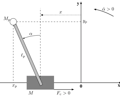
HE swing-up and stabilization of a single inverted pen-dulum (SIP) is a popular and challenging problem in nonlinear control theory. It is popular because the shape and dynamics of the SIP resemble many different real world systems, such as the ones in Fig. 1, thus the control methods used can be utilized in numerous applications. The challenge in controlling the SIP arises because the equations of motion governing the system are inherently nonlinear and because the upright position is an unstable equilibrium. Furthermore, the system is under-actuated as it has two degrees of freedom, one for the cart’s horizontal motion and one for the pendulum’s angular motion, but only the cart’s position is actuated, while the pendulum’s angular motion is indirectly controlled.

In a laboratory setting, there are two main types of SIP systems: the rotary pendulum system, and the pendulum on a cart system. The controllers for these two systems are similar, but they have different actuator dynamics. The greatest difference between the two systems is that the pendulum on a cart system has a finite track length that needs to be taken into account, especially during swing-up. This paper only focuses on the controllers for a cart pendulum system.

The SIP control problem is composed of two tasks: the first task is to swing-up the pendulum from its downward hanging

E. Kennedy is with the Department of Mathematics & Statistics, Hollins University, Roanoke, VA 24020; email: [email protected]

H. Tran is with the Department of Mathematics, North Carolina State University, Raleigh, NC 27695; email: [email protected]

Manuscript received 10/13/17.

position, and the second task is to stabilize the pendulum around the vertical upright position. These two tasks are usually accomplished using two separate controllers, however, there are a few existing control methodologies that can handle both tasks without having to switch controllers [1]. Our novel stabilization controller was previously published in [2] and [3]. We have also presented a swing-up controller in [4]. Here, we will expand on our previous work by including a more in-depth derivation and analysis, as well as two other swing-up controllers that led to the controller published in [4].

A. Existing Energy-Based Control Methods

One of the most popular control methods for swinging up the pendulum is where the control law is chosen such that the energy of the pendulum builds until reaching the upright equilibrium. This technique was originally proposed by Astrom and Furuta in 1996 at the13th_{International Federation} of Automatic Control World Congress [5]. Their revised paper that included the implementation of their method on a rotary pendulum was published in 2000 [6]. Later, the method was adapted for a cart-pendulum system by Angeli in [7], but without taking the finite length of the track into account. In [8]–[11] the use of energy based controllers for the pendulum on a cart system is discussed. Control methods that consider the length of the track are presented in [12] and [13].

Many of the published controllers have only been tested in simulations and not in real-time experiments [1]. As almost all simulations use a simplified model to represent the dynamics of the SIP, the observed experimental results are often very dif-ferent from the previously published simulation results. These simplified SIP models commonly used in simulations usually ignore the effects of friction, and often fail to incorporate some physical restrictions like the maximum deliverable voltage by the amplifier, the capacity of the DC motor that drives the cart, and the finite track length [14].

II. SYSTEMDYNAMICS

A. System Representation and Notations

(2)

Fig. 1. Inverted pendulum like systems.

0 x

y

Fc>0 M

x

yp Mp

xp `p

α

˙

α >0

Fig. 2. Single inverted pendulum diagram.

TABLE I

INVERTEDPENDULUMMODELPARAMETERS

Symbol Description Value

Mw Cart Weight Mass 0.37 kg

M Cart Mass with Extra Weight 0.57 +Mwkg

Jm Rotor Moment of Inertia 3.90E-007 kg.m2

Kg Planetary Gearbox Gear Ratio 3.71

rmp Motor Pinion Radius 6.35E-003 m

Beq Equivalent Viscous Damping Coefficient 5.4 N.m.s/rad

Mp Pendulum Mass 0.230 kg

`p Pendulum Length from Pivot to COG 0.3302 m

Ip Pendulum Moment of Inertia at its COG 7.88E-003 kg.m2

Bp Viscous Damping Coefficient 0.0024 N.m.s/rad

g Gravitational Constant 9.81 m/s2

Kt Motor Torque Constant 0.00767 N.m/A

Km Back-ElectroMotive-Force Constant 0.00767 V.s/rad

Rm Motor Armature Resistance 2.6Ω

B. Equations of Motion

Using Langrange’s method, we have previously showed [2], [14] that the second-order time derivatives of the position of

the cart, x, and the angle of the pendulum, α, are the two non-linear equations

¨

x= −(Ip+Mp`2p)Beqx˙−Mp`pcos(α)Bpα˙ −(M_p2`3_p+IpMp`p) sin(α) ˙α2+ (Ip+Mp`2p)Fc

+Mp2` 2

pgcos(α) sin(α)

!,

D(α)

(1)

and

¨

α= (M +Mp)Mpg`psin(α)−(M +Mp)Bp( ˙α) −M_p2`2_psin(α) cos(α) ( ˙α)2−Mp`pcos(α)Beq( ˙x)

+Mp`pcos(α)Fc

!,

D(α),

(2)

whereD(α) = (M+Mp)Ip+M Mp`2p+Mp2`2psin

2₍_α₎_{, and}_x andαare both functions oft. Furthermore, the driving force, Fc, generated by the DC motor acting on the cart through the motor pinion is considered to be the single input to the system. Since in our real-time implementation the input is equal to the cart’s DC motor voltage, Vm, we can use Kirchhoff’s voltage law and the physical properties of our system to convert the driving force,Fc, to voltage input by deriving the relationship

Fc=−

K2

gKtKm( ˙x(t)) Rmr2mp

+KgKtVm

Rmrmp

. (3)

III. CONTROLLERDESIGN

(3)

A. Pendulum’s Energy

The total energy,Ep, of the pendulum at it’s hinge is given by the sum of it’s rotational kinetic energy and it’s potential energy, so

Ep=

1 2Jpα˙

2₊_M

p`pg(cos(α)−1), (4) where Jp, the pendulum’s moment of inertia at it’s hinge is defined as

Jp=

Z 2`p

0

r2Mp

2`p

dr= 4

3Mp`

2

p. (5)

Our goal is to increase the energy of the pendulum until it reaches the upright position, which means that we must design a controller so that the condition

dEp

dt ≥0 (6)

is guaranteed. Differentiating (4) yields

dEp

dt =Jpα˙α¨−Mp`pgsin(α) ˙α

= 4 3Mp`

2

pα˙α¨−Mp`pgsin(α) ˙α.

(7)

As derived in [4] and [14], the two Lagrange’s equations for our system can be written as

M+Mp+

JmKg2

r2 mp

!

¨

x(t) +Mp`psin(α(t)) ˙α(t)2 −Mp`pcos(α(t)) ¨α(t) =Fc−Beqx˙(t),

(8)

and

−Mp`pcos(α(t))¨x(t) +

4 3Mp`

2

pα¨(t)−Mp`pgsin(α(t))

=−Bpα˙(t). (9)

Then, using (9) we can rewrite (7) as

dEp

dt =Mp`pα˙cos(α)¨x. (10)

It should be noted, that as is commonly done in swing-up control derivation, the effects of viscous damping at the pendulum axis have been ignored (i.e. set Bp = 0). This is acceptable becauseBp is very small and its effect is minor.

B. Converting to Voltage Input

In most swing-up derivations, the control input is taken to be the acceleration of the cart, x, but for our real-time¨

implementation the control input is defined to be the voltage applied to the cart Vm. Thus, we need to express x¨ in terms of Vm. We will do this by considering Newton’s second law of motion together with D’Alembert’s principle,

Mx¨+Fai=Fc−Beqx,˙ (11)

whereFaiis the armature rotational inertial force acting on the cart [15]. As seen at the motor pinion, Fai can be expressed as a function of the armature inertial torque,Tai, thus

Fai= KgTai

rmp

. (12)

Now, applying Newton’s second law of motion to the shaft of the cart’s DC motor yields

Jmθ¨m=Tai, (13)

where θm is the rotational angle of the motor shaft. Using the mechanical configuration of the cart’s rack-pinion system and the technical specifications from the Quanser IP02 User Manual [16], as well as the study of the electrodynamics of a DC motor in [17] we have

θm=

Kgx rmp

. (14)

Then, we can substitute equations (14) and (13) into (12) to obtain

Fai= K2

gJmx¨ rmp

. (15)

With the use of equations (3) and (15), we can express (11) as

M+K

2 gJm r2

mp

!

¨

x=− Beq+

K2 gKtKm Rmrmp2

!

˙

x+KgKtVm

Rmrmp .

(16) Solving forx¨ results in

¨

x=KgKtrmpVm−(K

2

gKtKm+BeqRmr2mp) ˙x Rm(M r2mp+Kg2Jm)

. (17)

Therefore, by substituting (17) into (10) and imposing the condition in (6), we obtain that our control input, Vm, must satisfy

dEp

dt =Mp`pα˙cos(α)

KgKtrmpVm Rm(M rmp2 +Kg2Jm) − (K

2

gKtKm+BeqRmrmp2 ) ˙x Rm(M rmp2 +Kg2Jm)

!

≥0.

(18)

C. Lyapunov Stability Condition

Consider the Lyapunov function

L(X) =1 2(Ep)

2

, (19)

which is defined to be zero when the pendulum is in it’s upright position, and positive everywhere else. Then, based on Lyapunov’s theorem, we must have

dL dt =Ep

dEp dt

=EpMp`pα˙cos(α)

_K

gKtrmpVm Rm(M r2mp+Kg2Jm) − (K

2

!

≤0.

(20)

Substituting the model parameter values provided in Table I into (20) and simplifying yields the condition

(4)

0.25

-0.25 0

x <0,x >˙ 0

sg(X) = 1

x >0,x >˙ 0

sg(X) = 1

x <0,x >˙ 0

sg(X) = 1

x >0,x >˙ 0

sg(X) =−1

x <0,x <˙ 0

sg(X) =−1

x >0,x <˙ 0

sg(X) =−1

x <0,x <˙ 0

sg(X) = 1

x >0,x <˙ 0

sg(X) =−1

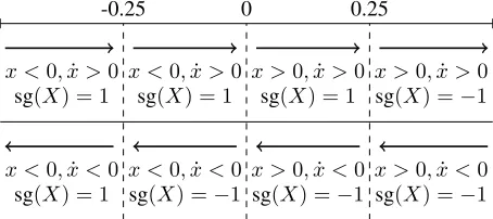
Fig. 3. Diagram representing how sg(X)is defined. The arrows indicate the direction of the cart’s displacement, while the number line indicates the cart’s position.

D. Control Law

Consider the control law of the form

Vm(X) =β|x|˙

−sign(Epα˙cos(α)) +sg(X)eη|x|

, (22)

where β and η are positive constants, sign represents the signum function, and the function sg(X)is defined as

sg(X) =0.5sign( ˙x)−sign(x)

−sign(|x| −0.25)(sign( ˙x) +sign(x)), (23)

which will output ±1 depending on the position of the cart and direction it is moving. Then, the sign of Vm will be the same as the sign of sg(X)because of the exponential term in (22). The total length of the track that the cart can travel is 0.814 m, indicating that the cart’s horizontal displacement in either direction must be less than 0.407 m (i.e. |x| <0.407

m). For safety reasons, the cart should not get too close to the end of the track, thus sg(X) was defined in such a way that it switches signs only when the cart’s displacement from the center is more than 0.25 m and the direction of the cart’s displacement is towards either track end. Fig. 3 provides a graphical representation of how sg(X)is defined. Substituting (22) into (21) gives

Epα˙cos(α)

β|x|˙ −sign(Epα˙cos(α)) +sg(X)eη|x|

−7.614 ˙x≤0, (24)

which can be rewritten as

β|x|˙ sg(X)Epα˙cos(α)eη|x|− |Epα˙cos(α)|

≤7.614 ˙xEpα˙cos(α). (25)

Then, dividing by |x||E˙ pα˙cos(α)|yields βsign(Epα˙cos(α))sg(X)eη|x|−1

≤7.614sign(Epα˙cos(α))sign( ˙x).

(26)

Physically for our system, a positive input voltage means positive cart displacement, therefore Vm andx˙ have the same sign. Furthermore, since we defined sg(X) to have the same sign as Vm, this also means that sg(X)andx˙ must also have the same sign. Now, consider the possible sign combinations for Epα˙cos(α)and sg:

• Case 1:Epα˙cos(α)>0 and sg(X) = 1 (x >˙ 0) βeη|x|−1≤7.614⇒β ≤ 7.614

eη|x|₋₁. • Case 2:Epα˙cos(α)>0 and sg(X) =−1(x <˙ 0)

β−eη|x|₋₁_{≤ −}₇_.₆₁₄_⇒_β_≥ 7.614

eη|x|_{+ 1}. • Case 3:Epα˙cos(α)<0 and sg(X) = 1 (x >˙ 0)

β−eη|x|₋₁_{≤ −}₇_.₆₁₄_⇒_β_≥ 7.614

eη|x|_{+ 1}. • Case 4:Epα˙cos(α)<0 and sg(X) =−1(x <˙ 0)

βeη|x|−1≤7.614⇒β ≤ 7.614 eη|x|₋₁.

Based on the above cases, we obtain thatβ andηmust satisfy the condition

7.614

eη|x|_{+ 1} ≤β≤

7.614

eη|x|₋₁. (27)

Moreover, we have to ensure that the commanded voltage does not make the power amplifier go into saturation, so we must design our control in a way that|Vm|<10Volts. This means that β andη also have to satisfy

β|x|˙ −sign(Epα˙cos(α)) +sg(X)eη|x|

≤10. (28)

Based on technical specifications provided in [16] we can calculate that the theoretical maximum velocity of the cart is

˙

x= 1.075m/s [14], which allows us to find a bound for (28) only in terms ofβandη. One particular, albeit arbitrary, choice forβ andη that satisfies all of the above conditions is β= 4

andη= 0.9. Both our simulation and real-time experimental results will be presented in the later sections of this paper, but first we consider two modifications to the control law given by equation (22).

IV. A MOREROBUSTSWING-UPCONTROLLER

A. Modified Lyapunov Function

Even though most publications on energy-based control methods for the swing-up of the pendulum use the same Lya-punov function we used in equation (19) for their derivation, in [18] Maeba et al. point out that this function has several zeros aside from the upright position. In fact, the pendulum’s energy given by (4), and thus the Lyapunov function in (19), is zero every time the pendulum’s angle and angular velocity satisfy

˙

α=±

s

3g(1−cos(α)) 2`p

. (29)

This means that the presented controller is not guaranteed to swing the pendulum up since the energy will stop building once the desired zero energy is achieved. To fix this problem, consider the Lyapunov function

L2(X) =

1 2E

2

(5)

(i.e. α = 0,α˙ = 0), and is strictly positive everywhere else. Differentiating (30) and utilizing (20) we obtain the new Lyapunov condition

dL2

dt =EpMp`pα˙cos(α)

KgKtrmpVm Rm(M rmp2 +Kg2Jm) − (K

2

!

+3

2kcos(α) sin(2α) ˙α

≤0.

(31)

Substituting the model parameter values provided in Table I into (31) yields the new condition

Epα˙cos(α)(Vm−7.614 ˙x) + 12.28kα˙cos(α) sin(2α)≤0, (32) that the control input, Vmmust satisfy.

B. Modified Control Law

Consider the control law of the form

Vm(X) =β1|x|˙

−β2sign(Epα˙cos(α)) +sg(X)eη|x|

−β3sign( ˙αcos(α))|sin(2α)| Ep

,

(33)

where β1, β3, andη are positive constants,1 > β2 >0, and sg is the same function defined in (23). Note that equation (33) is a modification of the previously presented control law in (22). Substituting (33) into (32) gives

Epα˙cos(α) β1|x|˙

−7.614 ˙x

!

−β3|α˙cos(α)||sin(2α)|

+ 12.28kα˙cos(α) sin(2α)

≤0.

(34)

The above inequality is satisfied when

Epα˙cos(α)

β1|x|˙

−7.614 ˙x≤0, (35)

and

−β3|α˙cos(α)||sin(2α)|+ 12.28kα˙cos(α) sin(2α)≤0 (36) are both satisfied. Based on our earlier conditions in (26) and (27), we can obtain that (35) holds when

7.614

eη|x|₊_β

2

≤β1≤

7.614

eη|x|₋_β

2

. (37)

Furthermore, inequality (36) is satisfied when

β3≥12.28k. (38)

In addition to the conditions (37) and (38), the sign of Vm should be given by the value of sg(X) to make sure the cart avoids the edges of the track. Therefore, we must have

sign β1|x|˙

!

=sg(X). (39)

Now, consider the possible sign combinations forEpα˙cos(α) and sg(X):

• Case 1:Epα˙cos(α)>0 and sg(X) = 1 (i.e. want Vm>0,x >˙ 0)

β1|x|˙

−β2+eη|x|

−β3|sin(2α)| |Ep|

>0

⇒β1>

β3|sin(2α)| |x||E˙ p|(eη|x|−β2)

.

• Case 2:Epα˙cos(α)>0 and sg(X) =−1 (i.e. want Vm<0,x <˙ 0)

β1|x|˙

−β2−eη|x|

−β3|sin(2α) |Ep|

<0

⇒β1>−

β3|sin(2α)| |x||E˙ p|(eη|x|+β2)

.

• Case 3:Epα˙cos(α)<0 and sg(X) = 1 (i.e. want Vm>0,x >˙ 0)

β1|x|˙

β2+eη|x|

+β3|sin(2α)|

|Ep|

>0

⇒β1>−

β3|sin(2α)| |x||E˙ p|(eη|x|+β2)

.

• Case 4:Epα˙cos(α)<0 and sg(X) =−1 (i.e. want Vm<0,x <˙ 0)

β1|x|˙

β2−eη|x|

+β3|sin(2α)|

|Ep|

<0

⇒β1>

β3|sin(2α)| |x||E˙ p|(eη|x|−β2)

.

The above cases all hold when the constantsβ1, β2, β3,andη satisfy

β1>

β3|sin(2α)| |x||E˙ p|(eη|x|−β2)

. (40)

To avoid division by zero and bound the value of β1, we can saturate the signals of Ep and x˙ so that |Ep| > δ1 and |x|˙ > δ2 for some small positive constantsδ1 andδ2. Then, the condition (40) will be satisfied when

β1≥

β3 δ1δ2(1−β2)

. (41)

(6)

V. INCORPORATINGVISCOUSDAMPING AT THE

PENDULUMAXIS

The two swing-up methods presented so far in the previous sections have accounted for viscous damping friction as seen at the cart’s motor pinion, but they have ignored the effects of viscous damping as seen at the pendulum axis. Though the effect of the viscous damping term, Bpα, in equation (9)˙ is small, it is desirable for real-time experiments and some applications to use a more complete model. In this section, we present another modification for our previous swing-up controllers to include viscous damping at the pendulum axis. If we include theBpα˙ term from (9), then equation (10) becomes

dEp

dt =Mp`pα˙cos(α)¨x−Bpα˙

2_, ₍₄₂₎

which can be rewritten as dEp

dt =Mp`pα˙cos(α)

_K

gKtrmpVm Rm(M r2mp+Kg2Jm) − (K

2

!

−Bpα˙2

(43)

using equation (17). Then, using the modified Lyapunov func-tion given in (30), and adding the viscous damping term into the derivate, we can modify (31) to obtain the new condition

dL2

dt =EpMp`pα˙cos(α)

_K

gKtrmpVm Rm(M rmp2 +Kg2Jm) − (K

2

!

+3

2kcos(α) sin(2α) ˙α− EpBpα˙

2

≤0.

(44)

Substituting the model parameter values provided in Table I into (44), and simplifying yields the condition

Epα˙cos(α)(Vm−7.614 ˙x) + 12.28kα˙cos(α) sin(2α) −0.0197Epα˙2≤0,

(45)

that our modified controller must satisfy to guarantee Lya-punov stability. To account for the effect of the damping term, consider the control law of the form

Vm(X) =β1|x|˙

+ 0.0197sign(Ep) ˙αcosα,

(46)

which is just a modification of (33) with positive constants, β1,β3,η, and 0 < β2 < 1. Substituting (46) into (45), and simplifying results in

Epα˙cos(α) β1|x|˙

−7.614 ˙x

!

−β3|α˙cos(α)||sin(2α)|

+ 12.28kα˙cos(α) sin(2α)−0.0197 sin2(α)|Ep|α˙2 ≤0.

(47)

As before, the inequality in (47) is satisfied when both (37) and (38) hold for the constants. Furthermore, we must make sure that sign(Vm(X)) =sg(X). Now, consider the possible sign combinations for Epα˙cos(α)and sg:

• Case 1:Epα˙cos(α)>0 and sg(X) = 1 (i.e. want Vm>0,x >˙ 0)

β1|x|˙

−β2+eη|x|

−β3|sin(2α)| |Ep|

+0.0197|α˙cosα|>0

⇒β1>

β3|sin(2α)| |x||E˙ p|(eη|x|−β2)

−0.0197|α˙cos(α)| |x|˙ (eη|x|₋_β

2)

• Case 2:Epα˙cos(α)>0 and sg(X) =−1 (i.e. want Vm<0,x <˙ 0)

β1|x|˙

−β2−eη|x|

−β3|sin(2α) |Ep|

+0.0197|α˙cosα|<0

⇒β1>−

β3|sin(2α)| |x||E˙ p|(eη|x|+β2)

+0.0197|α˙cos(α)|

|x|˙ (eη|x|₊_β

2) .

• Case 3:Epα˙cos(α)<0 and sg(X) = 1 (i.e. want Vm>0,x >˙ 0)

β1|x|˙

β2+eη|x|

+β3|sin(2α)|

|Ep| −0.0197sign(Ep) ˙αcosα >0

⇒β1>

0.0197|α˙cos(α)| |x|˙ (β2+eη|x|)

− β3|sin(2α)| |x||E˙ p| β2+eη|x|

.

• Case 4:Epα˙cos(α)<0 and sg(X) =−1 (i.e. want Vm<0,x <˙ 0)

β1|x|˙

β2−eη|x|

+β3|sin(2α)|

|Ep| −0.0197sign(Ep) ˙αcosα <0

⇒β1>

β3|sin(2α)| |x||E˙ p|(eη|x|−β2)

−0.0197|α˙cos(α)| |x|˙ (eη|x|₋_β

2) .

The above cases all hold when the constantsβ1, β2, β3,andη satisfy

β1>

β3|sin(2α)| |x||E˙ p|(eη|x|−β2)

−0.0197|α˙cos(α)| |x|˙ (eη|x|₋_β

2)

(48)

and

β1>

0.0197|α˙cos(α)| |x|˙ (β2+eη|x|)

− β3|sin(2α)| |x||E˙ p| β2+eη|x|

. (49)

(7)

VI. SIMULATIONRESULTS

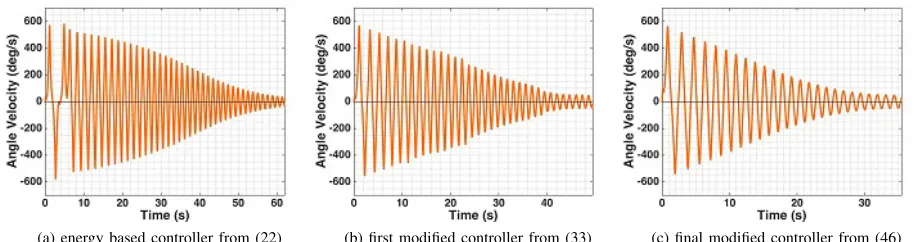
All three of the presented swing-up controllers were tested in simulation using Simulink in MATLAB. Since the starting downward position of the pendulum is a stable equilibrium we must input some initial voltage to get the experiment started. The starting voltage for our simulation was 8 Volts that was applied for 0.1 second. The resulting state responses are graphed in Figs. 4-7 with the corresponding control efforts presented in Fig. 8. The dashed blue lines in Fig. 5 indicate the region where the stabilization control can take over (i.e. where |α| <15◦) [14]. A numerical summary comparing the three simulations is given in Table II. For all three of the controllers the values of the states and the required control effort stayed within the possible ranges deliverable by the apparatus we use for real time experiments. Figure 4 indicates that the cart did not go past the end of the track in any of the simulations (i.e. the value of |x| stayed below 0.407 m). The original energy based controller from equation (22) was the slowest at swinging up the pendulum, taking approximately 55 seconds, followed by the first modified controller from equation(33), which took approximately 40 seconds. The final modified controller from equation (46) was by far the fastest at swinging up the pendulum, taking only 28 seconds. Furthermore, this final controller used the least amount of voltage on average (using only 0.68 Volts). The original energy based controller used 0.83 Volts on average, which is less than the average of 0.978 Volts used by the first modified controller.

VII. REAL-TIMEIMPLEMENTATION

A. Apparatus

The apparatus used in our real-time experiments was de-signed and provided by Quanser Consulting Inc. (119 Spy Court Markham, Ontario, L3R 5H6, Canada). This includes a single inverted pendulum mounted on an IP02 servo plant (depicted in Fig. 9), a VoltPAQ amplifier, and a Q2-USB DAQ control board. The IP02 cart incorporates a Faulhaber Coreless DC Motor (2338S006) coupled with a Faulhaber Planetary Gearhead Series 23/1. The cart is also equipped with a US Digital S1 single-ended optical shaft encoder. The detailed technical specifications can be found in [16]. A diagram of our experimental setup is included in Fig. 10.

B. Experimental Results

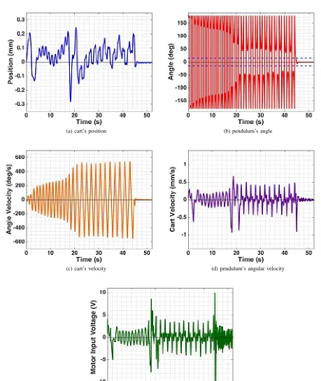
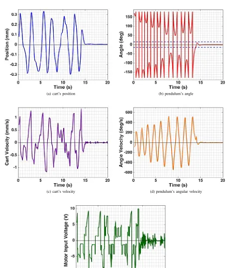
The original energy based controller from equation (22) and the final modified controller from equation (46) were both successfully implemented in real-time using Simulink and MATLAB with Quanser’s QuArc real-time control software. The real-time state response and the corresponding control effort are given in Fig. 11 for the original energy based controller from (22), and in Fig. 12 for the final modified controller from (46). A numerical summary comparing the real-time performance of these two controllers is given in Table III. The best swing-up time for the modified controller from (46) was only about 15 seconds, which is three times faster than our best swing-up time for the original energy based controller from (22). The 15 second swing-up time is

comparable to the swing-up time of the proportional-velocity controller provided by Quanser with our apparatus [19]. The modified controller used 2.89 Volts on average while the original controller only used only 1.35 Volts on average. For both controllers, the required control effort reached the upper limit of 10 Volts on one occasion and had to be saturated. Once the pendulum reached within15◦ of the upright position, our power series based stabilization controller presented in [2], [3] and [14] successfully took over.

We repeated the experiment with both controllers several times. Even though we have been able to achieve successful swing-up using the original energy based controller from (22), this has not been the case for every experimental run. There have been some instances when instead of swinging up to the upright position, the pendulum ended up swinging back and forth at a constant rate without building up more energy. This is most likely caused by the issue with the Lyapunov function that we discussed in Section IV. We did not experience this phenomena with our modified controller from (33), but we did observe a wide range of swing-up times ranging between 15 to 40 seconds for that controller. This inconsistency is likely caused by the way the function sg is defined. During the swing-up procedure the sg function causes the cart to make very fast big moves, and when the cart gets close to the end of the track the controller successfully makes the cart move away from the edge with a quick jerking movement. Unfortunately, when the pendulum is near the upright position, this fast jerk of the cart can overpower the movement of the pendulum, and make the pendulum lose momentum. Making up this loss of momentum increases the swing-up time [4], [14].

VIII. CONCLUSION

We have presented and successfully implemented a new energy-based swing-up controller that was derived using Lya-punov functions based on the method originally proposed by Astrom and Furuta [5], [6]. We’ve also provided two modi-fications to make the swing-up method more appropriate for real-time implementation. Our controller is based on a more complex dynamical model for the SIP system than the models that are most commonly used in the literature. In addition to considering the electrodynamics of the DC motor that drives the cart, we’ve also considered viscous damping friction as seen at the motor pinion, and our last modification also considered the viscous damping as seen at the pendulum axis. Furthermore, we have accounted for the limitation of having a cart-pendulum system with a finite track length. This was accomplished using a method that is different from previously published methods of others. Our final swing-up controller, given in equation (46), was able to swing the pendulum up in approximately 15 seconds. However, the swing-up time of our final controller is inconsistent.

REFERENCES

(8)

(a) energy based controller from (22) (b) first modified controller from (33) (c) final modified controller from (46) Fig. 4. Simulated state response of the cart’s position.

(a) energy based controller from (22) (b) first modified controller from (33) (c) final modified controller from (46) Fig. 5. Simulated state response of the pendulum’s angle.

(a) energy based controller from (22) (b) first modified controller from (33) (c) final modified controller from (46) Fig. 6. Simulated state response of the cart’s velocity.

(9)

(a) energy based controller from (22) (b) first modified controller from (33) (c) final modified controller from (46) Fig. 8. Simulated control effort.

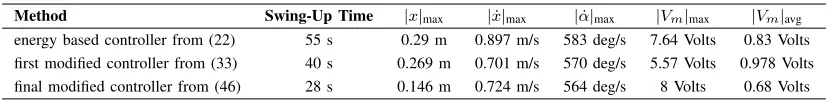
TABLE II

SUMMARY OFSIMULATEDSTATERESPONSE ANDCONTROLEFFORT

Method Swing-Up Time |x|max |x˙|max |α˙|max |Vm|max |Vm|avg

energy based controller from (22) 55 s 0.29 m 0.897 m/s 583 deg/s 7.64 Volts 0.83 Volts first modified controller from (33) 40 s 0.269 m 0.701 m/s 570 deg/s 5.57 Volts 0.978 Volts final modified controller from (46) 28 s 0.146 m 0.724 m/s 564 deg/s 8 Volts 0.68 Volts

TABLE III

SUMMARY OFEXPERIMENTALSTATERESPONSE ANDCONTROLEFFORT

Method Best Swing-Up Time |x|max |x˙|max |α˙|max |Vm|max |Vm|avg

energy based controller from (22) 45 s 0.281 m 0.936 m/s 554 deg/s 10 Volts 1.35 Volts final modified controller from (46) 15 s 0.335 m 1.36 m/s 547 deg/s 10 Volts 2.89 Volts

Fig. 9. Single inverted pendulum mounted on a Quanser IP02 servo plant.

[2] E. Kennedy and H. Tran, “Real-time implementation of a power series based nonlinear controller for the balance of a single inverted pendulum,” inProceedings of The International MultiConference of Engineers and Computer Scientists 2015 Vol I, IMECS 2015, Hong Kong, 18-20 March 2015, pp. 237–241, ISBN: 978–988–19 253–2–9, ISSN: 2078–0958 (Print); ISSN: 2078–0966 (Online).

[3] E. A. Kennedy and H. T. Tran, Transactions on Engineering Tech-nologies, Int. MultiConference of Engineers and Computer Scientists. Springer, 2016, ch. Real-Time Stabilization of a Single Inverted Pendu-lum Using a Power Series Based Controller.

[4] E. Kennedy and H. Tran, “Swing-up of an inverted pendulum on a cart using a modified energy based approach,” in Lecture Notes in Engineering and Computer Science: Proceedings of The International MultiConference of Engineers and Computer Scientists 2016, IMECS 2016, Hong Kong, 16-18 March 2016, pp. 185–190, ISBN: 978–988–

IP02

Amplifier

DAQ

Computer

Control Signal

Pendulum Angle & Cart Position Cart Encoder

Pendulum Encoder

Amplifier Command Motor Connector

Fig. 10. Diagram of experimental setup.

19 253–8–1, ISSN: 2078–0958 (Print); ISSN: 2078–0966 (Online). [5] K. J. Astrom and K. Furuta, “Swinging up a pendulum by energy

control,” in Prepints of the 13th IFAC World Congress, vol. E, San Francisco, CA, 1996, pp. 37–42.

[6] ——, “Swinging up a pendulum by energy control,”Automatica, vol. 36, pp. 287–295, 2000.

[7] D. Angeli, “Almost global stabilization of the inverted pendulum via continuous state feedback,”Automatica, vol. 37, pp. 1103–1108, 2001. [8] C. C. Chung and J. Hauser, “Nonlinear control of a swinging pendulum,”

Automatica, vol. 31, no. 6, pp. 851–862, 1995.

[9] R. Lozano, I. Fantoni, and D. J. Block, “Stabilization of the inverted pendulum around its homoclinic orbit,” Systems & Control Letters, vol. 40, pp. 197–204, 2000.

[10] A. Siuka and M. Schoberl, “Applications of energy based control methods for the inverted pendulum on a cart,”Robotics and Autonomous Systems, vol. 57, pp. 1012–1017, 2009.

(10)

(a) cart’s position (b) pendulum’s angle

(c) cart’s velocity (d) pendulum’s angular velocity

(e) control effort

(11)

(a) cart’s position (b) pendulum’s angle

(c) cart’s velocity (d) pendulum’s angular velocity

(e) control effort

(12)

& Control Letters, vol. 47, pp. 355–364, 2002.

[13] C. Huifeng, L. Hongxing, and Y. Peipei, “Swing-up and stabilization of the inverted pendulum by energy well and sdre,” in Control and Decision Conference, 2009. CCDC ’09. Chinese. IEEE, June 2009, pp. 2222–2226.

[14] E. Kennedy, “Swing-up and stabilization of a single inverted pendulum: Real-time implementation,” Ph.D. dissertation, North Carolina State University, 2015. [Online]. Available: http://www.lib.ncsu.edu/resolver/ 1840.16/10416

[15] Linear Motion Servo Plants: IP01 or IP02 - Linear Experiment #1: PV Position Control - Student Handout, 4th ed., Quanser Consulting, Inc. [16] Linear Motion Servo Plants: IP01 or IP02 - IP01 and IP02 User

Manual, 5th ed., Quanser Consulting, Inc.

[17] T. P. Pavlic, “Rotary electrodynamics of a dc motor: Motor as mechan-ical capacitor,” 2007-2009, eCE 758: Control System Implementation Laboratory Notes, Department of Electrical and Computer Engineering, The Ohio State University.

[18] T. Maeba, M. Deng, A. Yanou, and T. Henmi, “Swing-up controller design for inverted pendulum using energy method based on lyapunov functions,” in Proceedings of the 2010 International Conference on Modelling, Identification and Control, Okayama, Japan, July 2010, pp. 768–773.

[19] Linear Motion Servo Plant: IP02 - Linear Experiment #6: PV and LQR Control - Student Handout, 4th ed., Quanser Consulting, Inc.

Emese Kennedywas born in Budapest, Hungary. She received the B.A. in mathematics from Skid-more College in 2010, and the M.S. and Ph.D. degrees in applied mathematics from North Carolina State University in 2013 and 2015, respectively. She is currently a Visiting Assistant Professor of Mathematics at Hollins University in Roanoke, VA.