Spatial Dnamics of Infection by Multiple Pathogens: A Case Study with Yellow Dwarf Virus.

(1)

Abstract

LYZINSKI, REBECCA ANNE. Spatial Dynamics of Infection by Multiple Pathogens: A Case Study with Yellow Dwarf Viruses. (Under the direction of Dr. Kevin Gross.)

Mathematical models are useful tools for understanding disease dynamics, but often

assume a “well-mixed” population. In reality, populations usually violate this

assumption, exhibiting heterogeneous mixing. Spatial structure is one mechanism that

creates heterogeneous mixing by limiting the number of possible contacts. One-pathogen

models show that inclusion of spatial structure decreases the prevalence of infection. In

this paper, we extend spatial models to a two-pathogen system based on cereal and barley

yellow dwarf viruses (C/BYDVs). By comparing the spatial model to a nonspatial

model, we can determine how prevalence of coinfection and single infection changes

with localized pathogen transmission. The model predicts that when pathogens do not

interact within hosts, coinfection decreases as pathogen transmission becomes

increasingly localized. Spatial aggregation of the pathogens explains this result. We also

examine a model with decreased transmission due to cross-protection, a model with

increased transmission due to synergism, and a model with increased host mortality due

to synergism. Most notably, when hosts infected by multiple pathogens experience

greater mortality than singly infected hosts, localized pathogen transmission makes

pathogen persistence more likely. Thus, these models predict that overall pathogen

(2)

Spatial Dynamics of Infection by Multiple Pathogens: A Case Study with Yellow Dwarf Viruses

by

Rebecca Anne Lyzinski

A thesis submitted to the Graduate Faculty of North Carolina State University

in partial fulfillment of the requirements for the Degree of

Master of Science

Biomathematics

Raleigh, North Carolina

2011

APPROVED BY:

_______________________________ ______________________________

Dr. Alun Lloyd Dr. Charles Mitchell

________________________________ Dr. Kevin Gross

(3)

Biography

Rebecca was raised in northern Virginia, where she graduated from Oakton High School

in 2004. She proceeded to St. Mary’s College of Maryland where she began as a

psychology major. Quickly she learned that her true passions were mathematics and

biology. After her junior year of college, Rebecca participated in a mathematical biology

Research Experience for Undergraduates at Penn State Erie, The Behrend College. The

internship opened up to her the world of research in mathematical modeling and taught

her about graduate programs in biomathematics. After graduating from St. Mary’s

College of Maryland with a double major in mathematics and biology, Rebecca

continued to North Carolina State University where she received a Masters of Science

(4)

Acknowledgements

I would like to thank my graduate research advisor Dr. Kevin Gross for all his time,

patience, dedication, and expertise. I would also like to thank my committee members,

Dr. Alun Lloyd and Dr. Charles Mitchell, for their help and support. In addition, I want

to thank my undergraduate advisor, Dr. Samantha Elliott, for giving so much of her time

and support even after I graduated. I would also like to thank Dr. Michael Rutter and the

mathematical biology REU at Penn State Erie for introducing me to biomathematics.

I would also like to thank my family and friends for all their support. In particular, I

would like to thank my parents who have always supported me in whatever I wanted to

do and my brother who always helped me to find the fun in things. Without all their love

and support, I never would have made it this far. I would also like to thank all my friends

from North Carolina State University, St. Mary’s College of Maryland, Intervarsity

Graduate Christian Fellowship, and Edenton Street United Methodist Church for all their

(5)

List of Tables

(8)

List of Figures

Figure 1. Barley yellow dwarf virus model...13

Figure 2. Spatial structure of neighbors (n) around a single host individual (X)...17

Figure 3. Deterministic ODE model fixed points and stochastic nonspatial model means for the baseline model ...25

Figure 4. The mean prevalence of infection for the baseline model ...28

Figure 5. Aggregation of pathogen A...31

Figure 6. Map of the lattice to show aggregation in the baseline model...32

Figure 7. The mean prevalence of infection for the cross-protection model...34

Figure 8. The mean prevalence of infection for the increased transmission model...37

Figure 9. The mean prevalence of infection for the increased mortality model...40

Figure 10. Aggregation of pathogen A in the increased mortality model...42

(9)

Introduction

1. Overview

Mathematical models are useful tools for understanding disease dynamics. They

allow us to explore questions about topics such as pathogen transmission, virulence,

disease prevalence, and infectiousness. The classic epidemic models function on the

assumption of a “well-mixed” population in which all individuals are equally likely to

come into contact with each other (Bailey 1975; Boylan 1991; Brauer 2008; Brown and

Bolker 2004; Lefevre 1983). However, real populations often violate this assumption

through individual differences, such as differences in susceptibility, infectiousness,

behaviors, and number of contacts (Brauer 2008; Boylan 1991; Lefevre 1983). Here, we

will focus on the effects of spatial structure created by heterogeneous mixing.

The spatial structure of a host population affects the dynamics of diseases spread

through contact. When spatial structure is considered, the path of the disease becomes

limited. Hosts close to an infected individual are at high risk for infection whereas hosts

far away have little chance of becoming infected (Tildesley et al. 2010). This limits the

number of susceptible hosts that the disease can reach, affecting the total number of

individuals that could potentially become infected (Brown and Bolker 2004; Keeling

1999; Tildesley et al. 2010). To explore the extent to which spatial structure changes

disease dynamics, epidemic models can be used to make comparisons between a spatial

(10)

Mathematical models for one-pathogen systems have provided a good basis for

studying the differences between spatial and nonspatial structures, but multiple pathogens

are often capable of inhabiting a single host organism at the same time, creating a more

complex system (Seabloom et al. 2009). This system adds pathogen interactions as a

factor in determining disease dynamics, which brings up new questions. Can the

pathogens coexist and under what conditions? Does the presence of multiple pathogens

increase infection prevalence? Does the presence of multiple pathogens increase host

mortality? These are only some of the questions of concern for a system with multiple

pathogens.

These questions arise in many biological systems, including the system involving

cereal and barley yellow dwarf viruses (C/BYDVs) and the host plants infected by

C/BYDVs. C/BYDVs exist as at least five different species, which can coinfect grasses in

the family Poaceae including cereal crops like barley and wheat (Miller and Rasochova

1997; D’Arcy 1995). Depending on the combination, C/BYDV species exhibit cross

protection, where one pathogen prevents infection by another, and synergism, where

pathogen interaction increases transmission or virulence (Miller and Rasochova 1997).

Some symptoms of C/BYDVs include growth reduction, yellowing, and sterility, which

can lead to yield reduction and significant agricultural losses (Miller and Rasochova

1997; Jensen and D’Arcy 1995; Lister and Ranieri 1995). C/BYDVs are obligately

transmitted by both winged and wingless aphids (Halbert and Voegtlin 1995; Seabloom

(11)

limited movement of wingless aphids while a nonspatial model can describe the wider

range of movement by winged aphids (Chaussalet et al. 2000).

In this paper, we will focus on exploring the effect of spatial structure on

coinfection dynamics by using extensions of the well-known susceptible-infected (SI)

model. Specifically, we will apply a two-pathogen, one-host model to C/BYDVs to ask

the following questions. 1. Does spatial structure affect the number of coinfected hosts

relative to a well-mixed population? 2. Could pathogen clustering in the spatial model be

responsible for a change in the number of coinfected hosts? 3. How does spatial structure

affect disease dynamics when pathogens exhibit cross-protection, that is, when infection

by one pathogen reduces the possibility of infection by a second pathogen? 4. How does

spatial structure affect disease dynamics when pathogens exhibit synergism in the form of

increased transmission? 5. How does spatial structure affect disease dynamics when

pathogens exhibit synergism in the form of increased mortality? We will explore each of

these questions with mathematical models and computer simulations.

2. Mathematical Tools for Analyzing Nonspatial and Spatial Models

Many mathematical models assume a “well-mixed” population, making them

simpler and easier to analyze. However, most real populations do not follow this

assumption, so the methods for analyzing nonspatial models are being expanded to assess

more complicated spatial models. Here we discuss some of the mathematical tools used

(12)

2.1 Tools for Nonspatial Models

A deterministic ordinary differential equation (ODE) model is one of the simplest

methods for analyzing disease dynamics under the assumption of a “well-mixed”

population. The ordinary differential equations can be analyzed to give us information

about the number of individuals in each state, the stability of the infection, the possibility

of an outbreak, and more (Kermack and McKendrick 1932). However, an ODE model

always gives the same results for a given set of initial conditions, which is unrealistic for

an actual population. Real populations usually exhibit more variation than these

deterministic models account for, so these models can be expanded to include stochastic

events.

Stochastic nonspatial models for epidemics are commonly analyzed in two ways,

through simulations and analytical tools (Dangerfield et al. 2009). Simulations of

stochastic nonspatial models typically use Markov processes and the memoryless

property to create a random walk in the number of individuals in each state (Ross 2007;

Keeling and Ross 2008). These simulations are usually run using computer programs

designed for numerical analysis. More analytical approaches to exploring the behavior of

stochastic nonspatial models include exact Kolmogorov forward equations for

determining the probabilities of each state and diffusion approximations for determining

the proportion of individuals in each state and the variability of the system (Keeling and

(13)

2.2 Tools for Spatial Models

Similar to stochastic nonspatial models, stochastic spatial models can be analyzed

through either simulations or analytical methods, but these tools become more difficult to

use without the assumption of a “well-mixed” population. Computer simulations can

expand upon the methods used in stochastic nonspatial models to include spatial

structure. These simulations obtain the number of infected individuals over time as

determined by a stochastic spatial model (Chaussalet et al. 2000; Keeling 1999). The

analytical method of pairwise approximations also determines the approximate number of

infected individuals for a stochastic spatial model by taking into account the number of

pairs and type of pairs in the system (Dangerfield et al. 2009). Moment closure analysis

provides another approximation approach for exploring disease dynamics in spatial

systems through the use of differential equations (Brown and Bolker 2004). In this paper,

we will focus on the use of simulations to explore disease dynamics for both a stochastic

nonspatial model and a stochastic spatial model.

3. Spatial Structure in One-Pathogen Models

Epidemic models for a one-pathogen system set the groundwork for

understanding the difference in disease dynamics between a spatial and a nonspatial

structure. A susceptible-infected-recovered (SIR) model shows that the total number of

hosts infected during an epidemic is smaller for a spatial network model than for a

(14)

possible contacts in a spatial model. In spatial models a host can only infect its

neighbors, the number of neighbors being determined by the connectivity level. Once all

of the neighbors are infected, the original infected host no longer has susceptible hosts to

spread the pathogen to, so the epidemic is slowed (Tildesley et al. 2010, Brown and

Bolker 2004). Moment-closure analysis confirms that epidemics become slowed with the

addition of spatial structure (Brown and Bolker 2004). The slowed epidemic spread can

also be explained through susceptible-infected-susceptible (SIS) model extensions, which

have shown that the limited contact structure of a spatial model results in lower

transmission rates (Boots and Sasaki 1999). This occurs because small spatial

neighborhoods limit resource availability to only a few hosts, creating the greatest

intraspecific competition for pathogens (Keeling 1999). In addition to there being fewer

infected hosts in a spatial model, SIS models together with pairwise approximations show

that spatial structure produces a small increase in the variation of the number of infected

hosts. This increase becomes more apparent for small neighborhood sizes combined with

low levels of infection (Dangerfield et al. 2009). Understanding these results for a

one-pathogen system provides the foundation for expansion to more complex systems.

4. Two-Pathogen Models

Two-pathogen SIS models provide a good starting place for exploring the new

questions that arise with interactions among multiple pathogens. May and Nowak were

among the first to define some of these interactions and create mathematical models that

(15)

within host pathogen interactions: superinfection and coinfection (May and Nowak 1995;

Nowak and May 1994). These extremes are important to understand as they may give

insight to the more complicated scenarios that lie in between superinfection and

coinfection (May and Nowak 1995).

Superinfection occurs when competition between two pathogens drives out the

less virulent pathogen, replacing it with the more virulent pathogen. In this case, only the

more virulent pathogen is transmitted. Adding superinfection to an epidemic model

decreases the number of infected hosts, increases the average virulence level, and

decreases the rate of transmission (Nowak and May 1994). The addition of spatial

structure to a superinfection model decreases virulence and the number of infected hosts

even more while increasing the possibility of strain replacement and extinction (Nunes et

al. 2006; Caraco et al. 2006).

The other type of within host pathogen interaction is coinfection, which will be

the focus of this paper. Unlike superinfection where one pathogen drives another

pathogen out of the host, coinfection occurs when multiple pathogens are able to stably

coexist within a host (May and Nowak 1995). This definition can also be expanded to

the broader definition of multiple pathogens infecting the same host at the same time

(Seabloom et al. 2009). In this case, all pathogens within the host can be transmitted to

another host (May and Nowak 1995). The results of epidemic models incorporating

coinfection depend on how the pathogens interact. In this paper we will consider three

(16)

4.1 Pathogen Interactions

When coinfection occurs with no interaction between the pathogens, transmission

rates for each pathogen remain unchanged. The only difference assumed by a

mathematical model is that a coinfected host acquires the death rate associated with the

most virulent pathogen (May and Nowak 1995). Coinfection under the no interaction

scenario can be explored using neutral null models, which model the dynamics of

indistinguishable pathogens by allowing both pathogens to stay at their initial conditions

rather than coming together at the same stable equilibrium (Lipsitch et al. 2009).

Cross protection, another type of pathogen interaction, occurs when one pathogen

already present within the host prevents another pathogen from infecting the host (Zhang

and Holt 2001). Especially in plants, this pathogen-provided immunity often occurs

because the resident pathogen triggers resistance pathways within the host, which can

provide protection against a variety of other pathogens (Barrett et al. 2009). With

increased resistance to infection, cross protection models result in a decrease in

coinfection prevalence and transmission rates. In some cases, cross protection has also

been shown through epidemic models to decrease overall infection prevalence (Seabloom

et al. 2009).

Synergism, a third type of pathogen interaction, arises when two pathogens

infecting the same organism lead to an increase in virus replication, virulence, and/or

transmission rate (Zhang et al. 2001). In plants, synergism can occur when one pathogen

(17)

defense (Barrett et al. 2009). When synergism leads to increased host mortality,

coinfection levels decrease. With substantial increases in synergistic mortality, overall

infection prevalence decreases (Seabloom et al. 2009). All of these coinfection processes

can be modeled using SIS model extensions (Lipsitch et al. 2009; Zhang and Holt 2001;

Zhang et al. 2001). However, little research has been conducted on using these SIS

(18)

Methods

1. Models and Their Architecture

In this paper, we consider three one-host, two-pathogen models: a nonspatial

ODE model, a stochastic nonspatial model, and a stochastic spatial model. The

nonspatial ODE model allows us to achieve a basic understanding of the system. The

stochastic nonspatial model allows us to expand upon the ODE model to incorporate

variation to capture the random events of real populations. Lastly, the stochastic spatial

model allows us to explore disease dynamics without the assumption of a “well-mixed”

population.

1.1 Nonspatial ODE Model

To explore C/BYDV dynamics, we use a one-host, two-pathogen SI model that

assumes the pathogens are indistinguishable and includes the potential for coinfection

(Bailey 1975; Kermack and McKendrick 1932; Lipsitch 2009). We assume the two

pathogens, labeled here as A and B, are indistinguishable to simplify our model. This

assumption allows for transmission and virulence rates to be the same for both pathogens,

reducing the number of parameters needed. Our model envisions a landscape of N

distinct patches, each of which can either be vacant or occupied by a single host. Hosts

can be uninfected (‘susceptible’), infected by one pathogen, or infected by both

pathogens. In total, our model includes five host states: vacant, susceptible, infected by

(19)

represented by V, S, IA, IB, and IX, respectively and can be described by the following

differential equations.

€

˙

S =α(S+φ1IA +φ1IB +φ2IX)(N−S−IA −IB −IX)

N −ν0S−λAS−λBS

˙

I _A =λAS−ν1IA −kλBIA ˙

I _B =λ_BS−ν₁I_B −kλ_AI_B

˙

I _X =kλ_BI_A +kλ_AI_B −(ν₁+ν₂)I_X

In these equations, N represents the total number of hosts and vacant patches (N =

V+S+IA+IB+IX) and is considered a constant term. This allows us to reduce the necessary

number of differential equations from five to four by rewriting the number of vacant

patches (V) as N-S-IA-IB-IX.

The transmission rates

€

λA and

€

λB quantify the rate at which susceptible hosts

become infected with pathogen A or pathogen B, respectively. These rates are the

product of a transmission rate constant,

€

β, and the number of infected hosts capable of

spreading the pathogen of interest, written as

€

λA =β(

I_A

N +

qI_X

N )

λ_B =β(IB

N +

qI_X

N )

€

β is assumed to be the same for both pathogens. The transmission rates include both

singly infected and coinfected hosts, because both can spread the pathogen to a

(20)

a singly infected host, so coinfected hosts are weighted by the parameter

€

q. In the

transmission rate equations, the number of infected hosts is represented as a proportion of

the total number of hosts and vacant patches.

These transmission rates can also be used to describe the rate at which a singly

infected individual becomes infected by a second pathogen. The rate at which a singly

infected host is infected by the other pathogen to become coinfected can be determined

by multiplying

€

λA and

€

λB by the parameter

€

k. Using

€

k allows the coinfection

transmission rate to be different from the single infection transmission rate. Once

transmission occurs and a host becomes either singly infected or coinfected, the host

never recovers, just as a plant infected with C/BYDV never recovers.

Our model includes host births and deaths. Both susceptible and infected hosts

produce offspring at a rate

€

α. Offspring can only be born into a vacant patch and the

new host always starts as a susceptible individual, because C/BYDV is not transmitted

vertically.

€

φ1 and

€

φ2 allow the number of offspring contributed by singly infected hosts

and coinfected hosts, respectively, to differ from the number of offspring produced by

healthy, susceptible hosts. We assume

€

φ2≤φ1≤1 , because infection by C/BYDV can

decrease fecundity (Seabloom 2009).

In addition to a birth rate, our model also has a death rate corresponding to each

type of host. Susceptible hosts die naturally at a rate

€

ν0. When a host becomes infected

(21)

infected by A and hosts infected by B is the same, because pathogens are assumed to be

indistinguishable. A coinfected host has at least the same death rate as a singly infected

host, but can have a higher death rate by adding the parameter

€

ν2≥0 to

€

ν1. Once a host

of any kind dies, the patch occupied by that host becomes vacant. All these transmission,

birth, and death rates allow for a total of nine possible state changes (Figure 1).

Figure 1. Cereal and barley yellow dwarf viruses model. The rates given here are per capita rates. V represents vacant patches. S represents susceptible hosts. IA represents

hosts infected by pathogen A. IB represents hosts infected by B. IX represents coinfected

hosts.

€

(22)

1.2 Stochastic Models

Here we analyze two stochastic models: a nonspatial model and a spatial model.

The dynamics of C/BYDVs spread by winged aphids is well represented by a nonspatial

model while a spatial model better represents the dynamics of C/BYDVs spread by

wingless aphids. By comparing the two models, we can reach a better understanding of

how C/BYDVs are spread in real populations.

1.2.1 Stochastic Nonspatial Model

The stochastic nonspatial model is very similar to the nonspatial ODE model. For

both models, the rates are the same as given by the arrows in Figure 1. Both the ODE

and stochastic nonspatial models also multiply the rates by the total number of

individuals in the state of interest. For example, the forces of infection

€

λA and

€

λB are

multiplied by the total number of susceptible individuals. This occurs because the

stochastic nonspatial model functions under the assumption that the population is

“well-mixed.” As long as one individual in the population is infected by a pathogen, then any

susceptible individual in the population can become infected by that pathogen. For

coinfection, as long as both pathogens are present somewhere in the population, then any

singly infected individual can become coinfected.

The stochastic nonspatial model functions as a continuous-time Markov model

where the state space of the model is the number of S, IA, IB, and IX individuals present at

(23)

the transition rates as given by Table 1, where [.] denotes the “concentration” in a given

‘neighborhood’. Each concentration is defined as the number of hosts in that state

divided by the neighborhood size, such as [S] = S/N. For the nonspatial model, the ‘neighborhood’ is the entire lattice. Therefore, the overall rates depend on the total

number of individuals in each state. In this case, N is the total number of individuals and vacant patches. A more extensive description of the algorithm used for this model can be

found in Section 3 of the Methods.

Table 1. Stochastic model events and rates where [.] denotes the “concentration”.

Event Rate

V  S

€€

α([S]+φ1[IA]+φ1[IB]+φ2[IX])

S  V

€

ν0

S  IA

€

λA=β([IA]+q[IX])

S  IB

€

λB=β([IB]+q[IX])

IA V

€

ν1 IA IX

€

kλB =kβ([IB]+q[IX])

IB V

€

ν1 IB IX

€

kλA =kβ([IA]+q[IX])

IX V

€

(24)

  1.2.2 Stochastic Spatial Model

Unlike the stochastic nonspatial model, the stochastic spatial model does not

assume that the population is “well-mixed”. This means that instead of using the total

number of individuals in a certain state, we only consider the individuals within a given

neighborhood size. In the spatial model, individuals are distributed on a square lattice

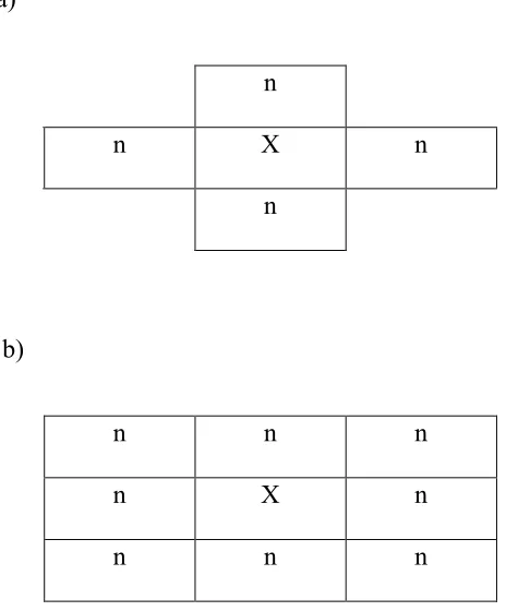
and each individual in the lattice has a neighborhood around it of n other individuals. Here we examine two neighborhood sizes: n=4 and n=8. For a neighborhood size of n=4, each individual has one neighbor above, one below, one to the left, and one to the right

(Figure 2a). For a neighborhood size of n=8, each individual has the same neighbors as in the n=4 model, but with the addition of the neighbors on the diagonals (Figure 2b). For both neighborhood sizes, the edges of the lattice wrap around so that each individual

has a complete neighborhood. For example, the individuals on the top row of the lattice

have a neighbor on the bottom row of the lattice and vice versa. Similarly, the

individuals in the left-most column of the lattice have a neighbor in the right-most

column and vice versa. The neighbors of an individual determine whether or not an

individual can become infected or coinfected. If the individual is susceptible then it can

only become infected if one of its neighbors is infected. If the individual is singly

infected with one pathogen, it can only become coinfected if one of its neighbors is

(25)

a)

n

n X n

n

b)

n n n

n X n

n n n

Figure 2. Spatial structure of neighbors (n) around a single host individual (X). (a) A neighborhood size of n=4. (b) A neighborhood size of n=8.

Similar to the stochastic nonspatial model, the stochastic spatial model is a

continuous-time Markov model. The state space for the spatial model is every possible

configuration of V, S, IA, IB, and IX individuals on the lattice. This model is also

event-driven with events occurring singly as determined by the transition rates given by Table

1. The overall rates only take into account the state of the neighbors of the chosen cell.

This means that where there is an S, IA, IB, or IX in the rate equations only the number of

neighbors in that state is counted not the total number of individuals in that state. With

(26)

number of individuals and vacant patches. A more extensive description of the algorithm

used for this model can be found in section 3 of the methods.

2. Biological Scenarios and Parameter Values

We start with a set of baseline conditions to represent no pathogen interaction and

then extend this case to incorporate three different variations. For the baseline model and

the three extensions, all parameters other than

€

k and

€

ν2 remain the same. To allow the

pathogen to persist, the death rate needs to be less than the transmission rate (

€

ν <β), so

we fix

€

β =1 and keep all the

€

ν parameters less than one. In exploring each type of

model, we allow

€

ν1 to vary and keep

€

ν0 constant. To determine the value of

€

ν0 we

would like to use, we look into a simpler model for insight. In a model that includes only

vacant patches and susceptible hosts, the equilibrium number of susceptibles is

€

1−ν0 α . If

we fix

€

α=1, then setting

€

ν0 =0.1 allows ninety percent of the population to be

susceptible and ten percent to be vacant patches. Based on this calculation, we use these

parameter values for

€

α and

€

ν0 in our model.

The rest of the parameters we determined based on assumptions. For simplicity,

we assume that hosts infected by one or both pathogens do not experience a change in

fecundity, so we set

€

φ1=φ2 =1. With the assumption that the pathogens are

indistinguishable, we set

€

(27)

equals the infectivity of singly infected hosts. In all these models, we set the total

number of patches equal to

€

N=2500.

2.1 Baseline

We start our exploration of spatial effects on coinfection with a baseline model

that assumes no pathogen interactions and then extend this model to incorporate pathogen

interactions. In the baseline model, the properties of the pathogens remain unchanged in

the presence of each other. To keep the transmission rate unchanged, we set

€

k=1 so that

the rate at which a singly infected host is infected by the second pathogen to become

coinfected remains the same as the rate at which a susceptible host is infected by either

pathogen A or pathogen B. We also assume

€

ν2=0 so that there is no change in the death

rate when both pathogens are present. The baseline model allows us to understand the

basic system and make comparisons to models with pathogen interaction.

2.2 Variations

2.2.1 Cross Protection

Some species of C/BYDVs exhibit cross protection, resulting in decreased

transmission (Seabloom et al. 2009). Typically this occurs between two closely related

(28)

  2.2.2 Synergism – Increased Transmission

For C/BYDVs, synergism usually occurs when two dissimilar species are present

(Miller and Rasochova 1997). One result of synergism between two species of

C/BYDVs is an increase in transmission (Seabloom 2009). This type of interaction is

represented in the model by setting k >1, increasing the transmission rate from single infection to coinfection.

2.2.3 Synergism – Increased Mortality

Synergism can also increase the mortality of a coinfected host due to interactions

between the pathogens (Zhang et al. 2001). In this case, we assume that the mortality

rate of a coinfected host is the sum of the mortality rates of the two types of singly

infected hosts. For our model the pathogens inflict the same mortality rates upon their

hosts, so we set

€

ν2=ν1.

3. Simulation Details for Stochastic Models

3.1 Description of the Algorithm

Both the stochastic nonspatial and stochastic spatial models are continuous-time

Markov models. The random variables that determine the processes of the

continuous-time Markov model depend on the rates, which we will represent here by

€

ϕ1,...,ϕz where

(29)

calculated by an exponential random variable. The mean of the exponential random

variable is the inverse of the sum of all the rates given in Table 1. Alternatively, this

variable can be written as Exp(

€

1

ϕi i=1 z

∑

) At each sojourn time, one event or state change

occurs. Which event occurs is determined by a multinomial random variable with one

trial. The number of probabilities determining the multinomial random variable depends

on the number of rates. For the nonspatial model, there are nine transition rates, so there

are nine probabilities. Each probability is one rate divided by the sum of all the rates.

For example, the first probability is

€

p₁= ϕ1

ϕ_i

i

∑

. After each event occurs, the rates are

recalculated to account for the state change. The variables determining both sojourn

times and events are memoryless, so only the current state determines the future state

(Bartlett 1956, 1960; Kendall 1950; Ross 2007).

3.2 Implementation Details for Spatial Model

In implementing the algorithm, the stochastic spatial model is more difficult to

implement than the stochastic nonspatial model. For each cell in the spatial model, we

need to keep track of the state of the cell, the rates of the cell, and the state of the cell’s

neighbors at each sojourn time. The number of probabilities that are used by the

multinomial random variable in the spatial model is equal to the number of cells on the

(30)

uses the multinomial random variable to choose the cell to change, which simplifies the

code. Once a cell is chosen, a uniform random variable ranging from zero to one

determines which of the cell’s rates will be used to change the state of the cell. To

simplify the code, the rates are recalculated only for the chosen cell and its neighbors,

because those are the only cells affected by the state change.

3.3 Further Details

In this paper, we use MATLAB to run simulations for both the stochastic

nonspatial and stochastic spatial model. Each simulation runs from time 0 to a maximum

time of 250 with sojourn times being chosen throughout. As each simulation runs, the

program keeps track of the number of patches in each state (V, S, IA, IB, and IX) and the

amount of time in which the state variables have that number of patches. After the

simulation is done, the vector of time each state variable spends in each state, 1 to N, is used to calculate the means and standard deviations over time for each state variable.

3.4 Conditional Probabilities

In addition, the program keeps track of conditional probabilities over time,

indicating if aggregation is occurring. Each conditional probability represents the

probability that individuals in certain states are neighbors. These probabilities allow us to

examine whether pathogens are clumping together and whether the two pathogens are

spatially segregated. All together we calculate four probabilities: P(A|A), P(A|B),

(31)

probabilities include coinfected hosts as neighbors. The probabilities use the following

formulas.

P(A|A) =

€

[IA]A +q[IX]A (1)

P(A|B) =

€

[IA]B +q[IX]B (2)

P(B|B) =

€

[IB]B +q[IX]B (3)

P(B|A) =

€

[IB]A +q[IX]A (4)

In these formulas [.] denotes the concentration of individuals in the neighborhood. The

subscript next to the [.] represents the host whose neighbors we are concerned with. For

example, the subscript A outside of the brackets in [IA]A means the given host is one

infected by pathogen A and [IA] in [IA]A represents the proportion of hosts infected by

pathogen A that are neighbors of the given host. Equations 1 and 4 represent the

probability that a host infected by pathogen A will have a neighbor infected by pathogen

A or pathogen B, respectively. Similarly, equations 2 and 3 represent the probability that

a host infected by pathogen B will have a neighbor infected by pathogen A or pathogen

B, respectively. Based on these formulas, the probabilities calculate the proportion of

individuals in the neighborhood that are infected by each pathogen. At each sojourn

time, the probabilities are first calculated for each individual host and then averaged over

all A or B sites to find the mean probability. Once each simulation finishes, the means

(32)

Results

1. Nonspatial Models

First, I report the internal fixed points of the deterministic ODE model and then

compare these to the mean prevalence of infected hosts from the stochastic nonspatial

model. The fixed points we find here are informative because they appear to represent

the stable equilibrium solution to the differential equations. Thus we can expect the

prevalence of infected hosts in the population to proceed toward these fixed points at

least in a nonspatial setting when the population sizes are sufficiently large. Here, we

define the prevalence of infected hosts as the number of infected hosts divided by the

total number of patches, N. This definition is for simplicity because the number of patches, N, stays constant over time and for all simulations. When stochasticity is added

to the model, the prevalence of infected hosts should fluctuate around the fixed points

resulting in a mean approximately equal to the fixed points.

The fixed points for the deterministic ODE model are obtained using MATLAB.

I use the solver ode45 to solve the differential equations of the deterministic model. The

solver is run for a time period of 250, a sufficiently long amount of time for the state

variables to settle at the fixed points. The state variables typically reach the fixed points

before time 50, so allowing the simulation to run for 200 extra time steps assures us that

we have reached the fixed points. The fixed points are taken to be the values of IA, IB,

(33)

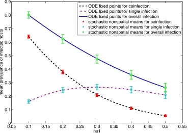
0.050 0.1 0.15 0.2 0.25 0.3 0.35 0.4 0.45 0.5 0.55 0.1

0.2 0.3 0.4 0.5 0.6 0.7 0.8 0.9

nu1

mean prevalence of infected hosts

ODE fixed points for coinfection ODE fixed points for single infection ODE fixed points for overall infection stochastic nonspatial means for coinfection stochastic nonspatial means for single infection stochastic nonspatial means for overall infection

To compare the fixed points and stochastic model means, I start by finding the

fixed points for the baseline model parameters. When the fixed points of the baseline

model are added together, we can see that the overall prevalence of infection

((IA+IB+IX)/N) decreases as the death rate,

€

ν1, increases (Fig. 3). Similarly, the fixed point

for the prevalence of coinfected hosts (IX/N) decreases as the death rate increases.

However, when the slopes of the coinfection and overall infection lines are compared, the

rate at which coinfection decreases is different from the rate at which the overall

(34)

prevalence of infection decreases (Fig. 3). For 0.1 <

€

ν1 < 0.3, there is a greater decrease

in the prevalence of coinfection than in the prevalence of overall infection. With the

number of coinfected hosts decreasing more than overall infected hosts, the prevalence of

singly infected hosts ((IA+IB)/N) must increase so that the number of coinfected hosts plus

the number of singly infected hosts equals the overall number of infected hosts (Fig. 3).

However, for 0.3 <

€

ν1_{< 0.5, overall prevalence of infection decreases more than the}

prevalence of coinfection. As the difference between coinfection and overall infection

decreases, the fixed point for the prevalence of singly infected hosts also must decrease.

To compare the ODE model to the stochastic nonspatial model, we overlay the

mean prevalence of infection from the stochastic nonspatial model on the fixed points

from the deterministic ODE model (Fig. 3). For coinfection, single infection, and overall

infection, the comparison shows that the fixed points and the mean prevalence of

infection are approximately equal. The fixed points from the ODE model and the means

from the stochastic nonspatial model are also approximately equal in all the model

variations.

2. Baseline Model

The baseline model simulates a system in which there is no interaction between

the two pathogens. We explore the simulations under this scenario to compare the mean

(35)

examine the neighboring probabilities of infection (eqs. 1-4) to determine if aggregation

is responsible for the difference in prevalence of infection between the two models.

2.1 Stochastic Nonspatial Model

Results from the stochastic nonspatial model parallel the results from the

nonspatial ODE model, but are provided again here for comparison with the stochastic

spatial model. Simulations of the baseline model were run for

€

ν1 = 0.1, 0.2, 0.3, 0.4, and

0.5. The baseline simulations result in a decrease in coinfection as the death rate

increases (Fig. 4a). For small values of

€

ν1, the prevalence of singly infected hosts

increases while the prevalence of coinfected hosts decreases. However, when the

infection-induced death rate becomes larger, both the prevalence of coinfected hosts and

the prevalence of singly infected hosts decrease (Fig. 4). The overall prevalence of

infection also decreases as the death rate increases.

2.2 Stochastic Spatial Model

The stochastic spatial model simulations result in similar trends to the stochastic

nonspatial model. As

€

ν1 increases, the prevalence of coinfected hosts decreases in both

models (Fig. 4a). Similar to the nonspatial model, the spatial model also shows an

increase in the prevalence of singly infected hosts followed by a decrease as the death

(36)

0.050 0.1 0.15 0.2 0.25 0.3 0.35 0.4 0.45 0.5 0.55 0.1 0.2 0.3 0.4 0.5 0.6 0.7 0.8 0.9 nu1

mean prevalence of infecteds

nonspatial spatial n=4 spatial n=8

0.050 0.1 0.15 0.2 0.25 0.3 0.35 0.4 0.45 0.5 0.55 0.05 0.1 0.15 0.2 0.25 0.3 0.35 0.4 nu1

0.050 0.1 0.15 0.2 0.25 0.3 0.35 0.4 0.45 0.5 0.55

0.1 0.2 0.3 0.4 0.5 0.6 0.7 nu1

nonspatial spatial n=4 spatial n=8 a) b) c)

Figure 4. The mean prevalence of infection for the baseline model. Symbols represent mean prevalence of infected hosts. Vertical lines represent standard deviations. Dashed line is spatial n=4 model. Solid line is spatial n=8 model. Dashed-dotted line is

(37)

Although similar in some respects, the spatial and nonspatial models result in

some differences too. The effect of spatial structure on the mean prevalence of singly

infected hosts depends on the value of the infection death rate. For small values of

€

ν1,

the mean prevalence of singly infected hosts increases with localized transmission (Fig.

4b). This result may be a product of aggregation, which we explore through the

neighboring probabilities of infection (eqs. 1-4). However, for larger values of

€

ν1, the

mean prevalence of singly infected hosts decreases with localized transmission. Some of

this behavior can be explained by looking at the overall prevalence of infection (Fig. 4c).

At low values of the death rate, overall infection is similar for both the nonspatial and

spatial model so aggregation appears to explain the increase in singly infected hosts with

localization. However, as the death rate increases, overall infection decreases more

rapidly with localization, causing the prevalence of singly infected hosts to also decrease

with localization.

As transmission becomes more localized, the mean number of coinfected hosts

decreases for all the infection death rates analyzed (Fig. 4a). This result also reflects the

decrease in overall infection as transmission becomes more localized. Both the decrease

in coinfected hosts and the decrease in overall infection with increased localization are

similar to results from a one-pathogen model, where localization decreases overall

prevalence of infection (Keeling 1999). In the one-pathogen model, the decrease is due

to a limited number of susceptible contacts (Tildesley et al. 2010, Brown and Bolker

(38)

between hosts infected by different pathogens becomes limited with localization,

especially if aggregation occurs.

To determine the mechanism causing the decrease in coinfected hosts with

increased localization, we examine the neighboring probabilities of infection (eqs. 1-4).

By comparing P(A|A) to P(B|A), we can determine if hosts infected by pathogen A are

spatially aggregated. Pathogen A and pathogen B are indistinguishable, so the results of

the neighboring probabilities of infection for pathogen A can also be extended to

pathogen B. Probabilities from the simulations run for

€

ν1 = 0.5 are not included, because

no infected individuals remained by the end of the simulation for the spatial n=4 model.

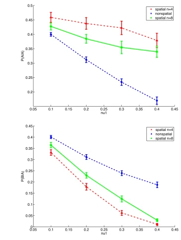
In the nonspatial model, the conditional probabilities P(A|A) and P(B|A) are

approximately the same, meaning that hosts with pathogen A are as likely to be next to a

host with pathogen A as to be next to a host with pathogen B (Fig. 5). This occurs

because in the nonspatial model the neighboring probabilities of infection depend on the

total number of infected individuals in the population. With the total number of hosts

infected by pathogen A and pathogen B being approximately equal in the nonspatial

model, the probabilities P(A|A) and P(B|A) are approximately equal. This makes it easy

to determine the differences between P(A|A) and P(B|A) in the spatial model.

Comparing P(A|A) to P(B|A) in the spatial model shows that a host infected with

pathogen A is more likely to be next to another host infected by pathogen A than next to

a host infected by pathogen B. Because P(A|A) is greater than P(B|A), these probabilities

(39)

0.05 0.1 0.15 0.2 0.25 0.3 0.35 0.4 0.45 0.2

0.25 0.3 0.35 0.4 0.45 0.5

nu1

P(A|A)

spatial n=4 nonspatial spatial n=8

0.050 0.1 0.15 0.2 0.25 0.3 0.35 0.4 0.45 0.05

0.1 0.15 0.2 0.25 0.3 0.35 0.4 0.45

nu1

P(B|A)

spatial n=4 nonspatial spatial n=8 a)

b)

Figure 5. Aggregation of pathogen A. Symbols represent the mean prevalence of

infecteds. Vertical lines represent standard deviations. The dashed line is the nonspatial model. The solid line is the spatial n=8 model. The dashed-dotted line is the spatial n=4 model. (a) The probability of a host infected by pathogen A neighboring another host infected by pathogen A. (b) The probability of a host infected by pathogen A

(40)

5 10 15 20 25 30 35 40 45 50

and P(B|A) increases with increased localization, indicating that spatial aggregation of

pathogen A increases with localization (Fig. 5). The same results occur for the

probabilities for pathogen B indicating that hosts infected by pathogen B are also

spatially aggregated. These results indicate that spatial aggregation is keeping the two

pathogens separated, providing a possible explanation for why there is less coinfection in

the spatial model. The separation becomes apparent when examining a map of the lattice,

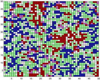
where we can see clumps of pathogen A and clumps of pathogen B (Fig. 6). Coinfected

Figure 6. Map of the lattice to show aggregation in the baseline model. Taken from the spatial n=4 model. Time=250, ν1=0.3. White represents vacant patches. Green

(41)

hosts can be included with either pathogen A or pathogen B to extend the clumps further.

The clumps of pathogen A and the clumps of pathogen B are usually separated by

susceptible hosts and vacant patches, creating spatial segregation.

Why does aggregation lead to a decrease in coinfection and an increase in single

infection? Aggregation causes a host infected only by pathogen A to be surrounded by

other hosts infected only by pathogen A. This means that the host has no neighbors with

pathogen B, so the host cannot become infected by pathogen B. A similar argument

holds for a host with pathogen B. Thus aggregation leads to a decrease in the number of

coinfected hosts and an increase in the number of singly infected hosts. Aggregation in

the spatial model provides a reason for why we see a decrease in coinfection and an

increase in single infection.

3. Cross-Protection

In a system with cross-protection, one pathogen prevents a second pathogen from

infecting the host. Consequently, the rate at which hosts become coinfected is reduced.

To demonstrate cross-protection in this set of simulations, we set k = 0.5 to reduce the rate of coinfection.

In the cross-protection model, the overall prevalence of infection is approximately

the same as in the baseline model (compare Fig. 4c & Fig. 7c). However, the

(42)

0.050 0.1 0.15 0.2 0.25 0.3 0.35 0.4 0.45 0.5 0.55 0.1 0.2 0.3 0.4 0.5 0.6 0.7 0.8 0.9 nu1

mean prevalence of infected hosts

0.050 0.1 0.15 0.2 0.25 0.3 0.35 0.4 0.45 0.5 0.55 0.05 0.1 0.15 0.2 0.25 0.3 0.35 0.4 0.45 0.5 nu1

0.050 0.1 0.15 0.2 0.25 0.3 0.35 0.4 0.45 0.5 0.55 0.1 0.2 0.3 0.4 0.5 0.6 nu1

(43)

the value of

€

ν1, because of the slowed rate at which hosts transition from single infection

to coinfection in the cross-protection model (compare Fig. 4a & Fig. 7a). In order to

keep the overall infection prevalence the same in both the cross-protection model and the

baseline model, the prevalence of singly infected hosts must compensate for the decrease

in coinfected hosts. Therefore, the cross-protection model results in an increase in the

prevalence of singly infected hosts compared to the baseline model for each

€

ν1 analyzed

(compare Fig. 4b & Fig. 7b). This result shows that as the rate at which hosts gain a

second pathogen decreases, the prevalence of coinfected hosts also decreases. The case

when this rate is zero, or in terms of the model when k=0, is a limiting case that helps build intuition. In this case, hosts do not become coinfected so we would expect only

singly infected hosts to remain.

Similar to the nonspatial model, the spatial cross-protection model results in

approximately the same overall prevalence of infection as in the spatial baseline model,

but with a decrease in coinfection and an increase in single infection (compare Fig. 4 &

Fig. 7). In addition to being the result of a lower coinfection rate, the decrease in

coinfected hosts and increase in singly infected hosts is the result of a difference in

aggregation between the spatial models. The cross-protection model produces a small

increase in aggregation compared to the baseline model. The probability of a host

infected by pathogen A having a neighbor also infected by pathogen A increases by 0.025

(44)

by pathogen B decreases by 0.02 to 0.047 in the cross-protection model, except for when

€

ν1 = 0.4 where the difference is almost equal to 0.

Similar to the baseline model, the cross-protection model maintains the same

relationship between the spatial and nonspatial model. The mean number of coinfected

hosts decreases with increased localization (Fig. 7a). At the same time, the mean number

of singly infected hosts increases with increased localization for small values of

€

ν1 and

decreases with localization for large values of

€

ν1 (Fig. 7b). This relationship between the

spatial and nonspatial models remains the same for all variations unless otherwise stated.

4. Synergism – Increased Transmission

One effect that occurs when two pathogens interact within the same organism is

an increased pathogen transmission rate. To represent increased transmission rates due to

synergism, we set k=5 to increase the rate at which a singly infected host becomes doubly infected.

Again, the overall prevalence of infection is the same in the increased

transmission model as in the baseline model. However, hosts are becoming coinfected at

a faster rate in the increased transmission model than in the baseline model, so the

prevalence of coinfected hosts increases in the increased transmission model (compare

Fig. 4a & Fig. 8a). While the rate at which singly infected hosts become coinfected

(45)

0.050 0.1 0.15 0.2 0.25 0.3 0.35 0.4 0.45 0.5 0.55 0.1 0.2 0.3 0.4 0.5 0.6 0.7 0.8 0.9 nu1

nonspatial spatial n=4 spatial n=8 0.050 0.1 0.15 0.2 0.25 0.3 0.35 0.4 0.45 0.5 0.55 0.1 0.2 0.3 0.4 0.5 0.6 nu1

0.050 0.1 0.15 0.2 0.25 0.3 0.35 0.4 0.45 0.5 0.55 0.02 0.04 0.06 0.08 0.1 0.12 0.14 0.16 nu1

(46)

decrease in the prevalence of singly infected hosts (compare Fig. 4b & Fig. 8b). The

increase in coinfection and similar decrease in single infection allows the overall

prevalence of infection in the increased transmission model to remain approximately

equal to the overall prevalence of infection in the baseline model (compare Fig. 4c & Fig.

8c).

The spatial model with increased transmission results in a decrease in aggregation

compared to the baseline model. This decreased aggregation is shown through a decrease

in P(A|A) of 0.032-0.11 and an increase in P(B|A) of 0.016-0.071, depending on the

value of

€

ν1 and the degree of localization. The decreased aggregation means that the two

pathogens are not as spatially separated in the increased transmission model. With less

pathogen separation, the two pathogens are more likely to come into contact with each

other. Therefore, the increased transmission model results in an increase in the

prevalence of coinfected hosts compared to the baseline model. However, the overall

prevalence of infection is approximately the same in both the increased transmission

model and the baseline model, so the increase in coinfected hosts is reflected by a

(47)

5. Synergism – Increased Mortality

A second effect of pathogen interaction within a host is increased host mortality.

To represent increased mortality due to synergism, we set

€

ν2=ν1 to increase the rate at

which coinfected hosts die.

With

€

ν2 =ν1, the death rate for coinfected hosts is double the death rate for singly

infected hosts. This means that when

€

ν1=ν2 =0.25 the death rate for coinfected hosts is

0.5, which is the highest death rate we examined under the other scenarios. In addition,

the rate at which singly infected hosts become coinfected remains unchanged from the

baseline model, but coinfected hosts die faster. This produces a large decrease in the

prevalence of coinfected hosts in the increased mortality model compared to the baseline

model (compare Fig. 4a & Fig. 9a). The overall prevalence of infection also decreases in

the increased mortality model, but not as much as coinfection decreases (compare Fig. 4c

& Fig. 9c). Reflecting the difference between coinfection and overall infection, the

prevalence of singly infected hosts increases in the increased mortality model compared

to the baseline model (compare Fig. 4b & Fig. 9b).

For these simulations, we are only able to draw conclusions from

€

ν1,ν2∈[0.05,0.25], because larger values of

€

ν2 cause one of the pathogens to become

(48)

0 0.05 0.1 0.15 0.2 0.25 0.3 0.35

0.2 0.3 0.4 0.5 0.6 0.7 0.8 nu1

0 0.05 0.1 0.15 0.2 0.25 0.3 0.35

0 0.1 0.2 0.3 0.4 0.5 0.6 0.7 nu1

0 0.05 0.1 0.15 0.2 0.25 0.3 0.35 0.1 0.15 0.2 0.25 0.3 0.35 0.4 0.45 0.5 0.55 0.6 nu1

(49)

informative, because the number of infected hosts does not oscillate around an

equilibrium point. Rather the number of infected hosts decreases until there are no more

infected hosts. This result produces a very large standard deviation, making the mean

unreliable for large values of

€

ν2. Instead, we explore the cases where

€

ν2 > 0.25 by

looking at extinction probabilities in section 5.3.

Similar to the nonspatial model, the spatial model with increased mortality results

in a decrease in the prevalence of coinfected hosts and an increase in the prevalence of

singly infected hosts compared to the baseline model. The rapid decrease in coinfection

in the spatial model can be explained through aggregation. With increased mortality, the

P(A|A) increases as the death rate increases unlike in the baseline model where P(A|A)

decreases as the death rate increases (compare Fig. 5a & Fig. 10a). In addition, P(B|A)

exhibits a large decrease in the increased mortality model compared to the baseline

model, almost reaching zero by the time the death rate is 0.2 (compare Fig. 5b & Fig.

10b). Considering these conditional probabilities and comparing them to the baseline

model, the increased mortality model indicates a large amount of aggregation of pathogen

A especially at larger death rates. With the pathogens being indistinguishable, we see

(50)

0.04 0.06 0.08 0.1 0.12 0.14 0.16 0.18 0.2 0.22 0.2

0.25 0.3 0.35 0.4 0.45 0.5 0.55 0.6 0.65

nu1

P(A|A)

0.040 0.06 0.08 0.1 0.12 0.14 0.16 0.18 0.2 0.22

0.05 0.1 0.15 0.2 0.25 0.3 0.35 0.4 0.45

nu1

P(B|A)

a)

b)

Figure 10. Aggregation of pathogen A in the increased mortality model. Symbols

(51)

5.3 Extinction Probability

The simulations for the nonspatial model with increased mortality resulted in

extinction of one pathogen for the larger values of

€

ν1. Because of this result, we decided

to study the extinction times for the increased mortality scenario. To determine

extinction times, we ran 100 simulations of each model for a maximum time of 500 under

both

€

ν2 =ν1=0.3 and

€

ν2=ν1=0.4. The results of these simulations are studied by

comparing the probability of extinction for the nonspatial model to the spatial model.

The results of these simulations show that extinction occurs faster and more often

in the nonspatial model compared to the spatial model. For both death rates, all 100 of

the nonspatial model simulations reached extinction before reaching the maximum time

of 500 (Fig. 11). Only a few of the spatial model simulations reached extinction by time

500. Specifically, only one simulation for a neighborhood size of four and only six

simulations for a neighborhood size of eight reached extinction before time 500 when

€

ν2 =ν1=0.3 (Fig. 11a). For

€

ν2=ν1=0.4, only five simulations for a neighborhood size

of four and only nine simulations for a neighborhood size of eight reached extinction

before time 500 (Figure 11b). To understand the extinction behavior better, we can look

at the average time to extinction. For the nonspatial model, the average time to extinction

is 206.2 for

€

ν2 =ν1=0.3 and 118.0 for

€

ν2=ν1=0.4. On the other hand, the average

(52)

0 50 100 150 200 250 300 350 400 450 500

0 10 20 30 40 50 60 70 80 90 100 time

frequency of extinction of one pathogen

0 50 100 150 200 250 300 350 400 450 500

0 10 20 30 40 50 60 70 80 90 100 time

frequency of extinction of one pathogen

a)

b)

Figure 11. Time of extinction of one pathogen. The dashed line is the spatial n=4 model. The solid line is the spatial n=8 model. The dashed-dotted line is the nonspatial model. (a) Time of extinction of one pathogen for

€

ν2=ν1=0.3. (b) Time of extinction of one

pathogen for

€

(53)

These results imply that the probability of extinction of one pathogen increases as

localization decreases. One reason that localization increases the probability that both

pathogens persist may be that localization produces aggregation as can be seen through

the conditional probabilities for the spatial model. In the spatial n=4 model where

€

ν2 =ν1=0.3, P(A|A) is 0.4645 and P(B|A) is 0.0164. In the spatial n=4 model where

€

ν2=ν1=0.4, P(A|A) is 0.3854 and P(B|A) is 0.0028. Although these numbers are taken

from one simulation, these conditional probabilities give approximately the same values

as all other simulations run. For both death rates, the neighboring probabilities of

infection indicate that a host with pathogen A is much more likely to be next to another

host with pathogen A than next to a host with pathogen B. This large degree of

aggregation is due to coinfected hosts dying quickly and being replaced by vacant

patches. The vacant patches provide spatial separation of hosts infected by A and hosts

infected by B. With this large amount of spatial separation through aggregation, contact

between the two pathogens is limited in the spatial model, making it more difficult for

one pathogen to outcompete the other pathogen. Therefore, both pathogens are able to

(54)

Discussion

1. Conclusions and Biological Implications

Mathematical models are useful, noninvasive tools for making predictions about

disease dynamics, which can then be tested in the field. However, most of the current

models assume a “well-mixed” population (Bailey 1975; Boylan 1991; Brauer 2008;

Brown and Bolker 2004; Lefevre 1983). This assumption is unrealistic in many cases,

especially for plant communities where the hosts are incapable of moving to interact with

other hosts (Brown and Bolker 2004). In this case, spatial structure must be taken into

consideration to explore the spread of infection. Some one-pathogen models incorporate

spatial structure, providing a good foundation, but often multiple pathogens are capable

of inhabiting a single organism requiring a more complicated model (Seabloom 2009).

The addition of both multiple pathogens and spatial structure to a host-pathogen model

raises some new questions. How does spatial structure affect the prevalence of single

infection and coinfection? Is pathogen clustering responsible for the changes in

infection? How do within-host interactions among pathogens (e.g. cross-protection and

synergism) affect the prevalence of single infection and coinfection? With the use of the

two-pathogen model presented here, we can begin to answer these questions.

Through examining and comparing two-pathogen nonspatial and spatial models,

we learn that the dynamics of coinfection depend on the infection-induced death rate and

the degree of localization. When pathogens do not interact directly, increasing the

Spatial Dnamics of Infection by Multiple Pathogens: A Case Study with Yellow Dwarf Virus.

Abstract

Biography

Acknowledgements

Table of Contents

List of Tables

List of Figures

Introduction

1. Overview

2. Mathematical Tools for Analyzing Nonspatial and Spatial Models

3. Spatial Structure in One-Pathogen Models

4. Two-Pathogen Models

Methods

1. Models and Their Architecture

2. Biological Scenarios and Parameter Values

3. Simulation Details for Stochastic Models

∑

∑

Results

1. Nonspatial Models

2. Baseline Model

3. Cross-Protection

4. Synergism – Increased Transmission

5. Synergism – Increased Mortality

Discussion

1. Conclusions and Biological Implications