BOAGGIO, KATIE LISA. Storm Track Sensitivity to Resolution and Climate Change in High-Resolution Global Simulations (Under the direction of Dr. Walter A. Robinson).
Simulations
by
Katie Lisa Boaggio
A thesis submitted to the Graduate Faculty of North Carolina State University
in partial fulfillment of the requirements for the degree of
Master of Science
Marine, Earth, and Atmospheric Sciences
Raleigh, North Carolina 2019
APPROVED BY:
______________________________ _______________________________ Dr. Gary M. Lackmann Dr. Anantha Aiyyer
_______________________________ Dr. Walter A. Robinson
BIOGRAPHY
I am originally from a town in South Jersey called Voorhees right outside of
ACKNOWLEDGMENTS
I would like to thank my advisor, Dr. Walt Robinson, for his constant support and help throughout this entire process. He made sure to help me break down every single problem I had, whether it be a coding issue or a conceptual problem, and made sure I understood what to do. I would also like to thank Dr. Gary Lackmann and Dr. Anantha Aiyyer for helping me think of other factors and variables to investigate throughout the later portion of my project. I am grateful to have had the opportunity to work with such a knowledgeable and encouraging committee. I would also like to extend a thank you to Allison Michaelis for providing me with the MPAS data and assisting me with understanding the structure and format of the data. Finally, I’d like to
thank my friends and fellow graduate students for their constant support, love, and confidence in me throughout this entire process. I would not have made it to this point without their
TABLE OF CONTENTS
LIST OF TABLES ... v
LIST OF FIGURES ... vi
1. Introduction ... 1
1.1. Motivation ... 1
1.2. Literature review ... 3
1.2.1. Storm tracks ... 3
1.2.2. Climate warming projections ... 4
1.2.3. Horizontal resolution... 6
2. Data and Methods ... 8
2.1. Model descriptions ... 8
2.1.1. UPSCALE ... 8
2.1.2. MPAS ... 9
2.2. Storm track analysis ... 11
2.2.1. Local deepening rate (LDR) ... 11
2.2.2. Other metrics ... 11
2.3. Case study analysis ... 14
3. Results I: Effects of Resolution ... 17
3.1. Multi-model analysis ... 17
3.1.1. Resolution results ... 17
3.1.2. Atlantic storm track analysis ... 19
3.1.3. Pacific storm track analysis.. ... 22
3.2. A strong case study... 23
3.2.1. UPSCALE low-resolution storm ... 24
3.2.2. UPSCALE high-resolution storm ... 24
3.2.3. Discussion of differences ... 25
4. Results II: Effects of Climate Warming ... 50
4.1. UPSCALE model analysis ... 50
4.1.1. Future changes ... 50
4.1.2. Atlantic storm track analysis ... 51
4.1.3. Pacific storm track analysis.. ... 53
4.2. MPAS model analysis ... 56
4.2.1. Future changes ... 56
4.2.2. Atlantic storm track analysis ... 57
4.2.3. Pacific storm track analysis.. ... 58
4.3. Model differences.. ... 60
5. Summary and Conclusions ... 103
LIST OF TABLES
LIST OF FIGURES
Figure 2.1: The 26-year average difference between future and current sea surface
temperature (SSTs) anomalies in the UPSCALE 25km simulations. ... 15 Figure 2.2: The 10-year average difference between future and current sea surface
temperature (SSTs) anomalies in the MPAS 15km simulations. ... 16 Figure 3.1: The average wintertime (DJF) local deepening rate (LDR), measured in
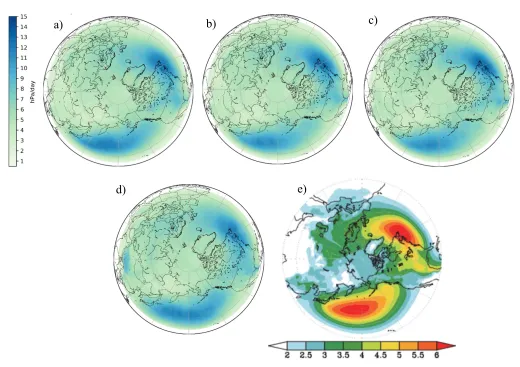
hPa/day, over the 26-year period from 1985-2011 for a) UPSCALE 130km, b) UPSCALE 60km, c) UPSCALE 25km, over the 10-year period for c) MPAS 15km, and d) the climatological mean wintertime (DJF) LDR between 1958 and 2013 (Kuwano-Yoshida 2014). For a)-d), the domain is the Northern
hemisphere and the values were set to zero past 20⁰N. ... 27
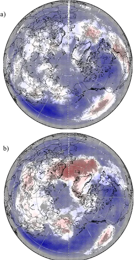
Figure 3.2: The climate warming differences (future minus current) of the average
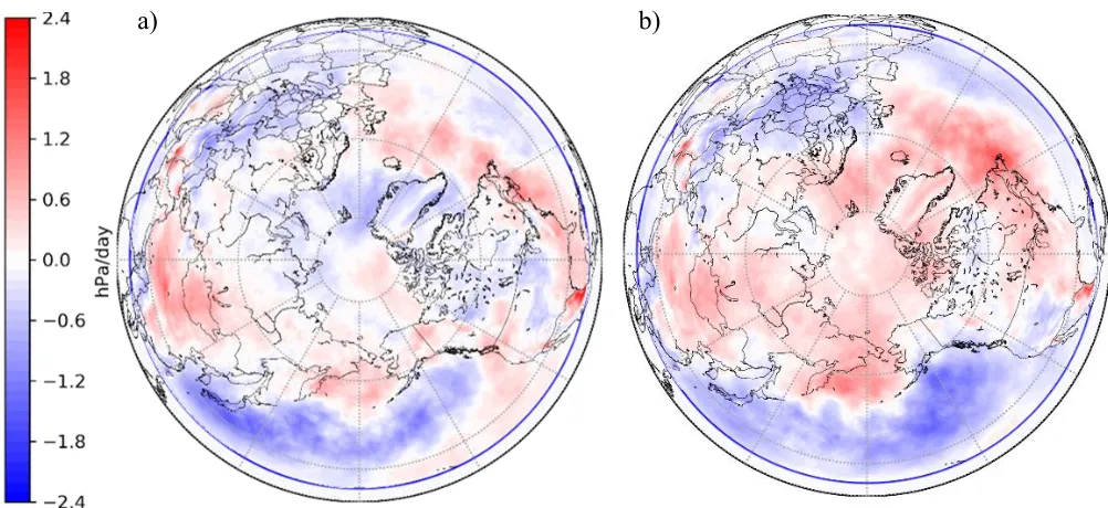
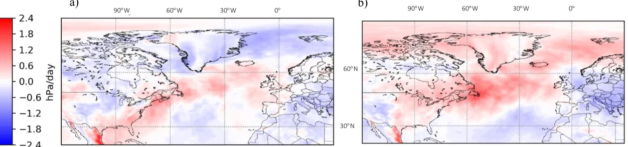
wintertime LDR, measured in hPa/day, for UPSCALE a) 130km and b) 25km is shaded below circular hatching that shows where all ensemble members (5 for 130km, 3 for 25km) agree on the sign of the change. ... 28 Figure 3.3: The resolution differences, higher (25km) minus lower (130km), of the average
wintertime LDR for a) present and b) future UPSCALE simulations, with units hPa/day. The domain is the Northern hemisphere and the values were set to zero past 20⁰N. ... 29
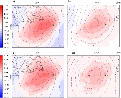
Figure 3.4: The precipitation rate covariance with the local deepening rate for UPSCALE present a) 130km in the West Atlantic, b) 130km in the East Atlantic, c) 25km in the West Atlantic, and d) 25km in the East Atlantic. The base point (green star) is at 45 N, 45 W in the West Atlantic and 50 N, 20 W in the East Atlantic and units are in mm/day. The contours are the mean sea level pressure covariance with the local deepening rate for each respective simulation. The
units are mb. ... 30
Figure 3.5: The resolution differences, higher (25km) minus lower (130km), of the average wintertime LDR for a) present and b) future UPSCALE simulations, with units hPa/day in the Atlantic basin. ... 31
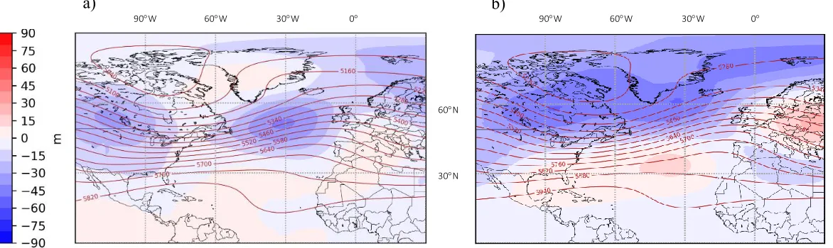
Figure 3.6: The resolution differences, higher (25km) minus lower (130km), of the average wintertime 500-hPa geopotential heights are shaded for a) present and b) future UPSCALE simulations in the Atlantic basin with units of meters (m). The contours show the high resolution, present geopotential heights with units of
Pascals (Pa) in a) and the high resolution, future geopotential heights in b). ... 32
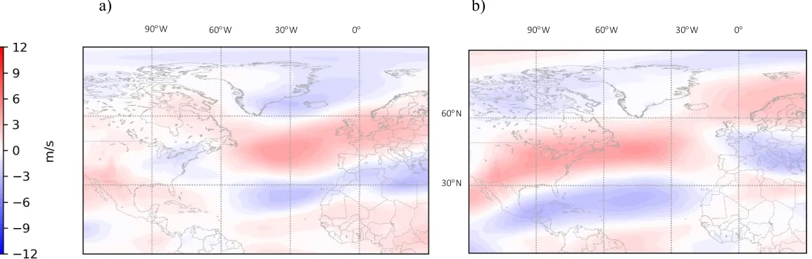
Figure 3.8: The resolution differences, higher (25km) minus lower (130km), of the lower level (850hPa) zonal winds for a) present and b) future UPSCALE simulations in the Atlantic basin with units of m/s. ... 34
Figure 3.9: The resolution differences, higher (25km) minus lower (130km), of the Eady growth rate for a) present and b) future UPSCALE simulations in the Atlantic basin with units of day-1. ... 35
Figure 3.10: The resolution differences, higher (25km) minus lower (130km), of the average wintertime LDR for a) present and b) future UPSCALE simulations, with units hPa/day in the Pacific basin. ... 36
Figure 3.11: The resolution differences, higher (25km) minus lower (130km), of the average wintertime 500-hPa geopotential heights are shaded for a) present and b) future UPSCALE simulations in the Pacific basin with units of meters (m). The contours show the high resolution, present geopotential heights with units of
Pascals (Pa) in a) and the high resolution, future geopotential heights in b). ... 37
Figure 3.12: The resolution differences, higher (25km) minus lower (130km), of the upper level (500hPa) zonal winds for a) present and b) future UPSCALE simulations in the Pacific basin with units of m/s. ... 38
Figure 3.13: The resolution differences, higher (25km) minus lower (130km), of the lower level (850hPa) zonal winds for a) present and b) future UPSCALE simulations in the Pacific basin with units of m/s. ... 39
Figure 3.14: The resolution differences, higher (25km) minus lower (130km), of the Eady growth rate for UPSCALE a) present and b) future Pacific with units of day-1. ... 40
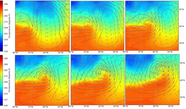
Figure 3.15: The strong case from the UPSCALE present-day 130km simulations. The temperature (K) is shown in color shading, the mean sea level pressure (hPa) is contoured on top in red, and surface wind barbs are shown in grey. This shows the peak of the strong storm, which occurred around December 7th-10th, 1990 in one of the 130km ensemble members. The time between panels is 6 hours and the largest drop in pressure (largest LDR value) occurred between 12Z on 12/8 and 12Z on 12/9 (2nd and 3rd panels).. ... 41
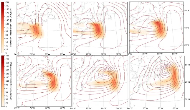
Figure 3.16: The strong storm case from the UPSCALE present-day 130km simulations. The precipitation rate (mm/day) is shown in color shading, while the mean sea level pressure (hPa) is contoured on top in red. This shows the peak of the strong storm, which occurred around December 7th-10th, 1990 in one of the 130km
ensemble members. The time between panels is 6 hours and the largest drop in pressure (largest LDR value) occurred between 12Z on 12/8 and 12Z on 12/9
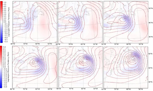
Figure 3.17: The strong case from the UPSCALE present-day 130km simulations. The pressure vertical velocity (-Pa/s) is shown in color shading, while the mean sea level pressure (hPa) is contoured on top in red. This shows the peak of the strong storm, which occurred around December 7th-10th, 1990 in one of the
130km ensemble members. The time between panels is 6 hours and the largest drop in pressure (largest LDR value) occurred between 12Z on 12/8 and 12Z
on 12/9 (2nd and 3rd panels). ... 43 Figure 3.18: The strong storm case from the UPSCALE present-day 25km simulations. The
temperature (K) is shown in color shading, the mean sea level pressure (hPa) is contoured on top in red, and surface wind barbs are shown in grey. This shows the peak of the strong storm, which occurred around February 18th-21st, 1995 in one of the 25km ensemble members. The time between panels is 6 hours and the largest drop in pressure (largest LDR value) occurred between 12Z on 2/19 and 12Z on 2/20 (4th and 5th panels). ... 44
Figure 3.19: The strong storm case from the UPSCALE present-day 25km simulations. The precipitation rate (mm/day) is shown in color contours while the mean sea level pressure (hPa) is contoured on top in red. This shows the peak of the strong storm, which occurred around February 18th-21st, 1995 in one of the 25km ensemble members. The time between panels is 6 hours and the largest drop in pressure (largest LDR value) occurred between 12Z on 2/19 and 12Z on 2/20
(4th and 5th panels). ... 45 Figure 3.20: The strong storm case from the UPSCALE present-day 25km simulations.
The pressure vertical velocity (Pa/s) is shown in color contours while the mean sea level pressure (hPa) is contoured on top in red. This shows the peak of the strong storm, which occurred around February 18th-21st, 1995 in one of the
25km ensemble members. The time between panels is 6 hours and the largest drop in pressure (largest LDR value) occurred between 12Z on 2/19 and 12Z
on 2/20 (4th and 5th panels)... 46
Figure 3.21: Across the transect shown in a), the vertical cross section of the atmospheric temperature is shown in b) for the peak of the strong storm at 130km in the
UPSCALE simulations ... 47 Figure 3.22: Across the transect shown in a), the vertical cross section of the atmospheric
temperature is shown in b) for the peak of the strong storm at 25km in the
UPSCALE simulations. ... 48 Figure 3.23: Across the transects shown in a) at 130km UPSCALE and b) at 25km
Figure 4.1: The average wintertime (DJF) local deepening rate (LDR), measured in
hPa/day, over the 26-year future end of century period for a) UPSCALE 130km, b) UPSCALE 60km, c) UPSCALE 25km. The domain is the Northern
hemisphere and the values were set to zero past 20⁰N. ... 63
Figure 4.2: The climate warming differences, future minus present, of the average wintertime LDR for a) UPSCALE 130km, b) UPSCALE 60km and c)
UPSCALE 25km simulations. The domain is the Northern hemisphere and the values were set to zero past 20⁰N. ... 64
Figure 4.3: The climate warming differences, future minus present, of the precipitation rate covariance with the local deepening rate for UPSCALE 25km a) West Atlantic, b) and East Atlantic. The base point (green star) is at 45 N, 45 W in the West Atlantic and 50 N, 20 W in the East Atlantic and units are in mm/day. The contours are the climate warming differences of the mean sea level pressure covariance with the local deepening rate for each respective simulation. The
units are mb. ... 65
Figure 4.4: The climate warming differences, future minus present, of the average wintertime LDR for a) UPSCALE 130km and b) UPSCALE 25km in the Atlantic basin.
... 66 Figure 4.5: The climate warming differences, future minus present, of the average
wintertime 500-hPa geopotential heights shaded for a) 130km and b) 25km UPSCALE simulations in the Atlantic basin with units of meters (m). The contours show the low resolution, present geopotential heights with units of
Pascals (Pa) in a) and the high resolution present geopotential heights in b). ... 67
Figure 4.6: The climate warming differences, future minus present, of the upper level (300hPa) zonal winds for a) 130km and b) 25km UPSCALE simulations in the Atlantic basin with units of m/s. ... 68
Figure 4.7: The climate warming differences, future minus present, of the lower level (850hPa) zonal winds for a) 130km and b) 25km UPSCALE simulations in the Atlantic basin with units of m/s. ... 69
Figure 4.8: The climate warming differences, future minus present, of the Eady growth rate for UPSCALE a) 130km and b) 25km Atlantic with units of day-1. ... 70
Figure 4.9: The climate warming differences, future minus present, of the precipitation rate covariance with the local deepening rate for UPSCALE a) 130km and b) 25km in the East Pacific. The base point (green star) is at 45 N, 150 W in the East Pacific and units are in mm/day. The contours are the climate warming
Figure 4.10: The climate warming differences, future minus present, of the average wintertime LDR for a) UPSCALE 130km and b) UPSCALE 25km in the
Atlantic basin. ... 72
Figure 4.11: The climate warming differences, future minus present, of the average wintertime 500-hPa geopotential heights shaded for a) 130km and b) 25km UPSCALE simulations in the Pacific basin with units of meters (m). The contours show the low resolution, present geopotential heights with units of
Pascals (Pa) in a) and the high resolution present geopotential heights in b). ... 73
Figure 4.12: The climate warming differences, future minus present, of the upper level (300hPa) zonal winds for a) 130km and b) 25km UPSCALE simulations in the Pacific basin with units of m/s. The dotted black line indicates the present-day Jetstream axis. ... 74
Figure 4.13: The climate warming differences, future minus present, of the lower level (850hPa) zonal winds for a) 130km and b) 25km UPSCALE simulations in the Pacific basin with units of m/s. ... 75
Figure 4.14: The climate warming differences, future minus present, of the Eady growth rate for UPSCALE a) 130km and b) 25km Pacific with units of day-1. ... 76
Figure 4.15: A time series of the Niño 3.4 average wintertime SST with the global mean SST subtracted off. The blue line is the UPSCALE 25km present-day SST and the red line is the UPSCALE 25km future SST. ... 77
Figure 4.16: The difference between the LDR from the five strongest El Niño years minus the five strongest La Niña years for UPSCALE a) 130km and b) 25km. The
units are hPa/day. ... 78
Figure 4.17: The average wintertime (DJF) local deepening rate (LDR), measured in hPa/day, over the 10-year future end of century period for the MPAS 15km simulations. The domain is the Northern hemisphere and the values were set to zero past 20⁰N. ... 79
Figure 4.18: The climate warming differences, future minus present, of the average
wintertime LDR for the MPAS 15km simulations. The domain is the Northern
hemisphere and the values were set to zero past 20⁰N. ... 80
Figure 4.19: The precipitation rate covariance with the local deepening rate for MPAS present 15km in the a) West Atlantic and b) East Atlantic. The base point (green star) is at 45 N, 45 W in the West Atlantic and 50 N, 20 W in the East Atlantic and units are in mm/day. The contours are the mean sea level pressure covariance with the local deepening rate for each respective simulation. The
Figure 4.20: The climate warming differences, future minus present, of the precipitation rate covariance with the local deepening rate for MPAS 15km a) West Atlantic, b) and East Atlantic. The base point (green star) is at 45 N, 45 W in the West
Atlantic and 50 N, 20 W in the East Atlantic and units are in mm/day. ... 82
Figure 4.21: The climate warming differences, future minus present, of the average
wintertime LDR for MPAS 15km in the Atlantic basin. ... 83
Figure 4.22: The climate warming differences, future minus present, of the average
wintertime 500-hPa geopotential heights shaded for 15km MPAS simulations in the Atlantic basin with units of meters (m). The contours show the present
geopotential heights with units of Pascals (Pa). ... 84
Figure 4.23: The climate warming differences, future minus present, of the upper level (300hPa) zonal winds for 15km MPAS simulations in the Atlantic basin with
units of m/s. ... 85
Figure 4.24: The climate warming differences, future minus present, of the lower level (850hPa) zonal winds for 15km MPAS simulations in the Atlantic basin with
units of m/s. ... 86
Figure 4.25: The climate warming differences, future minus present, of the Eady growth rate for MPAS 15km in the Atlantic with units of day-1. ... 87
Figure 4.26: The climate warming differences, future minus present, of the precipitation rate covariance with the local deepening rate for MPAS 15km East Pacific. The base point (green star) is at 45 N, 150 W and units are in mm/day. ... 88
Figure 4.27: The climate warming differences, future minus present, of the average
wintertime LDR for MPAS 15km in the Pacific basin. ... 89
Figure 4.28: The climate warming differences, future minus present, of the average wintertime 500-hPa geopotential heights for 15km MPAS simulations in the
Pacific basin with units of meters (m). ... 90
Figure 4.29: The climate warming differences, future minus present, of the upper level (500hPa) winds for 15km MPAS simulations in the Pacific basin with units of m/s. ... 91
Figure 4.30: The climate warming differences, future minus present, of the lower level (500hPa) winds for 15km MPAS simulations in the Pacific basin with units of m/s. ... 92
Figure 4.31: The climate warming differences, future minus present, of the Eady growth
Figure 4.32: A time series of the Niño 3.4 average wintertime SST with the global mean SST subtracted off. The blue line is the MPAS 15km present-day SST and the red line is the MPAS 15km future SST. ... 94
Figure 4.33: The difference between the LDR from the three strongest El Niño years minus the three strongest La Niña years for MPAS 15km. The units are hPa/day. ... 95
Figure 4.34: a) copy of Figure 4.2c and b) copy of Figure 4.18. ... 96
Figure 4.35: a) copy of Figure 4.6b, b) copy of Figure 4.23, c) copy of Figure 4.7b, and d) copy of Figure 4.24. ... 97 Figure 4.36: a) copy of Figure 4.12a, b) copy of Figure 4.29, c) copy of Figure 4.13b and d)
copy of Figure 4.30. ... 98 Figure 4.37: The future-present SST anomaly in the tropics for a) UPSCALE 25km and b)
MPAS 15km. ... 99 Figure 4.38: a) copy of Figure 4.15 and b) copy of Figure 4.32. ... 100 Figure 4.39: The entire (black box), western (blue box), and eastern (red box) basins for the
1. Introduction
1.1. Motivation
Extratropical cyclones play an essential role in both regional and global processes. These systems are the main transporters of heat and moisture from the subtropics to the poles, and thus help balance Earth’s energy budget in middle and high latitudes. By releasing large amounts of
available potential energy, as well as latent heat, these systems can have devastating impacts on regions in the midlatitudes (Fasullo and Trenberth 2008). For example, in North America, the “Superstorm of ‘93”, in March of 1993, caused up to $2 billion in damages along with dozens of
fatalities (Kocin et al. 1995). Strong extratropical cyclones also occur in Western Europe. Winter storm Xynthia, in 2010, caused up to one million homes without power in France and claimed the lives of 62 people (Grumm 2010). Both of these cyclones caused extremely strong winds, and heavy falls of precipitation, sometimes frozen, leading to a complete shutdown of nearby airports and extensive damage to towns and cities nearby.
Given the impact that these systems have on people, it is of great interest to explore how these storms and their storm-track activity will change as Earth warms. These systems gain their energy from the thermal gradient between the warm subtropics and the cold poles and from the latent heat released in the formation of precipitation. Projections of global warming indicate that surface temperatures will warm faster near the poles leading to a weaker temperature gradient, in the lower troposphere, thus weakening extratropical cyclones (ICCP 2014). Temperature
gradients in the upper troposphere are expected to strengthen, however, which may mitigate some of this expected weakening. At the same time, climate models project only small changes in relative humidity, such that the moisture content of the atmosphere will increase with
enhanced releases of latent heat. These competing effects make it difficult to project how extratropical cyclone activity will change in the future.
To address this question, scientists typically use global climate models (GCMs), to study both present and future environments. GCMs are typically run at too coarse of a resolution to resolve the mesoscale processes within extratropical cyclones, such as convection, frontal systems, and the release of latent heat on these scales (Willison et al. 2013; Zhang and Colle 2018). This results in a limited ability of GCMs to fully represent the dynamics of extratropical cyclones. At the same time, high-resolution, limited-area models constrain the global circulation, prohibiting the operation of feedbacks present in the climate system. This could lead these models to exaggerate the effects of both model resolution and global warming on the storm tracks.
To address and attempt to circumvent these limitations, we analyze output from two global atmosphere models, UPSCALE and the Model Prediction Across Scales (MPAS), that have sufficient resolution to capture the mesoscale release of latent heat in cyclones while avoiding the constraints imposed by regional models. The UPSCALE experiments include current and future (RCP8.5) climate conditions at horizontal gridscales of 130 km, 60 km, and 25 km, while the MPAS simulations are carried out for current and future climates at a gridscale of 15 km in the Northern Hemisphere (Michaelis et al. 2019). In addition, the UPSCALE model runs have 85 vertical levels, with the uppermost being at 85km (Mizielinski et al. 2014). The MPAS model runs have 41 vertical levels (Michaelis et al. 2019).
(e.g. CMIP5 and CMIP6) GCMs. This can help better determine whether the additional computational power and time is necessary to study extratropical cyclones with higher resolution data.
For our analysis, we look at both large-scale, dynamical variables, such as a defined storm track, upper level winds, and geopotential heights, and mesoscale variables, such as precipitation rate and frontal structure to answer the questions of how resolution and climate warming impact these different features of extratropical cyclones. In the following section, we first discuss how these quantities are treated in previous studies and earlier results for how they are projected to change with climate warming. Finally, the role of resolution in extratropical cyclone behavior is described.
1.2. Literature review
1.2.1. Storm tracks
Cyclone initiation typically occurs near mountains and coastal regions since these areas have stronger baroclinicity (Dacre and Gray 2009). Since cyclones act to weaken this
temperature gradient, the essential ingredient for cyclone maintenance is the mean diabatic heating that occurs in the warm air off these coastal regions (Hoskins and Valdes 1990). This leads to two main regions of maximum cyclone activity: the North Atlantic and North Pacific storm tracks, both occurring in the eastern portions of their respective basins (Hoskins and Valdes 1990).
storms and storm activity. The Eulerian view of a cyclone focuses on the variability of different quantities, such as mean sea level pressure (MSLP) or geopotential heights, in a fixed region, called the storm track, in the synoptic (2-6 days) time range (Blackmon et al. 1977; Ulbrich et al. 2009). Although this method is useful in studying extratropical cyclones in the framework of large-scale circulation, it is quite difficult to relate its results to specific cyclones. Therefore, this method is useful primarily for looking at statistics of activity and frequency over time.
The Lagrangian view focuses on the identification and tracking of individual cyclones over time. This method typically identifies cyclones using a feature-tracking method, in which an extreme in certain fields, such as MSLP, low-level vorticity, and geopotential heights is
identified and tracked through its entire life cycle (Ulbrich et al. 2009). While this method is useful in identifying individual cyclones, the range of variables used in different applications of it can lead to significant differences in the number of cyclones detected, especially among weaker storms (Kuwano-Yoshida 2014). Overall, this method is still useful in determining the specific number and characteristics of individual cyclones. We use a more Eulerian-based method in our study.
1.2.2. Climate warming projections
The question of how extratropical cyclone activity changes with climate warming
remains an open question in current studies. Most studies agree there will be an overall decrease in cyclone activity under future climate warming (Geng and Sugi 2003; Bengtsson et al, 2006; Pinto et al. 2007; Bengtsson et al. 2009; Ulbrich et al. 2009; Catto et al. 2011; Colle et al. 2013; Zappa et al. 2013). Since one major source of energy for extratropical cyclones is the
and Sugi 2003; Bengtsson et al. 2009; Catto et al. 2011). In addition, many studies have found a poleward shift of the storm tracks in the Northern hemisphere (Yin 2005; Bengtsson et al. 2006), though the mechanism for this shift remains the subject of active research (e.g. Brodsky 2017).
There is still uncertainty in regional changes in cyclone activity as well as the behavior and frequency of strong cyclones. Some studies find a regional increase across the northeast Atlantic, specifically in extreme cyclones (Geng and Sugi 2003; Ulbrich et al. 2008; Pinto et al. 2009; Catto et al. 2011; Colle et al. 2013; Zappa et al. 2013, Willison et al. 2015). This could either be due either to enhanced temperature gradient with a minimum in sea surface temperature (SST) warming south of Greenland (Bengtsson et al. 2006) or to increased latent heat release (Colle et al. 2013; Marciano et al. 2015).
Most studies agree that with an increase in moisture in the future, precipitation will increase under climate warming (Watterson, 2006; Bengtsson et al., 2009; Gastineau and Soden, 2009; Booth et al., 2013; Zappa et al., 2013; Marciano et al., 2015; Michaelis et al., 2017;
Yettella and Kay, 2017). This increase in precipitation indicates an increase in latent heat release that can strengthen storms (Willison et al. 2013; Zhang et al. 2018). This is illustrated by Kuo and Reed 1988, who showed that the same storm simulated with and without diabatic effects is much stronger when moisture is included.
Combining these projections, a complicated picture emerges of competing processes that could affect extratropical cyclones in the future. As the lower troposphere meridional
a warming climate, which could lead to an intensification of extratropical cyclones (Kuo and Reed 1988; Watterson 2006; Willison et al. 2015). With the competing effects of the upper and lower level baroclinicity paired with the increase in specific humidity, it is essential to look at the impact of resolution on extratropical cyclone structure in addition to studying the effects of climate change.
1.2.3. Horizontal resolution
Current GCMs typically have a horizontal gridscale of more than 100km, which is much too coarse to resolve mesoscale processes. Since we know latent heating and diabatic effects strengthen cyclones through a positive feedback, in which the heat released strengthens the storm, it is reasonable to question whether these global studies would find different responses to climate warming if they were able to resolve fine scale latent heating explicitly. Although climate models can generally resolve the structure of extratropical cyclones, studies have shown that frontal gradients are sharper at higher resolution (Catto et al. 2010). Studies have also shown that the intensity of cyclones is better represented as resolution increases from 100km to 20km grid-spacing (Jung et al. 2006; Champion et al. 2011; Willison et al. 2013; Zhang et al. 2018). Overall, cyclones are present at coarse resolutions, but what about their frequency, intensity, and associated rainfall?
Most studies of the effects of climate change on extratropical cyclones use either a global resolution of up to 40-km grid spacing or they use a regional domain with higher resolution (Jung et al. 2006; Willison et al. 2015). These methods involve different assumptions and issues. While the global models are at a higher resolution than current GCMs, they still do not resolve latent heating directly (Jung et al. 2006; Champion et al. 2011). Willison et al. 2015 used a higher resolution of 20-km grid spacing, which better resolves mesoscale processes while still requiring that moist convection is parameterized, but the study is limited by its use of a regional model, which could enhance dynamical feedbacks that would not occur in a global model. Therefore, our study is unique, as it uses a global model at a grid-spacing as fine as 25-km. This works to address both of the issues above in order to bridge the gap between coarser global resolution studies and finer regional studies.
2. Data and Methods
This section identifies the models used in this study and explains the analysis techniques implemented herein. The two models are described, followed by a summary of the stormtrack and precipitation analyses, both through the lens of climate warming and effects of resolution. Finally, a short case study is explained.
2.1. Model descriptions
The two models used in this study are the UPSCALE implementation of the atmosphere component of the HadGEM3 (Hadley Centre Global Environment Model 3) climate model and MPAS (Model for Prediction Across Scales) version 5.1 (Michaelis et al., 2018; Mizielinski et al. 2014). Both are atmosphere-only, present and future-forced global climate simulations. However, these similarities are accompanied by many differences between the two suites of simulations, which serve a variety of purposes to answer the questions posed in this study.
2.1.1. UPSCALE
UPSCALE simulations use the same 25 km grid used in the Met Office operational global weather forecasts, however they use 85 vertical levels, while the weather forecasts use 70.
The model simulations broadly follow the configuration of the Atmospheric Model Intercomparison Project II (AMIP-II), but a few deviations are made, particularly in the future simulations. The sea-surface temperatures are from the Operational Sea Surface Temperature and Sea Ice Analysis (OSTIA) product, because of its high resolution, and thus provide a realistic representation of the ocean surface. For the future simulations, the sea-surface temperature (SST) is configured with SST from the present climate runs plus the monthly average SST change between 1990-2010 and 2090-2110 in the HadGEM2 Earth System runs under IPCC RCP8.5. These monthly average changes are added on to the daily-varying present-day SST values (Figure 2.1). Sea ice is also taken from the HadGEM2 Earth System runs, but must be
interpolated from monthly to daily frequency. In terms of atmospheric changes, CO2, methane,
nitrous oxide, CFC and HFC concentrations are all based on RCP8.5, but do not vary with time (Mizielinski et al. 2014). These ensemble simulations are useful for studying the effects of both climate warming and model resolution on extratropical storm systems.
2.1.2. MPAS
months, from March 1st to May 14th of the following year, discarding the first month as spin-up, and output is saved every 6 hours. For the full set of physics parameterizations, see Michaelis et al. 2019.
The present-day MPAS simulations use ECMWF Interim Reanalysis data for initial conditions and ERA-I sea surface temperatures (SST) and sea ice fields updated daily. For future simulations, a 21 member CMIP5 ensemble of GCMs, following the RCP8.5 emissions scenario, is used to derive monthly-averaged temperature changes (Michaelis et al. 2019). These changes are found by subtracting the 1980-1999 average temperature from the 2080-2099 average temperature and interpolating back to the ERA-I grid. The changes are added to the initial temperature, atmospheric pressure, and soil data for the spin-up run. The SST differences are shown in Figure 2.2. For MPAS, the future SSTs have largely the same pattern as the present-day runs, but they are warmed by an SST delta. Additionally in MPAS, sea ice is the same in each of the ten present and future runs based on GCM averages. CO2 concentrations are set to
2.2. Storm track analysis
To analyze extratropical cyclone activity, we implement methods to measure individual cyclone deepening, storm track climatology, stationary wave patterns, latent heating patterns, baroclinicity, and upper and lower level winds.
2.2.1. Local deepening rate (LDR)
The index of extratropical cyclone activity we implement is the local deepening rate (LDR), which is a normalized local surface pressure tendency (Kuwano-Yoshida 2014). It is defined as follows:
𝐿𝐷𝑅24 = −𝑝(𝑡 + 12ℎ) − 𝑝(𝑡 − 12ℎ)
24 |
𝑠𝑖𝑛60°
𝑠𝑖𝑛𝜃 |
where 𝑝 is the pressure at the surface, 𝑡 is the time, and 𝜃 is the latitude of the grid cell. The 24-hour time difference is used to avoid signals from processes such as diurnal cycles and
convection. Only positive values, which represent cyclone deepening, are retained for averaging. This metric was chosen because it is both simple and useful. It captures cyclone activity without the need for feature tracking or time filtering, as outlined in Section 1.2.1. When averaged over time, the LDR represents the average mid-latitude storm track region. For our analysis, we average the daily LDR over the wintertime season (December, January, and February, or DJF) for the 26-years in the UPSCALE simulations and the 10 years of MPAS simulations. This method allows us to apply a threshold of deepening, which gives us the chance to look at distributions of stronger storm systems (e.g. storms with deepening > 8 hPa/day, 16 hPa/day, etc.)
2.2.2. Other metrics
track regions, the Atlantic and Pacific storm tracks, are the focus of our study. To look at the stationary wave patterns, we visualize the geopotential heights at 500-hPa for both basins. To do this, we subtract off the global mean average and plot the results. We also look at the upper level (300-hPa) and lower level (850-hPa) zonal winds in both basins to show changes in the jet stream and the winds over the Pacific. These quantities are associated with shifts in the location of the main storm track region. We average these variables over the 26 years in UPSCALE and the 10 years in MPAS to allow for analysis of the overall differences resulting from both resolution and climate change.
To determine the overall baroclinicity of the environment, we calculate the Eady growth rate. The Eady growth rate is a measure of baroclinic instability of an environment, which is influenced by vertical wind shear and static stability (Hoskins and Valdes 1990). It is calculated as follows:
𝜎 = 0.31𝑓
𝑁| 𝜕𝑉
𝜕𝑧 |
where f is the Coriolis parameter, V is the magnitude of the horizontal wind, and z is the vertical distance. N is the buoyancy frequency, defined as follows:
𝑁 = √𝑔
𝜃 𝜕𝜃 𝜕𝑧
In the Atlantic basin, it is important to look at the changes in precipitation, especially in the Eastern half of the ocean. This is because the storms in the eastern Atlantic are strongly driven by latent heating, so any increases in both precipitation and storm frequency can be considered an increase in latent heat-induced storm activity.
To analyze changes in precipitation, we look at the one-point covariance between the precipitation rate and the local deepening rate. We choose two base points, one in the West Atlantic at (BP 1) and one in the East Atlantic at (BP 2). These base points focus our analysis around the difference between the entrance and exit regions of the Atlantic storm track. This covariance tells us how the precipitation associated with pressure falls changes with resolution and climate warming. We also chose to look at this precipitation covariance in the East Pacific in the exit region of the storm track.
2.3. Case study analysis
To further investigate the impacts of resolution on the structure of extratropical cyclones, we conduct a small case study. The case study looks at two of the strongest storms in the 130km and 25km UPSCALE simulations and compares their structure. To do this, we search for the largest daily deepening rate in each set of 26-year winters. From there, we extract the 6-hourly 925 hPa temperature and mean sea level pressure, as well as the 3-hourly total precipitation rate and the 600 hPa vertical motion, over the duration of each strong cyclone. These metrics are chosen because they reveal the structure of the frontal system (through the horizontal
temperature gradient), associated precipitation, and dynamical structure. The structures of the cyclones are compared by looking for banded precipitation, sharp vertical temperature gradients, and deep low-pressure centers.
3. Results I: Effects of Resolution
3.1. Multi-model analysis
As mentioned in Section 1.2.3, it is important to study the impacts of model resolution on the structure of extratropical cyclones. The changes of both large and small-scale processes with resolution help to determine whether it is necessary to use a higher resolution model to answer questions about the overall behavior of extratropical cyclones in a future warmer climate.
Our analysis is unique as it has the ability to compare across three different resolutions of a single model. In this section, we will compare the higher (25km) and lower (130km) resolution UPSCALE simulations to see what differences arise.
3.1.1. Resolution results
An overview of the global results from the resolution comparison are presented in this section. As described in Section 2.2.1, we implement the LDR as a measure of extratropical storm activity. Figure 3.1e shows this LDR for the climatological mean value from 1958-2013, as calculated and plotted by Kuwano-Yoshida (2014). This panel shows two areas of strong activity over the Western Atlantic and the Western/Central Pacific, which represent the Atlantic and Pacific storm tracks.
averages deepening values over all days. Because the UPSCALE results at all three resolutions have the same structure, we will focus our analysis on the highest (25km) and lowest (130km) resolution results in order to see the most impactful changes with both resolution and climate warming.
The UPSCALE simulations are an ensemble of five members at 130km grid spacing and at 25km grid spacing for present conditions with three members at each grid spacing for future conditions, so it is necessary to verify that all ensemble members yield similar results. To do this, we look at the LDR difference patterns (future minus present) for all of the members. We
calculate this and indicate with hatching where all members agreed on the sign of the change. This is shown as an overlay to the ensemble average LDR in Figure 3.2. The members agree well over most of the domain. Therefore, we can use any member of the ensemble and expect to get similar qualitative answers.
From Figures 3.1a-c, it appears the impact of resolution on the LDR is not very strong. In order to visualize this further, the differences between the higher and lower resolution
and future simulations, activity decreases with an increase in resolution. This result is unexpected and indicates a need for further analysis in this region.
The general increase in activity with resolution, which is stronger in the future in the Atlantic Ocean and the general decrease in activity with resolution in the Pacific Ocean lead to questions about sources of these resolution impacts. In order to answer this question, we look at each basin separately. For the Atlantic, we examine the effect of resolution on latent heating and precipitation because many cyclones in this region are driven primarily by latent heating (Plant et al. 2003). For the Pacific, we focus on both precipitation and changes in the mean circulation. As mentioned in Section 2.2.2, it is important to consider other variables in both basins that can connect to the storm track activity, such as geopotential heights, upper and lower level winds, and the Eady growth rate to see if they can explain the LDR changes.
3.1.2. Atlantic storm track analysis
discernable pattern; the difference values are only a small fraction of the overall covariance values seen in Figure 3.4. This result is surprising because it is expected that an increase in resolution would lead to a stronger covariance between deepening rate and precipitation rate, as the higher resolution storms are expected to produce heavier precipitation. However, Baker et al. 2019 suggest that resolution has little impact on precipitation over most of the North Atlantic basin, except for orographic regions in Europe. This agrees well with our results and leads to further analysis of the effects of resolution on the structure of these extratropical cyclones in the Atlantic, in Section 3.2.
We now focus our attention on the baroclinicity and upper tropospheric dynamics. In Figure 3.5, the LDR can be seen for just the Atlantic basin. It is important to highlight the increased activity in the Atlantic Ocean at higher resolution. This compares well with Baker et al. 2019, who find general increases in activity over most of the Atlantic basin. Localized differences can be found over parts of the U.S. and Europe, but those could be due to the
difference in cyclone metrics. Baker et al. 2019 use track density and mean vorticity intensity to measure storm activity.
In Figure 3.6, the resolution differences of the 500-hPa geopotential heights are plotted together with contours of the present-day geopotential heights. In both the present and future simulations over most of North America and across the Northern Atlantic, there is a decrease in geopotential height as resolution increases, along with a slight increase in geopotential height in the southern Atlantic. Together, this indicates a strengthening of the jetstream at higher
Coast of the United States in the present simulations, which is consistent with the area of increasing geopotential heights seen in the same region shown in Figure 3.6. These results for geopotential height changes with resolution are consistent with the resolution differences in 500 hPa winds (not shown), which mirror the changes in 300 hPa winds.
The lower level (850 hPa) winds are noisier than at upper levels, but overall a slight increase over most of the Northern Atlantic Ocean is seen in Figure 3.8. This increase is more concentrated in the central Atlantic in the future simulations. Together, the upper and lower level winds both increase slightly with resolution in the Northern Atlantic, which, looking back at Figure 3.5, is paired with a slight increase in storm activity in the same region. This conclusion is consistent with the results from Willison et al. 2015, who found a similar increase in both upper and lower level zonal winds with an increase in resolution from 120km to 20km grid spacing. Additionally, Baker et al. 2019 find a poleward shift in upper tropospheric (250 hPa) zonal winds, which is consistent with our results. The locations of increase and decrease in our results compare well with Baker et al. 2019, aside from some localized differences that could be due to the difference in choice of pressure level for analyzing winds (300 hPa versus 250 hPa).
To wrap up the analysis of baroclinicity, we look at the Eady growth rate over the
small compared to the average Eady growth rates. The future Eady growth rates are consistent with the upper and lower levels winds as an increase in the growth rate can be seen across almost all of North America and the Atlantic Ocean. This indicates greater instability, and thus more extratropical cyclone activity, which is also consistent with the slight increase in LDR with resolution. Overall, the changes in Eady growth rate with resolution agrees with those found by Willison et al. 2015, leading to an overall result of slightly increased storminess at higher resolution.
3.1.3. Pacific storm track analysis
In the Pacific Ocean, our analysis focuses on baroclinicity, although we also look at the precipitation covariance in the East Pacific to verify that it follows the same patterns as the Atlantic. The same insensitivity to resolution can be seen in the East Pacific precipitation covariance (not pictured). Again, this is surprising and is examined further in the Atlantic basin in section 3.2.
The LDR is shown for the Pacific basin in Figure 3.10. As for the Atlantic Ocean, the resolution differences in geopotential height are also plotted with their present-day values for the Pacific Ocean (Figure 3.11). The 25km gridscale geopotential heights are higher over much of the central Pacific Ocean, indicating a weakened subtropical Jetstream east of the Dateline. This is much more prominent in the future climate simulations, as shown in panel b.
To conclude the baroclinicity analysis, the Eady growth rate is calculated over the Pacific basin. In general, the patterns of change with resolution are similar in the present and future simulations (Figure 3.14). In both environments, Eady growth rates increase with resolution in the more northern portion of the Pacific basin, and this is stronger in the future climate. There is a decrease in Eady growth rate with resolution in the central and southwest Pacific, which extends further to the east in the future climate. In the present climate, off the northwest coast of the U.S., Eady growth rates increase with resolution, a change that is less evident in the future climate. Additionally, off the coast of Mexico in the subtropics there is a slight decrease with resolution in the present climate, while the future climate shows a slight increase. These changes are very small, however, and may be negligible. Overall, the decrease in Eady growth rate is consistent with the overall decrease in LDR with resolution in the western Pacific, which is the entrance region of the storm track. Despite the slight increase in Eady growth rate in the northern and eastern Pacific, the storm track activity (LDR) is still seen to decrease.
3.2. A strong storm case study
3.2.1. UPSCALE low-resolution storm
The low-resolution strongest storm takes place on December 7th-10th, 1990. Figure 3.15 shows the 6-panel plots of the temperature, surface winds, and MSLP at the peak of the storm. The fronts associated with this storm are well-developed with sharp thermal gradients along them. The cold front evolves into an occluded front over time through the six panels, indicating a realistic temporal evolution. Figure 3.16 shows the areas of precipitation, which are relatively strong. A main area of precipitation to the east of the low-pressure system is present, but no additional rain bands are seen. Figure 3.17 shows the vertical motion associated with this storm. In general, the motion is not strong, with some of the strongest rising motion just over 1 Pa/s. Overall, the low-resolution model does very well with simulating realistic features of an
extratropical cyclone, including areas of intense precipitation, but the model fails to resolve the smaller-scale dynamical process of vertical motion.
3.2.2. UPSCALE high-resolution storm
The high-resolution strongest storm takes place on February 18th-21st, 1995. Figure 3.18 shows the 6-panel plots of the temperature, surface winds, and MSLP at the peak of the storm. As for the low-resolution storm, fronts are well developed and evolve realistically over time. Figure 3.19 shows the precipitation, which forms along the front and to the east of the low-pressure center. As the storm matures, a band of precipitation forms to the northwest of the center of the low. The vertical motion (Figure 3.20) is strong, with the strongest rising motion around 5 Pa/s directly northwest of the low. The high-resolution model does very well with simulating realistic features of an extratropical cyclone, including simulating the mesoscale structure of rising motion at frontal boundaries.
3.2.3. Discussion of differences
Both storms capture the horizontal structure of the comma-shaped extratropical cyclone fairly well. The higher resolution storm shows more intricate structures along the front, but both show strong gradients. The higher resolution does, however, produce much stronger vertical motion. That being said, does the higher resolution model resolve a significantly different storm structure? To help answer this question, a vertical cross section of the temperature across the occluded front is shown for both storms (Figures 3.21 and 3.22). Panel a in both figures shows the transect along which the cross section is taken and panel b shows the cross section itself. Figure 3.21 shows the 130 km resolution storm, where sharp upper and lower level fronts are clearly evident, while Figure 3.22 shows the 25 km resolution storm. Here again, strong fronts are visible near the surface and at the tropopause. These fronts are somewhat sharper at 25 km, indicating that the higher model resolution resolves stronger gradients, as expected.
The temperature gradient is, however, difficult to quantify from these cross sections alone. To help address this, we construct line graphs of temperature and wind direction across the cold and warm fronts at both resolutions (Figure 3.23). Panels a and b show the transects. Panels c and d show the 925-hPa temperatures and wind direction for the cold and warm fronts respectively. Across both fronts, there is only a slight strengthening at higher resolution in the temperature gradient and cross-frontal turning of the wind.
resolution is important for cyclone structure. These differing results could be due to the regional limitations imposed by their model domain. Even though they ran their simulations at 120km and 20km grid spacing, their domain was limited to just the Atlantic basin. Unlike in the present analysis, their storm was essentially the same system for both resolutions, introduced into the domain by its eastern boundary conditions. Thus, climate scale feedbacks that may damp
resolution sensitivity in the UPSCALE runs, were not present in their simulation. The differences could also be due to the way the MET-UM used in the UPSCALE runs handles sub-grid scale diffusion. The MET-UM uses a fourth-order spatial filter for hyperdiffusion, while WRF uses a sixth-order spatial filter (Lean et al. 2008, Skamarock et al. 2008). This means that the processes at horizontal scales approaching the grid scale in the MET-UM are smoothed more than in WRF, which could lead to greater sensitivity to grid scale in WRF. Together, these could be two
d) a)
e)
Figure 3.1: The average wintertime (DJF) local deepening rate (LDR), measured in hPa/day, over the 26-year period from 1985-2011 for a) UPSCALE 130km, b) UPSCALE 60km, c) UPSCALE 25km, over the 10-year period for c) MPAS 15km, and d) the climatological mean wintertime (DJF) LDR between 1958 and 2013 (Kuwano-Yoshida 2014). For a)-d), the domain is the Northern hemisphere and the values were set to zero past 20⁰N.
Figure 3.2: The climate warming differences (future minus current) of the average wintertime LDR, measured in hPa/day, for UPSCALE a) 130km and b) 25km is shaded below circular hatching that shows where all ensemble members (5 for 130km, 3 for 25km) agree on the sign of the change.
a)
a) b)
c) d)
Figure 3.4: The precipitation rate covariance with the local deepening rate for UPSCALE present a) 130km in the West Atlantic, b) 130km in the East Atlantic, c) 25km in the West Atlantic, and d) 25km in the East Atlantic. The base point (green star) is at 45 N, 45 W in the West Atlantic and 50 N, 20 W in the East Atlantic and units are in mm/day. The contours are the mean sea level pressure covariance with the local deepening rate for each respective simulation. The units are mb.
60W 30W 30N
a) b)
Figure 3.5: The resolution differences, higher (25km) minus lower (130km), of the average wintertime LDR for a) present and b) future UPSCALE simulations, with units hPa/day in the Atlantic basin.
90W 60W 30W 0 90W 60W 30W 0
60N
30N
a) b)
Figure 3.6: The resolution differences, higher (25km) minus lower (130km), of the average wintertime 500-hPa geopotential heights are shaded for a) present and b) future UPSCALE simulations in the Atlantic basin with units of meters (m). The contours show the high resolution, present geopotential heights with units of meters (m) in a) and the high resolution, future geopotential heights in b).
90W 60W 30W 0 90W 60W 30W 0
60N
Figure 3.7: The resolution differences, higher (25km) minus lower (130km), of the upper level (300hPa) zonal winds for a) present and b) future UPSCALE simulations in the Atlantic basin with units of m/s.
90W 60W 30W 0 90W 60W 30W 0
60N
30N
b)
Figure 3.8: The resolution differences, higher (25km) minus lower (130km), of the lower level (850hPa) zonal winds for a) present and b) future UPSCALE simulations in the Atlantic basin with units of m/s.
a)
90W 60W 30W 0 90W 60W 30W 0
a) b)
90W 60W 30W 0 90W 60W 30W 0
60N
30N
Figure 3.10: The resolution differences, higher (25km) minus lower (130km), of the average wintertime LDR for a) present and b) future UPSCALE simulations, with units hPa/day in the Pacific basin.
150E 180W 150W 120W
60N
30N
150E 180W 150W 120W
60N 150E 180W 150W 120W
Figure 3.11: The resolution differences, higher (25km) minus lower (130km), of the average wintertime 500-hPa geopotential heights are shaded for a) present and b) future UPSCALE simulations in the Pacific basin with units of meters (m). The contours show the high resolution, present geopotential heights with units of meters (m) in a) and the high resolution, future geopotential heights in b).
a) b)
150E 180W 150W 120W
a) b)
Figure 3.12: The resolution differences, higher (25km) minus lower (130km), of the upper level (300hPa) zonal winds for a) present and b) future UPSCALE simulations in the Pacific basin with units of m/s.
150E 180W 150W 120W
60N
30N
a) b)
Figure 3.13: The resolution differences, higher (25km) minus lower (130km), of the lower level (850hPa) zonal winds for a) present and b) future UPSCALE simulations in the Pacific basin with units of m/s.
150E 180W 150W 120W
60N
30N
Figure 3.14: The resolution differences, higher (25km) minus lower (130km), of the Eady growth rate for UPSCALE a) present and b) future Pacific with units of day-1.
a) b)
150E 180W 150W 120W
60N
30N
Figure 3.15: The strong case from the UPSCALE present-day 130km simulations. The temperature (K) is shown in color shading, the mean sea level pressure (hPa) is contoured on top in red, and surface wind barbs are shown in grey. This shows the peak of the strong storm, which occurred around December 7th-10th, 1990 in one of the 130km
Figure 3.16: The strong storm case from the UPSCALE present-day 130km simulations. The precipitation rate
Figure 3.17: The strong case from the UPSCALE present-day 130km simulations. The pressure vertical velocity (-Pa/s) is shown in color shading, while the mean sea level pressure (hPa) is contoured on top in red. This shows the peak of the strong storm, which occurred around December 7th-10th, 1990 in one of the 130km ensemble members. The time
Figure 3.19: The strong storm case from the UPSCALE present-day 25km simulations. The precipitation rate (mm/day) is shown in color contours while the mean sea level pressure (hPa) is contoured on top in red. This shows the peak of the strong storm, which occurred around February 18th-21st, 1995 in one of the 25km ensemble members. The time between panels is 6
hours and the largest drop in pressure (largest LDR value) occurred between 12Z on 2/19 and 12Z on 2/20 (4th and 5th
Figure 3.21: Across the transect shown in a), the vertical cross section of the atmospheric temperature is shown in b) for the peak of the strong storm at 130km in the UPSCALE simulations.
30N
a)
Figure 3.22: Across the transect shown in a), the vertical cross section of the atmospheric temperature is shown in b) for the peak of the strong storm at 25km in the UPSCALE simulations.
a)
Figure 3.23: Across the transects shown in a) at 130km UPSCALE and b) at 25km UPSCALE, the temperature and wind direction across the c) cold fronts and d) warm fronts.
a) b)
4. Results II: Effects of Climate Warming
This study aims to answer the question of how the storm tracks will change under climate warming. As mentioned in Section 1.2.2, the behavior of extratropical cyclones under climate warming is an important area of research. Since the impacts can be significant for local
communities, it would be very useful to have a better idea of what will happen to these storms in the future. For our analysis, we look at both the UPSCALE and MPAS model simulations to see the differences between how storm tracks in these two global models respond to climate change.
4.1. UPSCALE model analysis
4.1.1. Future changes
To look at the effects of climate warming in the UPSCALE simulations, we compute the LDR for the future climate runs. Figure 4.1 shows this LDR for the three different resolution UPSCALE runs. The pattern matches the current-climate LDR (Figure 3.1), with small differences from the present-day LDR. Figure 4.2 shows these differences as future minus current LDR. Overall, the differences look fairly similar across the three resolutions, so for the remainder of the climate warming analysis, we show only the 130km and 25km results. As mentioned in Section 3.1.1, this focuses our analysis on the most impactful changes with climate warming.
decreases in LDR. This poses the dynamical question of what could cause cyclone activity to decrease as the climate warms. Both questions will be addressed with a basin-specific analysis in the following two sections.
4.1.2. Atlantic storm track analysis
As presented in 3.1.2, to begin our Atlantic storm track analysis, we show the future minus current differences of the one-point covariance between precipitation rate and LDR (Figure 4.3). Panels a and c show the climate change differences in the covariance for the lower (130km) and higher (25km) runs in the eastern Atlantic basin. In addition, the MSLP covariance is stronger, indicating deeper lows with greater precipitation in the future. This means that future storms will produce heavier precipitation, which is a robust projection in the literature.
Moving away from the latent heating analysis, we direct our attention to the baroclinicity and upper atmospheric dynamics of the system. Figure 4.4 zooms in to the LDR differences in the Atlantic basin, highlighting the slight increase in the center of the basin, which is stronger at higher resolution. In Figure 4.5, the 500 hPa geopotential heights are shown contoured with the differences of the future minus current heights. Panel a shows these results at 130km and panel b shows them at 25km. Overall, there is an increase in heights over the northern portion of North America, which is stronger in the lower resolution simulations. This increase is paired with a slight decrease over the southern part of North America extending up to the North Atlantic and into southern Greenland. Together, these patterns indicate a weakening of the jetstream across the western Atlantic. Over Europe, there is an increase in geopotential heights, which can indicate a strengthening of the jet when paired with the slight decrease in heights to the north.
slight increase just to the south, at lower resolution. This indicates a weakening of the jetstream at lower resolution. The higher resolution results in panel b show an increased jetstream over North America, extending a bit over the ocean. This indicates the resolution dependence of the climate change effects on upper level winds, a result also found by Baker et al. 2019. Over the Atlantic and into Europe we see a stronger increase to the north of the decrease, which more strongly indicates a poleward shift of the jet. This poleward shift is prominent in both the higher and lower resolution runs, consistent with the current literature.
The lower level wind differences show a similar picture (Figure 4.7). There are not too many significant changes over North America, but there is an increase with warming over the United Kingdom, with a decrease over southern Europe. This increase in local lower level winds matches the increase in LDR directly to the west. Together, these indicate a stormier
environment in the Eastern Atlantic, which could have impacts on the weather in Northern Europe.
That being said, the decrease in winds over the U.S. and off its East Coast is not
consistent with what was found in Willison et al. 2015. This could again be due to the regional constraints of the model in their study. Our Eady growth rates do agree with their results and others, with a stronger Eady growth rate across most of the Atlantic Ocean in the future (Booth et al. 2013; Colle et al. 2013).
Table 4.1 gives the percentage of weak, moderate, and strong storms in each of the basins. For the Atlantic, we split the basin into three regions: East, West, and entire (Figure 4.39a). For the Atlantic, in the UPSCALE simulations, the entire region experiences a slight increase in weak storms in the future, a change that is more significant at lower resolution. Together with the increase in weak storms, there is a slight decrease in strong storms, which also is more significant at lower resolution. This is contradictory to what the current literature says, but the higher resolution results more closely match the published results (Geng and Sugi 2003, Ulbrich et al. 2008, Pinto et al. 2009, Catto et al. 2011, Zappa et al. 2013, Willison et al. 2015). Looking at each basin separately, the eastern Atlantic shows a stronger increase in strong storms, especially at higher resolution. The only decrease in weak storms occurs in this region, as well, at high resolution. In general, our results do not follow the consensus of an increase in stronger storms, with the exception of the eastern Atlantic at high resolution.
4.1.3. Pacific storm track analysis
As mentioned in Section 3.1.3, the main driver of the Pacific storm track is baroclinicity.
As for the Atlantic, the LDR is shown for the Pacific basin (Figure 4.10), with a strong decrease in the Western portion of the basin at both resolutions. Figure 4.11 shows the climate warming changes in the 500 hPa geopotential heights. In the Pacific, there is less of a consistent and clear result than in the Atlantic. At the lower resolution (panel a), we see the geopotential heights increasing towards the poles with a small area of decrease off the coast of North America in the exit region of the Pacific storm track. Combined, these two patterns should result in an overall decrease in the jetstream as it widens. Panel b confirms this decrease as well, with a similar pattern. The only difference is the slight increase between the regions of decrease.
The upper level winds in Figure 4.12 verify this decrease in the jetstream. Winds mostly decrease along the jet, with an increase north of and to the east of the jet. In the low-resolution run, there is a region of increase, which appears to be an extension of the increase found in the subtropics. This indicates a shift of the jetstream both poleward and extending to the east. That said, the tropics and subtropics are an interesting region in the Pacific. In the tropical Pacific, upper level zonal winds decrease with warming, while lower level winds increase (Figure 4.13). Note that this increase in lower level winds means that low-level easterly trade winds are weakening. Together, the decrease in upper and lower level winds indicates a weakened Walker circulation. This is consistent with what has been found in Tokinaga et al. 2011. In addition, the Pacific jetstream extends further into the southern part of North America. These features are indicative of an El Niño environment.
expected that an increase in Eady growth rate would be accompanied by an increase in storminess, especially at higher resolution.
To further the ENSO analysis in this basin and attempt to understand the behavior of the Pacific basin in future climates, we look at a time series of the average SST in the Niño 3.4 region with the global mean SST subtracted to see if the future environment is more Niño or Niña-like. Figure 4.15 shows this and the trend in the future environment is towards higher values. Since we subtracted the global mean for both cases, we can directly compare the two trends. Since the future trend differences are larger by around 2K, we conclude that the future environment is more El Niño-like. The reason for this is because neutral events in the current environment would skew towards a Niño event if it increases by 2K. This result is consistent with the prescribed SST values, which are more El Niño-like as well.
It has been shown that during El Niño events, the Pacific storm track tends to shift southward, bringing more storms to the southern coast of the US (Seager et al. 2010). This is clearly seen in the LDR and Eady growth rate at low resolution, but is not as clear at higher resolution. In general, the El Niño environment is consistent with stormtrack changes at the lower resolution and but less so at higher resolution.
in the Pacific in the future, specifically in the western portion of the basin. This requires further analysis into what else could cause this decrease in activity in the entrance region of the storm track.
Finally, to look at the frequency of stronger storms in the future, Table 4.1 provides the percentage of weak, moderate, and strong storms in three regions (Figure 4.39b) of the Pacific Ocean: East, West, and entire, for the UPSCALE high and low-resolution runs. In general, there is an increase in weak storms at both high and low resolution in the entire Pacific and western Pacific. However, we see a large decrease in weak storms in the eastern Pacific at high
resolution. This decrease in weak storms does not pair with an increase in strong storms. Instead, a large increase in moderate strength storms can be seen. For the all regions in the basin at both resolutions, strong storms are seen to decrease.
4.2. MPAS model analysis
4.2.1. Future changes
The same analysis is completed for the MPAS 15 km grid simulations. To begin, the future LDR is show in Figure 4.17. The overall pattern matches the present-day pattern from Figure 3.1 with the differences shown in Figure 4.18. In the Atlantic basin, there is an increase in activity over most of the northeast basin. There is a decrease in activity off the East Coast of North America. In the Pacific basin, there is a strong increase towards the north/central basin, with a decrease to the west and south. Both of these increases are consistent with the idea that since this model is at higher resolution, it can resolve the latent heating that could be causing this increased activity in the future climate. To further address this, we consider each basin