The Effect of Propeller Scaling Methodology on the
Performance Prediction
Stephan Helma1*, Heinrich Streckwall2and Jan Richter2
1 Stone Marine Propulsion Ltd, SMM Business Park, Dock Rd, CH41 1DT, UK
2 Hamburgische Schiffbau-Versuchsanstalt GmbH, Bramfelder Straße 164, 22305 Hamburg, Germany
* Correspondence: [email protected]; Tel.: +44-1255-420-005
Abstract:In common model testing practise, the measured values of the self propulsion test are split into the characteristics of the hull, the propeller and into the interaction factors. These coefficients are scaled separately to the respective full scale values and subsequently reassembled to give the power prediction. The accuracy of this power prediction dependsinter aliaon the accuracy of the measured values and the scaling procedure. An inherent problem of this approach is, that it is virtually impossible to verify each single step, because of the complex nature of the underlying problem. In recent years the scaling of the open-water characteristics of propeller model tests attracted a renewed interest, fuelled by competitive tests, which became the norm due to requests of the customer. This paper will show the influence of different scaling procedures on the predicted power. The prediction is compared to the measured trials data and the quality of the prediction will be judged. The procedures examined are the standard ITTC 1978 [10] procedure plus derivatives of it: the Meyne [13], the strip method [14][18] and theβi-method [6].
Keywords: propeller scale effects; propeller open-water efficiency; surface roughness; equivalent profile; strip method;βi-method
1. Introduction
The International Towing Tank Conference ITTC established the “1978 ITTC Performance Prediction Method” (ITTC 1978) [10], which is widely used to extrapolate the data collected during model test to full scale performance for trial or service condition. In recent years it was suggested by more and more people – mainly designers of unconventional propellers – that the predictions made by using this method often do not reflect the performance measured during ship trials, see for example Brownet al[2]. Most authors believe that these deviations between prediction and measured performance is due to the scaling method for the open-water performance, which is needed by the ITTC 1978 power prediction method. Consequently they either modified the ITTC method or came up with completely new methods (Praefke [14] and Helma [6]).
Since the performance of a full scale propeller will not be easily available, Helma [6] suggested to scale the open-water data from tests performed at different Reynolds numbers to the full scale propeller, arguing that a good scaling method must give the same results for all model-test Reynolds numbers. It also mentions that the final validation should be done by comparing predicted with measured performance data, which is the topic of this paper.
2. Scaling methods for propellers
Currently the following scaling methods are described in the literature:
1. Statistical methods 2. Analytical methods 3. CFD methods
4. Combinations of the above methods
2.1. Statistical methods
Statistical methods try to match the measured data to the full scale performance by a relation derived by statistical analysis.
2.1.1. ITTC 1978 method
The best known statistical propeller scaling method is described in ITTC’s Performance Prediction Method (ITTC 1978). The origin of this method is described by Kuiper [12] “as based on statistics and the basis for the statistical values is very small”. This method correlates the change in the thrust and torque coefficientsKTandKQto the change in the section drag∆cDof a significant section profile, the chord length to diameter ratioc/D, the numberZof propeller blades and the pitch to diameter ratio P/D. The section drag again depends on the thickness to chord length ratiot/cand the Reynolds number Rn calculated with the section lengthc. According to the ITTC 1978 method, the integral characteristic of the propeller blade is substituted by a significant section located at a fractional radius of 0.75.
As long as the propeller to be scaled falls into the envelop of the propellers used in the statistical analysis, this method gives good results. Nevertheless it should be mentioned that this method introduces a dependency of the lift coefficientcLof the significant profile on the pitch to diameter ratio P/D(see alsoAppendix). The authors believe that this behaviour does not capture the underlying physics.
Another disadvantage can be seen in the fact, that the method does not take the camber distribution of the sections into account, resulting in a lower correction for propellers with higher cambers.
2.1.2. Derivatives
Based on the same statistical approach, some authors tried to improve the accuracy of the ITTC 1978 method by using different form factors and friction lines.
2.2. Analytical methods
Analytical methods derive the section’s lift and drag coefficientcLandcDfrom the measured open-water data. There are two approaches described in the literature.
2.2.1. Meyne method
The method of Lerbs/Meyne [13] is addressing propeller performance scaling in combination with a propeller analysis step, which is lifting line based. It gives access to a hypothetical open-water performance of the propeller valid for a non-viscous fluid. In comparison with the experimental open-water results, specific friction corrections are obtained for model scale, while global friction adjustments are done for the full scale propeller. These are based on an equivalent profile assuming that the integral values of the whole blade are reasonably well reflected by the singular value of this profile. Meyne suggested to use the profile located at 0.75R.
2.2.2.βi-method
Helma [6] showed that the mean hydrodynamic inflow angle ¯βiinto an equivalent profile can be calculated from the open-water test as follows:
tan ¯βi(J) =−γdKT(J) dKQ(J)
, (1)
where the factor
γ= 3 8·
1−dh D
4
1−dh D
3 (2)
is a purely geometric constant depending only on the ratio of the hub to propeller diameterdh/D. With this result, the measured thrust and torque can be split into the lift and drag of the equivalent profile, which can be scaled independently. In the last step of the calculation they are combined again to the scaled thrust and torque figures.
The advantage of this method is the decomposing into the lift and drag coefficients, which are aligned with the hydrodynamic inflow and not the nose-tail pitch line. It also does not assume any special circulation distribution or a form drag of the section, but it still works on the assumption of an equivalent profile.
2.3. CFD methods
The RANS approach can describe surface friction effects in model and full scale. In theory it should calculate the viscous flow using the exact propeller geometry and thus making open-water tests obsolete. Practically the RANS method suffers from long computation times, which can be reduced by using one of the many available turbulence models. RANS results are sensitive to grid qualities, modelling options and implementation details into the actual computer code. There is more work to be done until the RANS method gives repeatable results independent of the code used and the program’s operator.
2.4. Combined methods
2.4.1. HSVA’s strip method
The strip method was proposed as early as 1994 by Praefke [14] and recently deployed by HSVA [18]. It should cover any blade shape, because surface friction effects are treated in an integral manner by dividing the blade into strips covering all sections between the hub and the tip. A section drag coefficient is dedicated to each strip depending on the local Reynolds number.
2.4.2. Numerical section drag
A boundary layer solver might be linked with a potential flow solver to calculate section drag including effects ignored by the friction lines mentioned previously, see Thwaites [19], Head [5] or Drela [3].
3. Section drag
plate and a drag increasec2d, due to the shape of the section, which can be written in coefficient form as:
cD =2cF+c2d. (3)
Whereas the frictional resistance coefficientcFdepends solely on the Reynolds number Rn and the relative roughnessk/c(withkthe finished roughness of the propeller), the form dragc2dshows a complicated relationship to the thickness to chord ratiotmax/c, the Reynolds number, the relative roughness and alsocF.
3.1. Viscous drag of a flat plate
Generally speaking two flow regimes can be observed:
1. Laminar flow and 2. turbulent flow.
Depending on the Reynolds number, the inflow turbulence and the surface condition of the flat plate, the flow might become turbulent while travelling along the flat plate, leading to a laminar-turbulent transition zone. The following cases can be observed:
Laminar case: The flow is laminar over the entire plate. The viscous drag decreases with increasing Reynolds number.
Transition governed case: The flow starts to become turbulent. The higher the Reynolds number, the earlier this transition occurs. Since the viscous resistance of a turbulent flow is higher than that of a laminar flow, the frictional drag increases with higher Reynolds numbers.
“Fully” turbulent case: If the transition point moves close to the leading edge, the influence of the laminar flow on the overall drag diminishes and the viscous drag decreases again with an increase in the Reynolds number.
The frictional resistance of the laminar flow follows a simple correlation to the Reynolds number. However open-water tests of propellers are conducted around a Reynolds number of 105and 106, thus putting them into the transition region. Real size propellers work well above a Reynolds number of 107, generally around 5·107, subjecting them to fully turbulent flow.
It is theoretically possible to calculate the frictional resistance of a hydrodynamically smooth flat plate for laminar and fully turbulent flow. For one side of the plate these are given as local skin friction coefficientscf as follows:
Laminar region:
cf = 0.664 √
Rnx
, (4)
Turbulent region:
s 2 cf
= 1
κln Rnδ
r cf
2 !
+B+2Π
κ , (5)
where Rnx= Reynolds number based on the distancexfrom the leading edge, Rnδ= Reynolds number
based on the boundary layer thickness atxandκ,Bas well asΠare constant factors suitably selected.
The behaviours of the friction lines discussed are shown in Figure1.
3.1.1. Friction line for laminar flow
Equation (4) can be readily integrated to give the normalized frictional dragcFfor one side of the whole plate:
cF =
2·0.664 √
k j
ibehind
iopen-water
h g f
ebehind
eopen-water
d
c
lam in
ar (4 ) cF
[
–]
10−3 10−2
Rn [–]
104 105 106 107 108 109
Figure 1.Values of the friction coefficients for the whole plate. The relative roughnessk/cis taken as 2·10-5. The capital letters reference the Tables1and2.
3.1.2. Friction line for fully turbulent flow
For the turbulent flow, equation (5) givescf implicitly in terms of Rnδ. To make matters worse,
the Reynolds number used in this context depends on the local boundary layer thicknessδ, which is not known. There were many approximations given for both coefficientscf andcF, some are listed in Table1. Some of them are based on a theoretical model and some are curves fitted to experimental data, which might explain the differences in these lines. Five relationships do not explicitly include the relative roughnessk/c, whereas the ITTC 1978 and two more general friction lines take the surface finish into account.
It must be noted that the Streckwallet alfriction lineeincludes the form drag∆c2d(see section 3.2). 3.1.3. Friction lines for transition region
The two friction lines presented in equations (4) and (5) are only valid, if the flow is either laminar or turbulent over the whole length of the flat plate. Strictly speaking this is only possible for laminar flow, since each turbulent flow starts near the leading edge as laminar flow and trips to turbulent instantaneously at the transition point. With the Reynolds number increasing this transition occurs relatively closer to the leading edge. For high enough Reynolds numbers this contribution of the laminar region gets so small, that it can be neglected; the flow can be considered fully turbulent and calculated accordingly.
The distancext of the transition point from the leading edge depends not only on the local Reynolds number, but also on the surface quality of the plate, the turbulence of the inflow and – in case of profiles – the chord wise pressure gradient. These factors pose a formidable challenge to calculate a universal friction line for the transition region.
Table 1.Exemplary values mentioned in the literature for the viscous dragscf andcFfor one side of a flat plate with fully turbulent flow. The first five relationships assume a hydrodynamically smooth surface, the others take the relative roughnessk/cof the surface into account.
Local skin friction coefficients:
aSchlichting [15]: cf =0.0592/5
√ Rnx
bvon Kármán [11]: 1/√cf =4.15 log10
cfRnx
+1.7
Friction coefficients for the whole plate: cSchönherr [16]:
0.242/√cF=log10(cFRn)
dITTC 1957 [9]:
cF=0.075/ log10Rn−2 2
eStreckwallet al[18]a: cF=a
h
d/ 1+r2
+ (1−d)e−12r2 i
withr= log10Rn−b
/cand suitable constantsa,b,candd
fSchlichting [15]bc: √
2/cF=κ1 ln(Rn·cF/2) +2+κ1ln 3.4−κ1 ln 3.4+Rn √
cF/2·k/c
gSchlichting, according to Schulze [√ 17]bcd:
2/cF=κ1 ln(Rn·cF/2) +5−κ1ln 3.4+k+tech
withk+tech≈0.01Rnkc
hITTC 1978 [10]: cF=
1.89+1.62 log10(c/k)−2.5
aFactors:a,b,c,d= 0.02145435039201, 4.174741254548, 0.9112701673967, 3.029492755962 (open-water condition), a,b,c,d= 0.02546689917582, 3.980310869827, 0.9163209307599, 2.704789857162 (behind condition)
bFactor κ= 0.41 cNote that 2+ln 3.4/
κ≈5 forκ=0.41.
dThere is a discrepancy between the presented formula√1/c
F=log(cF/2·Rn)/κ+5−log 3.4+k+techwith k+
tech≈0.001Rn·k/cand the corresponding diagram in [17]. Using the natural logarithm andk
+
tech≈0.01Rn·k/cresolves
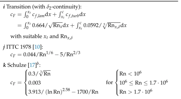
Table 2.Exemplary values for the viscous dragcFof a flat plate mentioned in the literature.xtis the position from the leading edge along the plate where the flow trips from laminar to turbulenta.
iTransition (withδ2-continuity): cF=
Rxt
0 cf,lamdx+ Rc
xtcf,turbdx
=Rxt 0 0.664/
√
Rnxdx+Rxct0.0592/p5 Rnx,δdx
with suitablextand Rnx,δ
jITTC 1978 [10]:
cF=0.044/Rn1/6−5/Rn2/3
kSchulze [17]b:
cF=
0.3/√3Rn
0.003
3.913/(ln Rn)2.58−1700/Rn for
Rn<106
106≤Rn≤1.7·106
Rn>1.7·106
aStreckwallet alspecify the Reynolds numbers of the transition pointx
tfor the open-water condition as 4·105(suction side)
and 2·105(pressure side), for the behind condition as 3·105(suction side) and 1·105(pressure side) [18].
bIn his presentation Schulze has an obvious misprint when giving the value of 0.03 for the middle part [17]. It should be
0.003 to assure continuity at its boundaries.
this paper this formulation was improved in such a way, that the local Reynolds number Rnx,δfor the
turbulent flow was adapted, so that in the transition point the impulse loss thicknessδ2is the same for
the laminar and the turbulent boundary layer (Schlichting [15]).
3.2. Form drag
The form dragc2dis the increase of the drag of a two-dimensional section when compared to the purely viscous drag of a flat plate. The reason for this increase is two-fold: Firstly, the flow velocity over the surface is higher due to the thickness of the profile increasing the viscous drag. Secondly, the pressure does not recover entirely due to losses in the boundary layer:
c2d=2∆cF+cP, (7)
where∆cF= relative increase of the friction due to the speed increase andcP= drag coefficient due to pressure losses.
The increase of the friction due to the higher velocity depends on the relative speed increase, the position of the transition point and the pressure gradient along the profile. For symmetrical sections the speed increase is the same for both sides and only depends on the thickness to chord ratiotmax/c. The position of the transition point depends on the Reynolds number, the turbulence of the inflow and the section shape. Values found in the literature for symmetrical profiles are given in Table3.
The pressure drag coefficientcPcan only be determined by analysing experimental results. It can be argued that it also depends on the position of the transition point, the pressure gradient and the occurrence of separation. Some values found in the literature for symmetrical profiles without flow separation are given in Table4.
4. Methodology
Since full scale open-water performance data for propellers are not easily attainable, the most straight-forward approach is to compare the power and shaft revolutions predicted from model tests with the values measured during full scale trials:
CP= PDT PDS
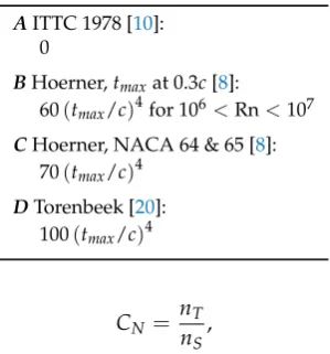
Table 3.Values for the relative form drag∆cF/(2cF)for symmetrical section profiles mentioned in the literature. For the NACA 64 & 65 laminar profiles the transition point was fixed at 0.09c. Hoerner also emphasises that the given relationship for these sections are only valid for rough surfaces [8].
AITTC 1978 [10]: 2tmax/c
BHoerner,tmaxat 0.3c[8]: 2tmax/cfor 106<Rn<107
CHoerner, NACA 64 & 65 [8]: 1.2tmax/c
DTorenbeek [20]: 2.7tmax/c
Table 4.Values for the relative pressure dragcP/(2cF)for symmetrical section profiles without flow separation mentioned in the literature. See also explanations given for Table3.
AITTC 1978 [10]: 0
BHoerner,tmaxat 0.3c[8]: 60(tmax/c)4for 106<Rn<107
CHoerner, NACA 64 & 65 [8]: 70(tmax/c)4
DTorenbeek [20]: 100(tmax/c)4
CN= nT nS
, (9)
whereCP,CN= model-ship correlation factors for the power and shaft speed,PDT,PDS= measured and predicted delivered power andnTandnS= measured and predicted shaft revolutions.
If the prediction methods were to be perfect, these two model-ship correlation factors would be 1 for every model test analysed But it is to be expected, that these factors scatter around a mean value, which is not necessarily 1. This shift in the mean value can be corrected by applying the model-ship correlation factor as a final step in the power prediction as stated in the ITTC 1978 method. A measure of the scatter is the standard deviation, which assumes that the distribution of values forms the bell shaped curve. The smaller the standard deviation the closer are the scattered values to the mean value, hence the better is the scaling method. Note that before calculating the standard deviation, the values must be normalized to give a mean value of 1.
The analysis was run by the Hamburgische Schiffbau-Versuchsanstalt (HSVA).1HSVA currently uses the strip method and previously used the Lerbs/Meyne [13] and the standard ITTC 1978 [10] methods, so these were already available. The βi-method was implemented by Stone Marine Propulsion (SMP), just as the ITTC method. This was necessary, so that the ITTC method can be used with different friction lines and form factors, which were implemented by SMP as well. Using this newly developed program, it was possible to calculate the open-water characteristics for the self-propulsion and full scale conditions for all possible combinations of scaling methods, friction lines and form factors.
1 Data processing was done solely at HSVA and results on trial predictions related to the various propeller scaling approaches
Based on HSVA’s databases of performance predictions and sea trials, the intersection of both sets was identified. The expected power was calculated according to HSVA’s standard performance prediction method (see section 4.1).
The 25 scaling methods used are summarized in Table5. The finished roughnesskof the propeller in full scale was assumed to be 20µm.
Table 5.Scaling methodsλinvestigated. A mark in theR
-columns denotes that the scaling procedure integrates the sectional friction over the whole blade. The capital letters specifying the friction lines, form and pressure drag are references to the Tables1&2,3and4, respectively (OW = open-water, SP = self-propulsion and FS = full scale). The finished roughnesskof the propeller in full scale was assumed to be 20µm.
Friction lines Drag
Method R
OW SP FS Form~ Pressure~
A ITTC j j h A A
B ITTC j — h A A
C ITTC × j j h A A
D ITTC × j — h A A
E ITTC j j f A A
F ITTC j — f A A
G ITTC × j j f A A
H ITTC × j — f A A
I ITTC e e e incl. A
J ITTC e — e incl. A
K ITTC i i i A A
L ITTC k k g D D
M Meyne — — — — —
N Strip × e e e incl. A
O Strip × e — e incl. A
P βi j j h A A
Q βi j — h A A
R βi × j j h A A
S βi × j — h A A
T βi j j f A A
U βi j — f A A
V βi × j j f A A
W βi × j — f A A
X βi i i i A A
Y βi × i i i A A
4.1. Performance prediction method
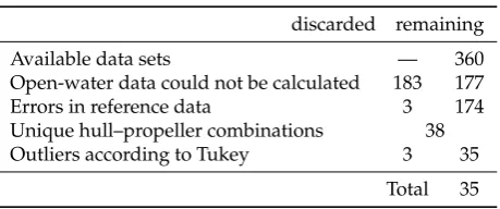
Table 6.Number of used data sets.
discarded remaining
Available data sets — 360
Open-water data could not be calculated 183 177
Errors in reference data 3 174
Unique hull–propeller combinations 38
Outliers according to Tukey 3 35
Total 35
necessary) to include appendages and hull openings not present during the model tests. The thrust correction causes adequate power and shaft speed adjustments for the sea trials, achievable by the aid of the propeller open-water diagram.
4.2. Analysis
The intersection of performance predictions and sea trials available at HSVA consisted of 360 data records (see Table6). For 183 records the open-water characteristics could not be calculated for all scaling methods considered. By visual inspection it was found that three sets have an obvious mistake in either the available trial or prediction data. The remaining 174 data sets consist of 38 unique propeller-hull configurations. The mean values ofCPandCNwere calculated for each of these configurations using each of the 25 propeller scaling methods listed in Table5. Finally the resulted distribution was filtered according to Tukey’s range test: If for one data set more then half of the CPvalues are outside Tukey’s range calculated with the typical value ofk= 1.5, this data set was disregarded. The Tukey’s range for valid data points was calculated with:
Q1,λ−k(Q3,λ−Q1,λ)<CP,i,λ<Q3,λ+k(Q3,λ−Q1,λ), (10)
whereQ1,λandQ3,λ= lower and upper quartiles of allCPvalues for one scaling methodλ.
Using these valid 35 data sets, the following values were calculated for each scaling methodλ:
• Mean value of all data sets for each scaling methodλ:
CP,λ=
1 N
N
∑
i=1
CP,i,λ, (11)
• Normalized model-ship correlation factors:
C∗P,i,λ= CP,i,λ CP,λ
, (12)
• Standard deviationSPof all normalized data sets for each scaling methodλ:
S∗P,λ= v u u t1
N N
∑
i=1
C∗P,i,λ−12, (13)
whereN= number of valid data sets andCP,i,λ= model-ship power correlation factor for theithdata
set. Note that the normalized mean valuesC∗P,λare always 1.
C
P,λCP,λ [–]
0.98 1 1.02 1.04 1.06 1.08 1.1
S
ca
lin
g
m
et
h
od
A+B C+D E+F G+H I+J K L M N+O P+Q R+S T+U V+W X Y
Figure 2.Mean valuesCP,λof the model-ship power correlation factorsCP,λfor all scaling methodsλ. If the same scaling method was investigated with and without scaling to the Reynolds number of the self-propulsion test, the results are grouped together; the black bar stands for the no scaling to the self-propulsion test. The capital letters reference Table5.
5. Results
The mean valuesCP,λof the model-ship power correlation factorsCP,ifor each propeller scaling methodλ (equation11) are shown in Figure2. It should be noted that a mean value of 1 is not necessarily an indicator for the quality of the propeller scaling method.
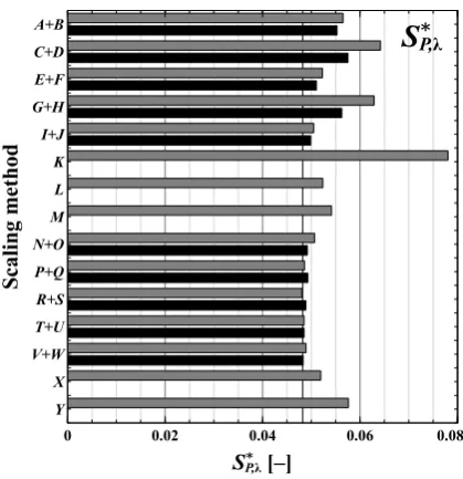
Figure3shows the standard deviationS∗P,λ of the normalized model-ship power correlation factorsC∗P,i,λ(equation13).
The following patterns can be seen in the Figures2and3:
1. The mean values of the model-ship power correlation factor is about 1 for most investigated scaling methods.
2. The scaling methods which do not scale down to the Reynolds number of the self-propulsion test typically perform better than the same method using the scaled down open-water characteristics to analyse the self-propulsion test (B–A,D–C,F–E,H–G,J–I,O–N,Q–P,U–TandW–V, but not S–R).
3. The methods using the original Schlichting friction line f for the full scale propeller tend to perform better (E–A,F–B,G–C,H–D,T–PandW–S, but notU–QandV–R).
4. All methods using the local surface frictionitrying to capture the transition from laminar to turbulent flow do not perform very well (K,XandY).
5. Theβi-methods integrating the friction forces over the whole blade perform better than the same method using only the friction force of a significant profile (R–P,S–Q, andW–U, but notV–T and the notable exceptionY–X). For the ITTC 1978 methods this trend is reversed (C–A,D–B, G–EandH–F).
6. The most recent methods perform better than the original ITTC 1978 methodA.
7. Theβi-methodsRandWintegrating the ITTC 1978 and Schlichting friction lineshandf over
S
∗P,λS
ca
lin
g
m
et
h
od
A+B C+D E+F G+H I+J K L M N+O P+Q R+S T+U V+W X Y
S∗P,λ [–]
0 0.02 0.04 0.06 0.08
Figure 3. Standard deviationS∗P,
λ of the normalized model-ship power correlation factorC ∗ P,ifor all scaling methodsλ. If the same scaling method was investigated with and without scaling to the Reynolds number of the self-propulsion test, the results are grouped together, the black bar stands for no scaling to the self-propulsion test. The capital letters reference Table5.
6. Discussion
The scaling approaches compared in this paper rely on the estimates of the normalized drag forces experienced by either a single section representing the blade or – in the integral cases, such as the strip method – by individual sections building up the blade. All methods but the Meyne andβi-methods
consider the resistance force vector to be orientated in the direction of the nose-tail line; both the Meyne and theβi-method calculate the direction of the hydrodynamic inflow and aligns the resistance force parallel to it. In terms of a favourable standard deviation of the normalized power correction factorCP∗, the quality of a specific approach is also linked to the qualities of the drag estimates achieved in model or full scale. The ability to account correctly for local Reynolds number variations, either in the model or full scale Reynolds number region, would be reflected in a lower standard deviation.
Generally it can be considered more challenging to capture Reynolds number sensitivities in the model scale case due to the extended presence of laminar flow over the model propeller blade. Referencing item2from the list presented in section 5, it could be concluded that none of the used friction lines is able to predict the friction forces in model scale accurately. Better results are achieved by using the open-water data without any correction applied to analyse the self-propulsion test. One possible reason for this behaviour might lie in the fact, that the inflow into the propeller during the self-propulsion test is more turbulent due to the boundary layer of the ship model than during the open-water test. This turbulent inflow would trigger an earlier transition from laminar to turbulent flow similar to the open-water test in undisturbed inflow.
The data presented indicates that for full scale the original Schlichting friction linef might be a good choice for any scaling procedure.
C
∗(ITTC)N,i,λ
C
∗
(I
T
T
C
)
N
,i,
λ
0.96 0.98 1 1.02 1.04
Data Set Nº
0 25 50 75 100 125 150 175
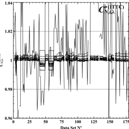
Figure 4.C∗N(ITTC),i,
λ of the model-ship shaft speed correlation factorsCN,i,λnormalized with the ITTC 1978 propeller scaling methods. The small scatter around the value of 1 indicates a small influence of the propeller scaling method on the prediction of the shaft speed.
It should be mentioned that the strip methodN has the advantage to have been confirmed previously by quite the same data set used in this investigation to analyse all scaling methods.
All propeller scaling methods investigated in this paper are supposed to show negligible differences in view of their influence on the full scale shaft speed prediction. Consequently the isolated sensitivity of the shaft speed forecast on the traditional propeller scaling approaches is to be considered minor. This can be shown by calculating the ratios
CN∗(ITTC),i,λ = CN,i,λ CN,i,λ=ITTC
, (14)
whereCN,i,λ=ITTC= model-ship correlation factor for the shaft speed calculated using the ITTC 1978
propeller scaling methodA. A ratio close to 1 for all propeller scaling methods indicates a minor sensitivity ofCN,i,λ, which is shown in Figure4for all 177 valid data sets used in this investigation.
This confirms that the predictions for the shaft speed are hardly a matter of propeller scaling contrary to the power predictions.
7. Conclusions
The power and shaft revolutions were predicted by the standard HSVA performance prediction method but with 25 different propeller scaling methods. These predictions were compared to the measured trials data to quantify the quality of each propeller scaling method. The standard deviations of the normalized model-ship power correlation factors were calculated as a measure of the quality of the prediction. All investigated methods showed a mean value of this correlation factor of about 1.
From the data available the most promising friction line for the full scale propeller is the original Schlichting linef.
From the propeller scaling methods investigated, theβi-method in its variantsRandW, where the friction forces are integrated over the whole blade, showed the best results. The most likely reason is, that this method aligns the drag forces with the actual hydrodynamic inflow angle experienced by the propeller blade and that it does not need to know the sectional form drag.
It might be worthwhile to investigate numerical methods to calculate the section drag, such as outlined by Thwaites [19] and Head [5]. Drela implemented the transition from laminar to turbulent flow in the software XFoil [3]. The values for the section drag calculated numerically can be used by any scaling method investigated in this paper.
It must be mentioned, that the original 360 trial data sets were reduced to just 35 unique propeller–hull combinations due to rigorous data checks and averaging over sister-ship cases. HSVA is currently investing in a maintenance program for the database to allow for an enlargement of data sets, which would pass the rigorous consistency checks.
With more data available, it becomes feasible to run an optimization on a parametrized friction line with the target to further minimize the scatter of the model-ship power correlation factors.
In the current investigation the influence of different formulations of the form and pressure drags was not investigated.
Finally it must be noted, that no unconventional propellers, such as end-plate, tip-raked propellers or propellers with unconventional section shapes, such as the NPT propeller, were present in the data sets available to the current investigation. Because of the underlying physical principles, it can be assumed, that theβi-methods integrating the friction forces over the whole blade will also perform best for these propellers. When unconventional propellers are included in such investigations, one should be aware that their number is very small compared to more conventional designs, hence their influence on the overall outcome is most likely negligible. Since most newly developed propeller scaling methods claim to be give more accurate results for unconventional propellers, this group of propellers must be looked at separately to isolate the effect of different propeller scaling methods.
8. Final Note
The software developed to calculate the scaled open-water characteristics is published with an open license on the principal author’s GitLab websitehttps://gitlab.com/sphh/PyOWscaling. All functionality are realized as plug-ins written in Python. It is easy to write your own plug-in to implement other propeller scaling methods, friction lines and in- and output formats. It will be appreciated, if you made your plug-ins available to the public.
Author Contributions:The idea of this paper emerged during discussions between Stephan Helma and Heinrich Streckwall. Jan Richter set up and run the power predictions. Heinrich Streckwall contributed the computer code for the strip method, parts of the manuscript, preliminary post processing and evaluated the data filtering. Stephan Helma contributed the computer code for the other scaling methods. He did the data filtering, the final post processing and wrote most of the manuscript.
Abbreviations
The following abbreviations are used in this manuscript:
CFD Computational Fluid Dynamics
FS full scale
HSVA Hamburgische Schiffbau-Versuchsanstalt GmbH ITTC International Towing Tank Conference
ITTC 1978 ITTC Performance Prediction Method [10]
OW open-water
SMP Stone Marine Propulsion Ltd. SP self-propulsion
Appendix. Review of ITTC 1978 scaling procedure
The total propeller forceFcan be composed from the propeller thrustTand torqueQ
F2=T2+ Q xD2
!2 ,
wherex= fractional lever of the torque, which does not change with the scaling. This relation can be make dimensionless by dividing by ρn2D42:
K2F =K2T+ 4 x2K
2 Q.
Using the ITTC 1978 [10] scaling forKTandKQ
∆KT =0.3∆cD P D
c DZ,
∆KQ=−0.25∆cD c DZ, it is possible to scale the propeller force coefficient:
K0F2 = K0T2+ 4 x2K
0 Q
2
= (KT+∆KT)2+ 4
x2 KQ+∆KQ 2
=
KT+0.3∆cDP D
c DZ
2 +
+4 x2
KQ−0.25∆cD c DZ
2 .
Hence
K0F =f(KT,KQ,∆cD c DZ,
P D),
which shows that the scaled propeller force is not only a function of the thrust and torque figures and the increase in section drag∆cDZc/D, but also of the pitch to diameter rationP/D. In the opinion of the authors this dependency cannot be explained with first principles. This surprising result is a property of all scaling methods which are based on the ITTC procedure.
References
1. Abbott, I.H. & von Doenhoff, A.E. em Theory of Wing Sections; Dover Publications, Inc: New York, USA, 1959.
2. Brown, M., Sanchez-Caja, A., Adalid, J.G., Black, S., Sobrino, M.P., Duerr, P., Schroeder, S. & Saisto, I. Improving Propeller Efficiency Through Tip Loading.30thSymposium on Naval Hydrodynamics2014, Hobart, Tasmania, Australia.
3. Drela, M. em XFoil Subsonic Airfoil Development System;http://web.mit.edu/drela/Public/web/xfoil/, 2013.
4. Hasuike, N., Okazaki, M. & Okazak, A. ‘Flow characteristics around marine propellers in self propulsion test condition’.19thNumerical Towing Tank Symposium (NuTTS’16)2016, St Pierre d’Oléron, France. 5. Head, M.R. ‘Entrainment in the Turbulent Boundary Layer’.Aeronautical Research Council Report1958, R&M
3152.
7. Helma, S. ‘A scaling procedure for modern propeller designs’.Ocean Engineering2016,120, pp. 165-174. 8. Hoerner, S.F.Fluid-Dynamic Drag, theoretical, experimental and statistical information; Hoerner Fluid Dynamics:
Bakersfield, USA, 1965 (reprint).
9. ITTC. ‘Resistance Test’.ITTC – Recommended Procedures and Guidelines1957, Effective Date 2011, Revision 03. 10. ITTC. Propulsion Committee of 27th ITTC 2014. ‘1978 ITTC Performance Prediction Method’. ITTC –
Recommended Procedures and Guidelines1978, Effective Date 2014, Revision 03.
11. von Kármán, Th. ‘Turbulence and Skin Friction’.J. of the Aeronautical Sciences1934,1, No. 1, pp. 1-20. 12. Kuiper, G.The Wageningen Propeller Series; MARIN: Wageningen, The Netherlands, 1992.
13. Meyne, K. ‘Untersuchung der Propellergrenzschichtströmung und der Einfluss der Reibung auf die Propellerkenngrößen’.STG-Jahrbuch1972, Hamburg, Germany.
14. Praefke, E. ‘Multi-Component Propulsors for Merchant Ships – Design Considerations and Model Test Results’.SNAME Symposium “Propeller/Shafting’94”1994, Virginia, USA.
15. Schlichting, H. & Gersten, K.Grenzschicht-Theorie; Springer Verlag: Berlin, Germany, 2006.
16. Schönherr, K.E. ‘Resistance of Flat Surfaces Moving Through a Fluid’.SNAME Transactions193240, pp.279. 17. Schulze, R. ‘Neue Verfahren zur Reynoldszahlkorrektur für Freifahrtmessungen an Modellpropellern’.
PresentationSTG-Sprechtag „Moderne Propulsionskonzepte”2016, Hamburg, Germany.
18. Streckwall, H., Greitsch, L., Müller, J., Scharf, M. & Bugalski, T. ‘Development of a Strip Method Proposed as New Standard for Propeller Performance Scaling’.Ship Technology Research2013,60, pp. 58–69.
19. Thwaites, B. ‘Approximate Calculation of the Laminar Boundary Layer’. Aeronautical Quarterly1949,1, November 1949.
20. Torenbeek, E. ‘Synthesis of Subsonic Airplane Design’.The Netherlands and Martinus Nijhoff1992, Delft Univ. Press, Delft, The Netherlands.