Measuring Strategic Communications

(1)

University of South Carolina

Scholar Commons

Theses and Dissertations

6-30-2016

Visibility-Based Pursuit-Evasion In The Plane

Nicholas Michael Stiffler

University of South Carolina

Follow this and additional works at:https://scholarcommons.sc.edu/etd Part of theComputer Engineering Commons

This Open Access Dissertation is brought to you by Scholar Commons. It has been accepted for inclusion in Theses and Dissertations by an authorized administrator of Scholar Commons. For more information, please [email protected].

Recommended Citation

Stiffler, N. M.(2016).Visibility-Based Pursuit-Evasion In The Plane.(Doctoral dissertation). Retrieved from

(2)

Visibility-Based Pursuit-Evasion in the Plane

by

Nicholas Michael Stiﬄer

Bachelor of Science

University of South Carolina, 2009 Master of Science

University of South Carolina, 2012

Submitted in Partial Fulﬁllment of the Requirements

for the Degree of Doctor of Philosophy in

Computer Science and Engineering

College of Engineering and Computing

University of South Carolina

2016

Accepted by:

Jason M. O’Kane, Major Professor

Marco Valtorta, Committee Member

Michael N. Huhns, Committee Member

Manton M. Matthews, Committee Member

Linyuan Lu, External Committee Member

(3)

c

Copyright by Nicholas Michael Stiﬄer, 2016

(4)

Dedication

“The true test of a man’s character is what he does when no one is watching.”

– John Wooden

For my siblings

Tyler, Lydia, Kyle, Jordan, and Blue

(5)

Acknowledgments

This thesis is the culmination of several years of scholarship and would not have been

possible without the generous contributions of many diﬀerent people. My mentor,

Jason O’Kane, had the most profound impact on my development as a research

scientist and provided valuable advice along the way.

I also oﬀer sincere thanks to my peers in theSouthCarolinaAutonomousRobotics

Research (SCARR) group: Mohammad Behbooei, Laura Boccanfuso, Shervin

Ghasem-loo, Jeremy Lewis, Fatemeh Zahra Saberifar, and Yang Song. The research group

fostered a fertile environment in which I was able to do my best work. My committee

members Michael Huhns, Linyuan Lu, Manton Matthews, and Marco Valtorta oﬀered

helpful guidance throughout by applying their unique expertise and perspective to

my work. Ioannis Rekleitis, while not a serving member of my committee, also

de-serves recognition for his willingness to provide an external perspective on my work.

Many other faculty and professors, including Ryan Austin, Randy Baldwin, Jenay

Beer, Duncan Buell, Stephen Fenner, Srihari Nelakuditi, Barb Ulrich, and Gabriel

Terejanu, have had immense inﬂuence on my growth and development as a computer

scientist and as a person. Thank you for the the various contributions you each have

made to my life.

More personally, I am thankful for the love and support that I have received from

my family and friends during my time in graduate school. Thank you to David and

Chelsea Hilmer, Matthew Crocket, Spencer Childress, Michael and Katie Reynolds,

and Conway “Deuce” Harris, whose friendship during this arduous journey was pivotal

(6)

Finally, it would be impossible to describe the amount of loving support and

en-couragemnt I’v recieved from my ﬁance, Lacie. Thank you for tolerating me

through-out this journey.

Financial support for this work was provided by the NSF under award IIS-0953503

(7)

Abstract

As technological advances further increase the amount of memory and computing

power available to mobile robots, we are seeing an unprecedented explosion in the

utilization of deployable robots for various tasks. The speed at which robots begin to

enter various domains is largely dependent on the availability of robust and eﬃcient

algorithms that are capable of solving the complex planning problems inherent to

the given domain. One such domain which is experiencing unprecedented growth in

recent years requires a robot to detect and/or track a mobile agent or group of agents.

In these scenarios, there are typically two players with diametrically opposed

goals. For matters of security, we have a guard and an intruder. The guard’s goal is

to ensure that if an intruder enters the premises they are caught in a timely manner.

Analogously, the intruder wishes to evade detection for as long as possible. Search

and rescue operations are often framed as a two-player game between rescuers and

survivors. Though the survivors are unlikely to behave antagonistically, an agnostic

model is useful for the rescuers to guarantee that the survivors are found, regardless

of their movements. Both of these tasks, are at their core, pursuit-evasion problems.

There are many variants of the pursuit-evasion problem, the common theme

amongst them is that one group of agents, the “pursuers”, attempts to track

mem-bers of another group, the “evaders”. Geometric formulations of the pursuit-evasion

problem require a pursuer(s) to systematically search an environment to locate one

or more evaders ensuring that all evaders will be captured by the pursuer(s) in a

ﬁnite time. Thevisibility-based pursuit-evasion problem is a geometric variant of the

(8)

re-gion of the environment that the pursuer(s) can actively perceive. If an evader lies

within this visibility region then it is captured (detected).

This thesis contains four novel contributions that solve various visibility-based

pursuit-evasion problems. The ﬁrst contribution is an algorithm that computes the

optimal (minimal path length) pursuer trajectory for a single pursuer. The

sec-ond contribution is an algorithm that generates a joint motion strategy for multiple

pursuers. Motivated by the result of the second contribution, the third result is a

sampling-based algorithm for the multiple pursuer scenario. The fourth contribution

is a complete algorithm that computes a trajectory for a pursuer that has a very

(9)

List of Tables

Table 5.1 Table that corresponds to a pursuer making repeated crossings over an Appear/Disappear event boundary. Scenarios 1 and 2 consider when a disappear event occurs ﬁrst whereas Scenario 3

describes what occurs when an appear event occurs ﬁrst. . . 52

Table 5.2 Table that corresponds to a pursuer making repeated crossings over a Split/Merge event boundary. Scenarios 4-7 detail the various PEG-nodes that are visited when the merge event occurs ﬁrst. 53 Table 5.3 Table that corresponds to a pursuer making repeated crossings over a Split/Merge event boundary. Scenarios 8 and 9 consider when a merge event occurs ﬁrst. . . 53

Table 5.4 The simulation results for the GL3_{M algorithm, GL}3_{M with} post-processing ToS path smoothing, and our optimal algorithm. . 60

Table 6.1 The ten possible shadow vertex merges can be grouped into four general cases. . . 68

Table 7.1 Simulation Results for the brick environment. . . 94

Table 7.2 Simulation Results for the H environment. . . 95

(12)

List of Figures

Figure 1.1 The basic motion planning problem visualized using the concept of conﬁguration space. The task is to ﬁnd a collision free path

inCfree from qI toqG. . . 8

Figure 1.2 Organization of this thesis with arrows indicating dependencies.

Novel results are denoted by the shaded blocks. . . 12

Figure 2.1 An environment with two pursuers (red circles) and three

shad-ows (ﬁlled path-connected regions). . . 18

Figure 2.2 An appear event increases the number of shadows by one, and the new shadow is labelled clear (green region). A disappear

event decreases the number of shadows, its label is discarded. . . 22

Figure 2.3 When a shadow splits into multiple shadows, they inherit the same label as the original shadow. When a merge event occurs the new shadow is clear if and only if all of the original shadows

are also clear. . . 23

Figure 2.4 A push event occurs when a shadow gets pushed between

neigh-boring pairs of environment reﬂex vertices. . . 24

Figure 4.1 An illustration of the concept of conservative regions. . . 32

Figure 4.2 Ray shooting is performed for three general cases to form the

conservative regions. . . 33

Figure 4.3 An example of the Pursuit Evasion Graph for a given environment. 34

Figure 5.1 A single Shortest Path Map. These four rays and one segment subdivide the plane into regions with combinatorially equivalent

(13)

Figure 5.2 The SPM for the ﬁrst segments divides the plane according to the combinatorial structure of the shortest path from p tos to

a query point q. . . 42

Figure 5.3 Computing the Shortest Path Map for segment si depends on

the Shortest Path Map for segmentsi−₁. . . 44

Figure 5.4 The scenario that occurs when theUnavailingPruning strat-egy is used. Initially the pursuer must travel to the closest critical boundary edge. Then for sequences of even length the pursuer will be in the blue conservative region. For sequences

of odd length, the pursuer will be in the green conservative region. 50

Figure 5.5 An environment (5.5a) where the optimal pursuer strategy (5.5b) returned by our algorithm looks vastly diﬀerent from both the original GL3_{M strategy (5.5c) and the GL}3_{M strategy optimized}

using a ToS (5.5d). . . 62

Figure 5.6 An environment (5.6a) where the optimal pursuer strategy (5.6b) returned by our algorithm looks fairly similar to both the orig-inal GL3_{M strategy (5.6c) and the GL}3_{M strategy optimized}

using a ToS (5.6d). . . 63

Figure 5.7 An environment (5.7a) where the optimal pursuer strategy (5.7b) returned by our algorithm looks vastly diﬀerent from both the original GL3_{M strategy (5.7c) and the GL}3_{M strategy optimized}

using a ToS (5.7d). . . 64

Figure 6.1 A conﬁguration of three robots searching an environment. The

shaded regions represent areas hidden to the pursuers. . . 66

Figure 6.2 An environment with two pursuers illustrating the diﬀerent

types of shadow vertices. . . 67

Figure 6.3 Type I and Type III vertices merge into a Type III vertex. . . 68

Figure 6.4 A Type II vertex merges with a Type III vertex, eliminating

the shadow. . . 69

Figure 6.5 A Type II vertex merges with a Type IV vertex, creating a

Type III vertex. . . 70

Figure 6.6 A Type III vertex merges with a Type III vertex creating a

(14)

Figure 6.7 A Type III vertex merges with a Type IV vertex, creating a

Type III vertex. . . 71

Figure 6.8 A Type IV vertex merging with a Type IV vertex with 2-robots. . 72

Figure 6.9 A Type IV vertex merging with a Type IV vertex requires

mul-tiple robots and creates a single Type IV vertex. . . 73

Figure 6.10 Merge events that never occur: (a) I-I (b) I-II (c) I-IV (d) II-II. . 74

Figure 6.11 An example of a critical boundary(bitangent) polynomial pass-ing through obstacles. Because the pursuer motion shown crosses this boundary, it moves to a new CAD cell, even though no

shadow event occurs. . . 76

Figure 7.1 A pursuer strategy generated by our algorithm. Filled circles represent the pursuers’ initial positions and open circles

repre-sent their goal positions. . . 80

Figure 7.2 A snapshot of the SG-PEG. Dashed red lines indicate a unique

joint pursuer conﬁguration. . . 82

Figure 7.3 An illustration of the update step. Initially there are two con-taminated shadows (purple). During the Update a new label appears. At the conclusion of the Update method, there are two shadows: a cleared shadow (green) and a contaminated

shadow (purple). . . 83

Figure 7.4 By considering only straight line motions that do not intersect

the environment we ensure the generation of collision free strategies. 88

Figure 7.5 Multiple intermediary vertices are preferred to a single long

connection. . . 88

Figure 7.6 A collection of dense samples is problematic since cycles can occupy a large amount of computing resources. To combat this

we can require all cycles to be a minimum length. . . 89

(15)

Figure 8.1 A pursuit plan (left) computed by our algorithm. The pursuer uses four orthogonal beams (right) to capture the evader, re-gardless of the evader’s path or velocity. The pursuer starts on the bottom boundary of the top-center corridor, and travels

ﬁrst to the left and then to the right. . . 98

Figure 8.2 A robot with four ﬁxed beam sensors. In this example gap g12

is shaded green. . . 102

Figure 8.3 An illustration to detect when a Left event occurs. An

illus-tration to detect when a Right event occurs. . . 103

Figure 8.4 An illustration that demonstrates when an event does not occur at a reﬂex vertex. An illustration that demonstrates when an

event does not occur at a convex vertex. . . 103

Figure 8.5 Decomposition of a simple environment into conservative

re-gions by ray extensions. . . 105

Figure 8.6 Reﬁnement of the decomposition from Figure 8.5 by vertical ray extensions upward and downward from each vertex. The

resulting cells are convex. . . 106

Figure 8.7 An illustration of theLeft Extend/Retract events. . . 107

Figure 8.8 An illustration of theRight Extend/Retract events. . . 107

Figure 8.9 A scenario where gap edges can appear/disappear and shrink/grow. When travelling from the interior to the boundary edgeg01and g40disappear,g12andg34shrink toge2 and g3e, andg23remains

the same. Conversely, when travelling from the boundary edge

to the interior gap edges appear, grow, and remain the same. . . . 109

Figure 8.10 An illustration of thesplit andmergeevents that occur when

transitioning between an edge of the region graph and an

envi-ronment vertex. . . 110

Figure 8.11 The ﬁnal generated plan for the example shown in Figures 8.5

and 8.6. . . 112

Figure 8.12 A plan generated by our algorithm for the above environment. . . 112

Figure A.1 An environment described by four polynomials and it’s

(16)

Figure A.2 The CAD of the gingerbread face and the adjacency graph

(17)

Chapter 1 Introduction

One of the ultimate goals in Robotics is the creation of an autonomous system that

is capable of converting high-level task speciﬁcations from humans into low-level

descriptions detailing how to accomplish the task. Planning algorithms are

instru-mental in creating autonomous systems. A planning algorithmautonomously decides

the sequence of actions necessary to perform a task given an initial conﬁguration, a

collection of goal conﬁgurations, and a collection of sensors. This may appear to be

a relatively straightforward process, but challenges such as eﬀectively modelling the

planning problem and designing and implementing eﬃcient algorithms complicate the

process.

The motion planning problem is a reﬁnement of the planning problem. At the

highest level, the motion planning problem asks the following question; “How can a

robot decide what motions to perform in order to achieve its goal while operating

in the physical world?” In the context of Robotics, the motion planning problem

appears in such problems as: navigation, coverage, localization, manipulation, and

pursuit-evasion.

In this thesis we focus on the pursuit-evasion problem. Although there are many

variants of the pursuit-evasion problem, the common theme amongst them is that

one group of agents, the pursuers, attempts to systematically locate the members

of another group, the evaders. Pursuit-evasion problems are of particular interest

because surveillance, evasion/detection, and search and rescue (SAR) are, at their

(18)

mentioned problems can be interpreted as pursuit-evasion problems.

• In a surveillance problem such as the Art Gallery Problem1 _{[64], the guards can}

be represented as mobile robots equipped with a camera and tracking software.

• An evasion/detection problem where one agent wants to remain hidden/undetected

from another adversarial agent can also be adapted to incorporate a robot. A

robot similar to the one used in the hypothetical surveillance scenario can act

as the adversary in this instance.

• Another scenario that beneﬁts from deployable robots are search and rescue

operations during a disaster. Rather than exacerbate the situation by placing

the rescuers in harm’s way, an alternative strategy exists where a team of

au-tonomous search and rescue robots conduct the rescue operation. By framing

the scenario in the context of a pursuit-evasion game where the evaders are

the survivors and the pursuers are the robots, we can utilize the algorithms

developed to solve pursuit-evasion problems to aid in rescue operations.

This is but a small sample of potential scenarios that illustrate the presence of

pursuit-evasion problems in the real world. It is imperative that we ﬁnd eﬀective ways in

which to tackle these problems.

The remainder of this introductory chapter is organized into two parts. The ﬁrst is

a brief overview of motion planning (Section 1.1), and the second contains a preview

of the primary results and overall structure of the thesis (Section 1.2).

1

(19)

1.1 Motion Planning

This section is not designed to be a comprehensive guide to motion planning. Indeed,

entire books [17, 46, 47] have been written on the subject. Instead, this section aims

to provide enough details so that the reader is left with a clear understanding of what

entails a motion planning problem, and the general tools/mechanisms used to tackle

these kinds of problems.

1.1.1 Basic Ingredients of Planning

This section contains several basic ingredients that appear in motion planning.

Al-though this thesis focuses on the pursuit-evasion problem, the following apply to

nearly all motion planning problems regardless of topic.

States

A crucial idea that is the foundation of any motion planning problem is the concept

of a state.

Definition 1. Astateis the collection of all aspects of the robot and the environment

that can have an impact on the future.

The state is a complete description of the robot’s physical situation in the

environ-ment. A single state represents just one possible representation of the robot. The set

of all possibles states is called the robot’s state space. The notation x ∈ X is often

used to denote a speciﬁc state in the robot’s state space.

Actions and Transitions

Robots interact with and move through the environment by changing their state,

(20)

Definition 2. An action, also known as inputs or controls in control theory, is any

physical interaction that causes a change to the robot’s state.

An action in this case is a robot initiated physical interaction. The set of all possible

actions that the robot can take is called the robot’s action space. A robot action is

typically denoted asu∈U, whereu is a single action belonging to the robot’s action

space, U.

Equipped with a formal way to represent a robot’s situation in the environment

and a set of possible ways in which the robot can act upon the environment we can

formally discuss how a robot goes about changing its state through the use of astate

transition function.

Definition 3. A state transition function is a function whose input is a state xk and

an action uk and outputs a state xk+1 for any timek ≥0.

In its simplest form, the state transition function is a mathematical representation

detailing how a robot updates its state during execution by “transitioning” from one

state to another until a goal state is reached. Mathematically, the state transition

function appears as

f :X×U →X

xk+1 =f(xk, uk).

(1.1)

Observations

A central idea in Robotics is the ability for a robot to infer knowledge about itself

and/or its surroundings through the use of sensors. The key idea is that any

infor-mation that we want to utilize to inﬂuence the control of the robot must come from

sensors. In a perfect scenario, a sensor provides complete information. This involves

avoiding ambiguity by yielding complete information, utilizing noiseless sensors, and

using simple enough sensors that they are easy to model. Often times sensors provide

(21)

For this thesis, we will focus on how to represent a robot’s available sensory data

in the context of the models discussed in this section.

Definition 4. Anobservation is all of the current available sensor information that

the robot has access to.

At its core, the observation provides the robot with a “hint” about what the current

state is. An observation is typically denoted asy∈Y, wherey is a single observation from the observation space. Since the observation is dependent on the robot’s current

state, the observation function appears as

h:X →Y

y=h(x).

(1.2)

Note that the robot need not necessarily know the state used to generate a particular

observation.

Representing the Passage of Time

There are a number of ways to represent the passage of time, the following three

representations are the most prevalent: continuous time, discrete time with a ﬁxed

length, and discrete stage with variable length. The choice of model is often dependent

on the application. We focus on the continuous time and discrete stage models in

this thesis.

In the continuous time model, time is represented by a real number t. The robot

can potentially change its action at any instant in time, thus the robot’s actions

can be expressed as a function u(t) of time. The state transition function in the

continuous time domain takes the derivative of the state with respect to time and

appears as dx

dt = f(x, u) or alternatively ˙x = f(x, u). The new state can then be computed via integration x(t) =

t

R

0f

x(s), u(s)ds.

In the discrete stage time model, time progresses in a series of discrete stages, that

(22)

time is represented by a stage counterkrather than a physical time. This higher level model allows for more abstract actions in the sense that you can perform an action

u for any desired duration. The transition function for the discrete stage model is

essentially the same one introduced in Equation 1.1, that isxk+1 =f(xk, uk).

Representing Uncertainty

In this context uncertainty refers to the situation where the robot is unsure of its

current state. Uncertainty in a system can be attributed to several factors;

uncer-tain actions, unceruncer-tain sensing, and initial unceruncer-tainty. We model this ambiguity by

introducing an adversary called “nature” which interferes with the robot by adding

noise to the system. In this way we can adapt the models used up to this point by

introducing nature actions and observations to account for any uncertainty that may

exist in our system. Nature actions are denoted as θ ∈ Θ, where Θ is the nature action space. The introduction of nature actions requires the following modiﬁcation

to our state transition function in Equation 1.1:

f :X×U ×Θ→X

xk+1 =f(xk, uk, θk).

(1.3)

Two reasonable models for interpreting the value of θ that nature chooses are

nonde-terministic and probabilistic models. The nondenonde-terministic model can be viewed as

the worst-case scenario model where we don’t know anything about howθ is chosen,

whereas the probabilistic model assumes that nature chooses θ according to some probability distribution.

We can also assume that nature interferes with our robot’s observations as well.

Nature observations are denoted as ψ ∈Ψ, where Ψ is the nature observation space.

(23)

func-tion in Equafunc-tion 1.2 to:

h:X×Ψ→Y

y=h(x, ψ)

(1.4)

Our time models can be adapted to account for the eﬀects of nature. The action

errors cause the continuous time state transition function to become ˙x = f(x, u, θ) and the discrete stage state transition function to becomexk+1 =f(xk, uk, θk). Simi-larly, sensing errors require a modiﬁcation to the observation functions. The

contin-uous time observation function becomes y(t) = hx(t), ψ(t) and the discrete stage

observation function becomes yk =h(xk, ψk).

Configuration Spaces

This section provides a high level introduction toconfiguration spaces. The key idea is

that we want to represent the robot as a single point in the appropriate space, and by

extension seek a mapping that transforms obstacles into an appropriate representation

in this space. This space is called the robot’s conﬁguration space, also commonly

referred to as the C-space. A configuration is a single point in the conﬁguration

space.

Definition 5. A configuration is a complete speciﬁcation of the position of every

point in the system.

By considering a problem in the robot’s C-space, we can transform the problem

of planning the motion of a spatial object into the problem of planning the motion

of a point. At its core, the C-space is just a special kind of state space.

Now we attempt to provide some intuition concerning the transformation of a

general path planning problem into a problem in the robot’s C-space. Informally,

we want to shrink the robot down to a point and expand the obstacles by the same

(24)

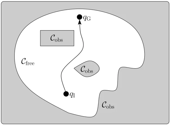
q

G

q

I

C

_free

C

_obs

C

_obs

C

_obs

Figure 1.1: The basic motion planning problem visualized using the concept of con-ﬁguration space. The task is to ﬁnd a collision free path in Cfree fromqI to qG.

of the expanded obstacle region in the C-space, then the corresponding spatial robot

will stay out of the real workspace obstacles.

The C-space is just a collection of possible conﬁgurations that our robot could

occupy. However, similar to the physical domain there are areas of the C-space called

obstacle configurations that we want to restrict the robot from entering. An obstacle

conﬁguration is a conﬁguration in which the robot is in collision with an object in the

environment. The set of obstacle conﬁgurations is denoted by Cobst. Everything else

in the C-space is considered a free configuration and is denoted by Cfree = C − Cobst.

Informally Cfree are areas corresponding to “safe” conﬁgurations for the robot.

Using the C-space formalization, the basic motion planning problem takes as

input a starting conﬁguration qI, a goal conﬁguration/region qG ∈ Cgoal ⊆ Cfree and

outputs a collision free path throughCfree from the starting conﬁguration to the goal

conﬁguration/region. An illustrative example of this concept appears in Figure 1.1.

For a more mathematically rigorous deﬁnition of the conﬁguration space we refer

(25)

Information Spaces

This section provides the reader with a high level understanding ofinformation spaces.

The key idea, is that in the presence of state uncertainty where the robot’s true state

is hidden, we want to create some representation based on the information available

to the robot. Fundamentally, information spaces can be viewed as a special kind of

state space.

What information is available to the robot? In some scenarios, initial conditions

may be speciﬁed in such a way that the initial state may be known, but in general a

robot has access only to the history of past actions and the sensor observations it has

received. The space of past histories is called the robot’s history information space

and is denoted byIhist and deﬁned as

Ihist = ∞

[

i=0

(U ×Y)i_. _(1.5)

After k stages, the robot’s history information state is the following sequence of action-observation pairs

ηk+1= (u1, y1, . . . , uk, yk)∈ Ihist. (1.6)

The history I-space provides a way of storing and maintaining the action-observation

histories, but does not provide any insight into how the robot might make use of this

information. It typically is not feasible to deal with history I-states explicitly because

the length of a history I-state grows linearly with the number of stages. Instead, we

consider information mappings (I-maps) of the form

κ:Ihist → I (1.7)

that consolidate the history I-states into a new target space I called a derived

in-formation space. Informally, κ can be viewed as the mechanism that the robot uses

to interpret its sensor information. Naturally the usefulness of a derived I-space is

(26)

For the purpose of reasoning about planning problems, we consider a special class

of I-maps called sufficient I-maps. Given an I-map κ : Ihist → I, κ is a suﬃcient I-map if there exists an information transition function

fI :I ×U×Y → I (1.8)

such that

fI

κ(ηk), uk, yk

=κ(ηk, uk, yk) (1.9)

for any ηk ∈ Ihist, uk ∈U, yk∈ Y. The intuition is that the I-states derived byκ are suﬃcient to determine future derived I-states. This is very similar to the idea of a

suﬃcient statistic [13, 90] in Statistics. In this sense the current derived I-state is as

powerful as having the complete action-observation history when computing future

derived I-states. So we are able to reason about the problem in the derived I-space

rather than the history I-space.

It remains to show what a solution to a planning problem looks like in an

infor-mation space. First, consider how the goal region in an inforinfor-mation space diﬀers from

that of a typical state space. A goal region in a state space is the set of terminating

conﬁgurations that the robot could be in when it satisﬁes its task, whereas a goal

region in an information space must account for all of the potential action-observation

pairs that could cause the robot to enter into a conﬁguration that accomplishes the

task. So naturally we can represent the goal region, IG as a subset of the history

I-space.

The last piece of information that we need is a mechanism that guides our search

through the I-space to the goal region. In essence we want a mapping

π :I →U (1.10)

that, given an I-state, selects the next action the robot will take. Such a mapping is

called a policy over a derived I-space, and if repeated applications of π produces an

(27)

1.1.2 Properties of Planners

This section introduces several diﬀerent properties of planners focusing on the quality

of the solution they provide. In particular we focus onoptimality and varying degrees

ofcompleteness. We use the following deﬁnition to deﬁne what it means for a planner

to beoptimal.

Definition 6. A planner isoptimal if it ﬁnds motions that optimize some parameter

such as length, execution time, or energy consumption.

This deﬁnition places the onus on the author to clearly specify the parameter(s) being

optimized. This often aids the reader by providing some insight about the problem

and/or the robot model. The following example demonstrates this idea.

Example: A planner that generates a minimal cost (Euclidean

distance) path.

False

Assump-tion:

The minimal cost path will also be the path that

minimizes the robot’s execution time to follow the

aforementioned path.

Scenario:

This case often arises when the path requires the

robot to spend a large amount of time rotating as

opposed to translating.

We use the following deﬁnition to deﬁne what it means for a planner to be

com-plete.

Definition 7. A planner is complete if it will always ﬁnd a solution to the motion

planning problem when one exists, or indicate failure in ﬁnite time if no solution

(28)

1. Introduction

2. Problem

Statement 3. Related Work

4. GL3 M

5. Single Pursuer Optimal

6. Multi-Pursuers Complete

7. Multi-Pursuer Sampling Based

8. Single Pursuer Fixed Beams

9. Conclusion

Figure 1.2: Organization of this thesis with arrows indicating dependencies. Novel results are denoted by the shaded blocks.

While complete algorithms are desirable, they become intractable as the degree

of the conﬁguration space gets larger [11]. Therefore we often seek weaker forms of

completeness such as resolution completeness or probabilistic completeness.

Definition 8. A planner is resolution completeif a solution exists at a given level of

discretization. A planner is probabilistically complete if the probability of ﬁnding a

solution tends to 1 as time goes to inﬁnity.

1.2 Thesis Organization

We conclude this introductory chapter with a preview of the remainder of this thesis.

A formal problem statement appears in Chapter 2. A literature review appears in

(29)

Motwani (GL3_{M) algorithm that inﬂuenced the four novel contributions that appear}

in Chapters 5, 6, 7, and 8. Concluding remarks and some potential avenues for future

work appear in Chapter 9. The structure and dependencies between chapters are

shown in Figure 1.2. This thesis presents four novel results for various visibility-based

pursuit-evasion problems: an optimal search strategy for a single pursuer, a complete

algorithm for multiple pursuers, a randomized algorithm for multiple pursuers, and

a complete algorithm for a single pursuer with limited sensing capabilities.

1.2.1 Single Pursuer - Shortest Path

The ﬁrst result (Chapter 5) considers an instance of the visibility-based

pursuit-evasion problem that utilizes a single pursuer to search the environment for potential

evaders. The main contribution is a complete algorithm whose goal is to compute a

minimal-cost pursuer trajectory that ensures that the evaders are captured in a ﬁnite

time, or reports that no ﬁnite time pursuer trajectory exists. This result improves

upon the known algorithm of Guibas, Latombe, LaValle, Lin, and Motwani, which

is complete but makes no claims as to the quality of the solution. The central idea

is that by carefully decomposing the two-dimensional polygonal environment into

combinatorially equivalent convex regions, we can exploit the structure of the problem

by considering a simpler subproblem that is equivalent to computing the minimal-cost

pursuer trajectory.

1.2.2 Multiple Pursuers - Complete Solution

The second result (Chapter 6) considers an instance of the visibility-based

pursuit-evasion problem that utilizes multiple pursuers to search an environment. We present

a centralized algorithm that searches the pursuers’ joint conﬁguration space for a joint

strategy for the pursuers that will satisfy the capture conditions of the pursuit-evasion

(30)

of the pursuers’ joint conﬁguration space by using polynomials that capture where

critical changes can occur to the region of the environment hidden from the pursuers.

After computing the adjacency graph for the CAD, we construct a Pursuit-Evasion

Graph(PEG) induced by the adjacency graph. A search through the PEG can produce

one of the following outcomes; the search can reach a vertex where the pursuers’

motions up to this point ensures that the evader has been captured, or the search

terminates without ﬁnding a solution and produces a statement recognizing that no

solution exists.

1.2.3 Multiple Pursuers - Probabilistically Complete

Sampling-Based Solution

Motivated by the complexity of the previous result, our third result (Chapter 7)

intro-duces a probabilistically-complete sampling-based algorithm for solving a

visibility-based pursuit-evasion problem that utilizes multiple pursuers. This technique

con-structs a Sample-Generated Pursuit-Evasion Graph (SG-PEG) that utilizes an

ab-stract sample generator to search the pursuers’ joint conﬁguration space for a search

strategy that captures the evaders, or reports that no such strategy exists under the

current constraints.

1.2.4 Single Pursuer - Fixed Beams

The ﬁnal result (Chapter 8) considers an instance of the visibility-based

pursuit-evasion problem where a single pursuer is equipped with a ﬁnite collection of

single-direction sensors, with the goal of locating an adversarial evader within the

line-of-sight of one of those sensors. The novel contribution is a complete and eﬃcient

algorithm for solving this ﬁxed-beam pursuit-evasion problem. The intuition of the

(31)

regions, within which the evader cannot “sneak” between any pair of adjacent sensors.

This decomposition induces a graph we call the Fixed-Beam Pursuit-Evasion Graph

(FB-PEG), such that any correct solution strategy can be expressed as a path through

(32)

Chapter 2 Problem Statement

This chapter formalizes the visibility-based pursuit-evasion problem considered in

this thesis. We begin by describing the model used to represent the environment,

evaders, and pursuers (Section 2.1) and then give a formal deﬁnition for the area of

the environment not visible to the pursuers, called shadows (Section 2.2).

2.1 Representing the environment, evaders, and

pursuers

The environment is a polygonal free-space, deﬁned as a closed and bounded set

W ⊆ R2_{, with a polygonal boundary} _∂W_{. The boundary of the environment is}

composed ofm vertices.

The evader is modeled as a point that can translate within the environment. Let

e(t)∈W denote the position of the evader at time t≥0. The path eis a continuous

function e : [0,∞) → W, in which the evader is capable of moving arbitrarily fast

(i.e. a ﬁnite, unbounded speed) within W. The evader trajectory e is unknown to

the pursuers. Without loss of generality we can assume that there is a single evader.

If the pursuers can guarantee the capture of a single evader, then the same strategy

can locate multiple evaders, or conﬁrm that no evaders exist.

(33)

from a given collection of starting positions, the pursuers’ motions can be described

by a continuous function p : [0,∞) → Wn_{, so that} _p₍_t₎ _∈ _Wn _{denotes the joint} conﬁguration of the pursuers at time t ≥ 0. The function p is called a joint motion

strategy for the pursuers. We use the notation pi₍_t₎ _∈ _W _{to refer to the position} of pursuer i at time t. Likewise, xi₍_t_{) and} _yi₍_t_{) denote the horizontal and vertical} coordinates of pi₍_t_{). Without loss of generality, we assume that the pursuers move} with maximum speed 1.

Each pursuer carries a sensor that can detect the evader. The sensor is

omnidi-rectional and has unlimited range, but cannot see through obstacles. For any point

q ∈ W, let V(q) denote the visibility region at point q, which consists of the set of

all points inW that are visible from pointq. That is, V(q) contains every point that

can be connected toq by a line segment inW. Note that V(q) is a closed set.

When considering the maximal path-connected component of V(q), the edges of

its boundary are either along∂W or belong to an occlusion ray.

Definition 9. Anocclusion ray,−→qr, is a ray starting at a pursuer position q tangent

to a visible environment reﬂex vertex r.

Informally, an occlusion ray originating at point q is a ray that acts as a boundary

separating a visible and non-visible portion of W.

The time of capture for an evader following trajectory e and a group of pursuers

executing the joint motion strategy p is denoted as:

tc(p, e) = min

(

t≥0 | e(t)∈[

i

Vpi₍_t₎ )

(2.1)

The pursuers’ goal is to capture the evader regardless of the evader’s trajectory.

Definition 10. A pursuer joint motion strategypis a solution strategyif there exists

a ﬁnite time of capture, denoted tc(e) and deﬁned as

(34)

p1

p2

Figure 2.1: An environment with two pursuers (red circles) and three shadows (ﬁlled path-connected regions).

The time tc(e) is the least upper bound for the time of capture over all valid evader trajectories when the pursuers follow the joint motion strategy p.

2.2 Shadows

The key diﬃculty in locating the evader is that the pursuers cannot, in general, see

the entire environment at once. This section contains some deﬁnitions for describing

and reasoning about the portion of the environment that is not visible to the pursuers

at any particular time.

Definition 11. The portion of the environment not visible to the pursuers at time t

is called the shadow region S(t), and deﬁned as

S(t) =W − [

i=1,...,n

Vpi(t).

Note that the shadow region may contain zero or more nonempty path-connected

components, as seen in Figure 2.1.

Definition 12. A shadow is a maximal path-connected component of the shadow

(35)

Notice that S(t) is the union of the shadows at time t. The important idea is that the evader, if it has not been captured, is always contained in exactly one shadow, in

which it can move freely.

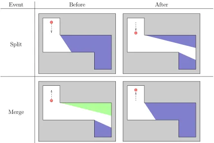
As the pursuers move, the shadows can change in any of ﬁve ways, called shadow

events.

• Appear: A new shadow can appear, when a previously visible part of the

envi-ronment becomes hidden.

• Disappear: An existing shadow can disappear, when one or more pursuers move

to locations from which that region is visible.

• Split: A shadow can split into multiple shadows, when the pursuers move in

such a way that a given shadow is no longer path-connected.

• Merge: Multiple existing shadows can merge into a single shadow, when

previ-ously disconnected shadows become path-connected.

• Push: An existing shadow can be pushed between pairs of neighboring

environ-ment reﬂex vertices, when the pursuer’s motion changes the cardinality of the

set of visible environment reﬂex vertices.

These events were originally enumerated in the context of the single-pursuer version

of this problem [27] and examined more generally by Yu and LaValle [96].

2.2.1 Shadow Labels

For our pursuit-evasion problem, the crucial piece of information about each shadow

is whether or not the evader might be hiding within it.

Definition 13. A shadow s is called cleared at time t if, based on the pursuers’

motions up to time t, it is not possible for the evader to be within s without having

(36)

Definition 14. A shadow is called contaminated if it is not clear. That is, a

con-taminated shadow is one in which the evader may be hiding.

We can assign a binary label to each shadow corresponding to the cleared/contaminated

status of the shadow. A label of 0 means that the shadow is cleared and similarly

a label of 1 means that the shadow is contaminated. Notice that, since the evader

can move arbitrarily quickly, the pursuers cannot draw any more detailed

conclu-sion about each shadow than its clear/contaminated status; if any part of a shadow

might contain the evader, then the entire shadow is contaminated. Using this

worst-case reasoning, we can completely represent the I-state given the pursuers’ current

conﬁguration and the current shadow labels.

Comparison Operators: Equal (=) and Not Equal (6=)

This section describes two comparison operators for shadow labels that test for

equal-ity. Consider two shadow labelsS = (s1s2. . . sk) and S

′ ₌

s′ 1s

′ 2. . . s

′

k

.

Definition 15. Two shadow labels S and S′ _are

equal to(=) one another if the

following holds:

∀i 1≤i≤k : si =s

′

i.

The intuition behind the (=) relation is that if a shadow appears as cleared in S

then it must also be cleared in S′_{. Similarly, if a shadow is contaminated in}

S then

it must also be contaminated inS′_.

Definition 16. Two shadow labels S and S′ _are

not equal to one another if the

following holds:

∃i 1≤i≤k : si 6=s

′

(37)

The intuition behind the (6=) relation is that there must exist at least one shadow

whose label is dissimilar between S and S′

. The not equal relation is the logical

negation of the equal to relation.

Binary Relation: Dominates (≫)

This sections describes a dominance binary relation over shadow labels. Consider two

shadow labelsS = (s1s2. . . sk) andS ′

= s′

1s ′ 2. . . s

′

k

.

Definition 17. A shadow labelSdominates a shadow labelS′ _{if the following holds:}

∀i 1≤i≤k : si ≤s

′

i.

Informally, S dominates S′ _{if for every shadow that is cleared in}

S′_{, the} correspond-ing shadow in S is also cleared. The intuition is that S provides at least as much

information as S′

, and can potentially contain more information in the case where

si = 0 and s

′

i = 1.

Definition 18. A shadow label S strictly dominates (≫) a shadow label S′

if

S ≫S′

and S 6=S′

. (2.3)

2.2.2 Label Update Rules

Each time a shadow event occurs, the labels can be updated based on worst case

reasoning. Below we describe the update rules for a shadow’s label according to the

visibility event that has occurred. Each rule describes how a label preceding the

visibility event is updated immediately following a given visibility event.

• Appear: New shadows are formed from regions that had just been visible, so

(38)

Event Before After

Appear

Disappear

Figure 2.2: An appear event increases the number of shadows by one, and the new shadow is labelled clear (green region). A disappear event decreases the number of shadows, its label is discarded.

• Disappear: When a shadow disappears, its label is discarded.

• Split: When a shadow splits, the new shadows inherit the same label as the

original.

• Merge: When shadows merge, the new shadow is assigned the worst label of

any of the original shadows’ labels. That is, a shadow formed by a merge event

is labeled clear if and only if all of the original shadows were also clear.

• Push: When a shadow is pushed, it maintains its current label.

Figures 2.2, 2.3, and 2.4 illustrate the shadow label update rules where cleared

shad-ows are represented as the ﬁlled path-connected green regions and contaminated

(39)

Event Before After

Split

Merge

Figure 2.3: When a shadow splits into multiple shadows, they inherit the same label as the original shadow. When a merge event occurs the new shadow is clear if and only if all of the original shadows are also clear.

2.3 Reformulating the Objective

We can incorporate this idea of reasoning about evaders via shadows to reformulate

the pursuer’s goal in terms of shadows rather than evader positions. Recall the

deﬁnition ofsolution strategyfrom Deﬁnition 10 where the pursuers’ goal was stated as

computing a ﬁnite time of capture for each evader over all possible evader trajectories.

Using the deﬁnitions of cleared and contaminated from above to describe a shadow’s

current status, we know that in the event that all of the shadows in the shadow region

are cleared, then we can be certain the evader has been seen at some point. The result

of this reasoning is that we can connect the shadow labels to our goal of ﬁnding a

solution strategy.

(40)

Event Before After

Push

Figure 2.4: A push event occurs when a shadow gets pushed between neighboring pairs of environment reﬂex vertices.

reaches a pursuer conﬁguration in ﬁnite time in which all of the shadows are cleared.

(41)

Chapter 3 Related Work

Pursuit-evasion problems are often classiﬁed under the vast umbrella of target

track-ing, security, and monitoring and surveillance problems. For brevity, this thesis will

use the term target tracking to refer to this collection of similar problems. Target

tracking problems typically require the system to ascertain some information about

a target (environmental feature and/or a mobile agent). Target tracking problems

span multiple disciplines and can be found in game theory [70,78], computational

ge-ometry [12,15,16,53], wireless networks [14,25,28], and mobile robotics [4,33]. In this

chapter we provide a brief overview of the target tracking problem (Section 3.1)

fol-lowed by a more focused literature review of Pursuit-Evasion problems (Section 3.2).

3.1 Target Tracking

As mentioned above, target tracking is a problem that spans multiple disciplines.

This thesis focuses on those works most closely related to mobile robotics. In the

most general case the objective for these problems is to maintain visibility between

the target and the tracker. Algorithms are known for planning the tracker’s motions

using dynamic programming [48], sampling-based methods [57], Partially Observable

Markov Decision Process (POMDP) [30], and reactive approaches [55]. The target

tracking task can be further complicated by additional constraints such as avoiding

detection [4], maintaining the target’s privacy [60], and bounded observer speed [54].

(42)

The ﬁrst problem is wireless sensor network assisted target tracking (Section 3.1.1)

and the second problem is monitoring and surveillance (Section 3.1.2). This is a small

sample of the various tasks and approaches encompassed within target tracking.

3.1.1 Wireless Sensor Network Target Tracking

As mentioned above, wireless sensor networks (WSNs), have been one approach used

to track a moving target(s). This target could be a human [14, 80], a moving vehicle

[26, 28, 97], or other moving target [3, 40, 79]. WSNs have been used in conjunction

with mobile robots [33, 62] to tackle the target tracking problem. Typically, the

mobile robots are used during sensor deployment with the goal of achieving good

sensor coverage [5,6]. However, their has been work done that focuses on the tracking

application after the deployment has occurred [63].

3.1.2 Monitoring and Surveillance

Monitoring and surveillance are two terms that are often used interchangeably. The

key distinction is that monitoring is a passive task that does not result in any direct

action on the agent’s part. The monitoring task typically charges the agent with

using its sensory information to detect a change in its environment. Surveillance

tasks are often seen as the active version of the monitoring problem where an agent

is tasked with actively searching its environment in an eﬀort to detect some change

in the environment.

Persistent monitoring and surveillance tasks are variations on the traditional

moni-toring and surveillance tasks that require a tracker or team of trackers to perform their

monitoring/surveillance task in perpetuity. The “perpetuity” aspect is what makes

these problems well-suited to be carried out by a robot or robot team.

Visibility-based monitoring problems commonly occur in many applications such as security and

(43)

The increased availability of mobile robots capable of performing these tasks has led

to increased interest [45, 51, 82] in recent years.

3.2 Pursuit-Evasion

This section examines existing literature in the ﬁeld of pursuit-evasion. Although

this thesis presents results for a visibility-based pursuit-evasion problem, we discuss

the evolution of the pursuit-evasion problem from diﬀerential games (Section 3.2.1)

to a graph-based formulation (Section 3.2.2) and ﬁnally to a geometric formulation

(Section 3.2.3).

3.2.1 Differential Games

The pursuit-evasion problem was originally posed in the context of diﬀerential games

[29,31] and has produced a variety of diﬀerent problems with small variations. In the

lion and man game, a lion tries to capture a man who is trying to escape [37, 58, 59,

77, 93]. In game theory, the homicidal chauﬀeur is a pursuit evasion problem which

pits a slowly moving but highly maneuverable runner against the driver of a vehicle,

which is faster but less maneuverable, who is attempting to run him over [31, 74].

Bounds for this problem that require the pursuer to physically capture the evader

suggests the number of pursuers required to satisfy this capture condition exceeds

that needed for the visibility-based pursuit-evasion problem [41].

3.2.2 Graph-Based Formulation

Pursuit-evasion on a graph can be traced back to the independent work done by

Parsons and Petrov. The motivation behind the Parsons’ problem was the desire for

a graphical model to represent the problem of ﬁnding an explorer who is lost in a

(44)

known as the edge-searching problem, is to determine a sequence of moves for the

pursuers that can detect all intruders in a graph using the least number of robots. A

move consists of either placing or removing a robot on a vertex, or sliding it along

an edge. A vertex is considered guarded as long as it has at least one robot on it,

and any intruder located therein or attempting to pass through will be detected. A

sliding move detects any intruder on an edge.

The Parsons’ problem and some of its results were later independently rediscovered

by Petrov [68] using slightly diﬀerent motivating problems. Petrov’s formulation

considered the cossacks and the robber game [69] and the princess and the monster

problem [31]. Golovach showed that both problems considered an equivalent discrete

game on graphs [23].

There are variations of graph-based pursuit-evasion that consider both edge

guard-ing and node guardguard-ing. One such formulation that diﬀers from edge-searchguard-ing (where

searchers move across edges and guard vertices) that has a direct application to

Robotics is the Graph-Clear problem [44]. Graph-Clear is a pursuit-evasion problem

on graphs that models the detection of intruders in an environment by robot teams

with limited sensing capabilities.

This is but a small sample of the existing literature surrounding the graph-based

pursuit-evasion problem. We have placed an emphasis on the inception of the problem

and brieﬂy touched on some recent results. For a more comprehensive review of

recent results in graph-based pursuit-evasion we direct the reader to the following

surveys [1, 9, 10, 21, 89].

3.2.3 Geometric Formulation

The visibility-based pursuit-evasion problem and the surveillance/tracking problem

are various types of pursuit-evasion problems that use a geometric formulation.

(45)

Yamashita [88] as an extension of the watchman route problem1 _{[16] and is a geometric}

formulation of the traditional graph-based pursuit-evasion problem. Research on the

visibility-based pursuit-evasion has produced numerous results for both the single

pursuer and multiple pursuer variants of the problem.

Single Pursuer Visibility-Based Pursuit-Evasion

There are many interesting results for the single pursuer visibility-based

pursuit-evasion problem. A complete solution [27], a randomized solution [32], and an optimal

shortest path solution have been found.

The capture condition for the general visibility-based pursuit-evasion problem

is deﬁned as having an evader lie within the pursuer’s capture region. There has

been substantial research focused how the visibility-based pursuit-evasion problem

changes when a robot has different capture regions. Thek-searcher is a pursuer with k visibility beams [50, 88], the∞-searcher is a pursuer with omni-directional field of view [27,66], and theφ-searcher is a pursuer whose field-of-view [22] is limited to an

angleφ∈(0,2π]. Note that all of these approaches consider evaders with unbounded speed.

Others have studied scenarios where there are additional constraints, such as the

case of curved environments [49], an unknown environment [75], a maximum bounded

speed for the pursuer [92], or constraints on the pursuer similar to those of a typical

bug2 _{algorithm [73].}

1

The objective of the watchman route problem is to compute the shortest path that a guard should take to patrol an entire area populated with obstacles, given only a map of the area.

2

(46)

Multiple Pursuer Visibility-Based Pursuit-Evasion

As a result of the problem complexity, there is a wide range of literature with diﬀering

techniques attempting to solve the multi-robot visibility-based pursuit-evasion

prob-lem. Some recent results involve using some of the pursuers as stationary sentinels

while other pursuers continue with the search [43]. Another approach involves

main-taining complete coverage of the frontier [20]. There are other variants of the

(47)

Chapter 4 GL

3 M Algorithm

The prior work of Guibas, Latombe, LaValle, Lin, and Motwani is integral in

un-derstanding some of the techniques that contribute to the results in this thesis. As

such, it is necessary to summarize the work of Guibas, Latombe, LaValle, Lin, and

Motwani [27] that presents a complete solution to the visibility-based pursuit-evasion

problem that utilizes a single pursuer.

4.1 Overview

The authors’ main contribution is a way to change the continuous problem of ﬁnding

a pursuer trajectory into a simpler discrete problem. Initially, the problem requires

a pursuer trajectory that solves the single pursuer visibility-based pursuit-evasion

problem. But by considering the areas of the environment that induce changes to

the shadow region we can ask the following equivalent question. What areas of the

environment does the pursuer have to visit to guarantee that the evader is captured?

Once a valid sequence has been found, returning a trajectory is trivial.

In the remainder of this chapter we investigate how certain pursuer motions can

force a critical information change within the shadow region (Section 4.2), and

de-scribe a graph structure and algorithm for solving the single pursuer visibility-based

(48)

Boundary

p

Contaminated Shadow

Path does not cross a critical boundary

p

Cleared shadow

Path crosses a critical boundary

Figure 4.1: An illustration of the concept of conservative regions.

4.2 Critical Information Changes

During the execution of a strategy, the pursuer must identify the contaminated

shad-ows in the shadow region. This piece of information is dependent upon the initial

position of the pursuer and the pursuer’s history of past positions, up to the current

time. As the pursuer moves, this information changes continuously; however, to

de-velop a complete algorithm, the authors need only be interested in tracking times in

which the pursuer’s information changes combinatorially. That is, we are only

con-cerned with pursuer movements that generate shadow events, as seen in Figure 4.1.

Definition 20. A region R ⊆ Wn _{is a} _{conservative region} _{if any path that remains}

within R generates no shadow events.

By deﬁnition a conservative region has the following information-conservative

prop-erty: while the pursuer remains within a conservative region the pursuer’s shadow

labels will not change.

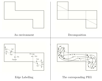
The original paper describes a visibility cell decomposition of the environment that

(49)

(a) (b) (c)

Figure 4.2: Ray shooting is performed for three general cases to form the conservative regions.

of the environment into conservative regions works by extending rays from inﬂection

points in the environment, and extending rays outwards from pairs of mutually visible

environment vertices. The inﬂection and bitangent ray extensions represent where

the pursuer’s shadow labels change.

There are ﬁve events that can occur at a critical event boundary that cause a

change in the pursuer’s shadow labels as it traverses between conservative regions.

These events (appear, disappear, split, merge, and push) were mentioned earlier in

Section 2.2.

The procedure used in creating the ray extensions provides the following

informa-tion about what type of event takes place along the boundary of the extension:

(a) Ray extensions caused by an inﬂection at a single endpoint of an environment

edge cause appear and disappear events.

(b) Ray extensions caused by a pair of mutually visible environment vertices (where

the vertices are not part of the same environment edge) cause split and merge

events.

(c) Ray extensions caused by inﬂections at both endpoints of an environment edge

cause push events.

(50)

An environment Decomposition Dis Dis Mer Spl Mer App Dis App App App Dis Spl 00 0 1 1 10 11 1 0 ₁ 0 00 0110₁₁ 00 0110₁₁ 01 0

Edge Labelling The corresponding PEG

Figure 4.3: An example of the Pursuit Evasion Graph for a given environment.

4.3 The Pursuit-Evasion Graph

With this information, the complete Pursuit-Evasion Graph (PEG) can be

con-structed as shown in Figure 4.3. The PEG is a directed graph composed of nodes

that contain a shadow labeling and a reference to a conservative region, where a node

exists for each possible shadow label combination for every conservative region. Its

edges are the set of critical events that occur from crossing an event boundary from

one conservative region to another. The algorithm starts at the PEG-node that

con-tainsp(0) with a shadow label of 1· · ·1. Using this node as the root of a graph search, the algorithm uses breadth-ﬁrst search to ﬁnd a path to a node with a shadow label

(51)

(52)

Chapter 5 An Optimal Strategy for a Single Pursuer

The speciﬁc problem we consider in this chapter is a variation on the visibility-based

pursuit-evasion problem in which a single pursuer moving through a simply-connected

polygonal environment seeks to locate an unknown number of evaders, each of which

may move arbitrarily fast. The pursuer has an omni-directional ﬁeld-of-view that

extends to the environment boundary.

The goal is to compute a pursuer strategy such that all evaders in the environment

lie within the pursuer’s ﬁeld-of-view at some ﬁnite time as the pursuer carries out

its search strategy, or to identify when no such strategy exists. Guibas, Latombe,

LaValle, Lin, and Motwani presented a complete algorithm for this problem [27], the

details of which appear in Chapter 4. However, the authors consider only feasibility

and do not attempt to compute optimal strategies. We build upon this work by

developing an algorithm that solves the visibility-based pursuit-evasion problem by

returning a solution strategy that is optimal in the sense that it minimizes the distance

travelled by the pursuer.

We use the same decomposition and Pursuit-Evasion Graph (PEG) discussed in

Section 4.2 and Section 4.3, but our algorithm must simultaneously consider multiple

paths to each node. Each of these paths can be viewed as a tour that travels through

an ordered sequence of cell boundaries. We introduce a pruning operation to

elimi-nate suboptimal paths, and a forward search algorithm whose termination condition

guarantees that an optimal solution will be found.

Measuring Strategic Communications

University of South Carolina

Scholar Commons

Visibility-Based Pursuit-Evasion In The Plane

Nicholas Michael Stiffler

Dedication

Acknowledgments

Abstract

Table of Contents

List of Tables

List of Figures

Chapter 1

Introduction

1.1

Motion Planning

1.1.1

Basic Ingredients of Planning

q

q

C

C

C

C

1.1.2

Properties of Planners

1.2

Thesis Organization

1.2.1

Single Pursuer - Shortest Path

1.2.2

Multiple Pursuers - Complete Solution

1.2.3

Multiple Pursuers - Probabilistically Complete

Sampling-Based Solution

1.2.4

Single Pursuer - Fixed Beams

Chapter 2

Problem Statement

2.1

Representing the environment, evaders, and

pursuers

2.2

Shadows

2.2.1

Shadow Labels

2.2.2

Label Update Rules

2.3

Reformulating the Objective

Chapter 3

Related Work

3.1

Target Tracking

3.1.1

Wireless Sensor Network Target Tracking

3.1.2

Monitoring and Surveillance

3.2

Pursuit-Evasion

3.2.1

Differential Games

3.2.2

Graph-Based Formulation

3.2.3

Geometric Formulation

Chapter 4

GL

3

M Algorithm

4.1

Overview

4.2

Critical Information Changes

4.3

The Pursuit-Evasion Graph

Chapter 5

An Optimal Strategy for a Single Pursuer