Statistical Stability and Spatial Instability in
Mapping Forest Tree Species by Comparing 9 Years of
Satellite Image Time Series
Nicolas Karasiak1,∗ , Jean-François Dejoux2 , Mathieu Fauvel2 , Jérôme Willm1, Claude Monteil1 and David Sheeren1 *
1 DYNAFOR, Université de Toulouse, INRA, Castanet-Tolosan, France
2 CESBIO, Université de Toulouse, CNES/CNRS/INRA/IRD/UPS, Toulouse, France
* Correspondence: [email protected]
Abstract: Mapping forest composition using multiseasonal optical time series is still challenging. Highly contrasted results are reported from one study to another suggesting that drivers of classification errors are still under-explored. We evaluated the performances of single-year Formosat-2 time series to discriminate tree species in temperate forests in France and investigated how predictions vary statistically and spatially across multiple years. Our objective was to better estimate the impact of spatial autocorrelation in the validation data on measurement accuracy and to understand which drivers in the time series are responsible for classification errors. The experiments were based on ten Formosat-2 image time series irregularly acquired during the seasonal vegetation cycle from 2006 to 2014. Due to lot of clouds in the year 2006, an alternative 2006 time series using only cloud-free images has been added. Thirteen tree species were classified in each single-year dataset based on the SVM algorithm. The performances were assessed using a spatial leave-one-out cross validation (SLOO-CV) strategy, thereby guaranteeing full independence of the validation samples, and compared with standard non-spatial leave-one-out cross-validation (LOO-CV). The results show relatively close statistical performances from one year to the next despite the differences between the annual time series. Good agreements between years were observed in monospecific tree plantations of broadleaf species versus high disparity in other forests composed of different species. A strong positive bias in the accuracy assessment (up to 0.4 of Overall Accuracy) was also found when spatial dependence in the validation data was not removed. Using the SLOO-CV approach, the average OA values per year ranged from 0.48 for 2006 to 0.60 for 2013, which satisfactorily represents the spatial instability of species prediction between years.
Keywords: tree species, forest, biodiversity, time series, spatial autocorrelation, cross-validation, accuracy.
1. Introduction
Forest ecosystems play a major role in global biodiversity [1]. They provide several services to humanity including carbon sequestration (which regulates climate [2]), timber production[3], soil protection[4], and recreation. They also have an impact on human health and well-being. However, the provision of such ecosystem services depends on several factors including the diversity of tree species [5]. Therefore, knowing the distribution of tree species in forests is crucial to assess ecosystem functions and services. More broadly, information on tree species is required for forest management and also for long-term forest monitoring, especially in the current context of climate change and related disturbances (forest fires, windstorms, drought, pests and diseases) [6].
Remote sensing has long been used to collect information on forest resources including stand composition [7,8]. Nevertheless, accurately distinguishing tree species is still challenging [9]. In the past, maps of tree species were based on field surveys completed by computer-aided analysis of aerial
photographs [10,11]. While this approach provides accurate operational results for forest managers, it is limited to small spatial extent because it is costly and time consuming, which also affects its updating. In the last few decades, various types of remotely sensed images have been used to automate the identification of forest tree species. Some authors focused on the spatial resolution using very high-resolution satellite or airborne imagery [12–15]. They assumed the classification would benefit from the spatially detailed information and would therefore be accurate. Despite some successful results, this approach revealed itself to be of limited interest when only a single date was used due to the low spectral resolution of the data because of the reduced spectral and temporal information. Alternatively, as tree morphology and biochemical traits have a subtle influence on spectral reflectance [16], several authors explored airborne hyperspectral imagery [17–19]. Depending on the number of classes of species, on the methodology used for classification, and on the characteristics of the images (pixel size, number of spectral bands), the accuracy of the classification varied. Nevertheless, studies based on hyperspectral imagery were typically more accurate than those based on single-date multispectral data [9].
Taking advantage of the temporal dimension of the satellite data was another way to separate tree species [9]. Time series can capture the phenological behavior of the vegetation and this functional trait can be useful to discriminate the forest types. Changes in pigment contents, water and leaf morphology across seasons can vary from one species to another. Time series with images covering all phenological events from green-up to senescence (leaf-on, spring flush, autumn senescence, leaf-off) can produce detailed classification results. The use of multitemporal data for this purpose is not new. This approach has been explored from various image datasets of different spatial and temporal resolutions based on spaceborne sensors such as MODIS [20,21], Landsat [22–26], RapidEye [27], as well as airborne sensor [28,29] or unmanned aerial systems [30]. More recently, the potentialities of the new freely available high spatial resolution Sentinel-2 (S2) data have been investigated [31–35]. In general, authors found a benefit to combine images acquired in spring and autumn, at the key phenological stages of temperate forests since it influences positively the classification accuracy. Summer images are also frequently selected in features ranking procedure, especially for conifer species [35] but also for deciduous tree species [29]. From a spectral point of view, red-edge bands and SWIR bands were reported as important variables when S2 time series were used [31–33].
More recently, the potential of the new freely available high spatial resolution Sentinel-2 (S2) data has been investigated [31–35]. In general, the authors found it advantageous to combine images acquired in spring and autumn, at the key phenological stages of temperate forests, since it had a positive influence on the accuracy of the classification. Images acquired in summer are also frequently selected in features ranking procedures, particularly for conifer species [35], but also for deciduous species [29]. From a spectral point of view, red-edge bands and SWIR bands are reported to be important variables when S2 time series are used [31–33].
Despite the increasing number of studies that use time series to identify forest types, the true predictive power of these kinds of data remain to be demonstrated. Even though it is difficult to compare studies because of the use of different methods, sensors, and classes of tree species, we observed very contrasted results from one study to another. For instance, using four dates for S2 data in 2017, Perssonet al.[33] obtained a kappa value of 0.83 to classify five species (Norway spruce, Scots pine, Hybrid larch, Birch and Pedunculate Oak). This differs substantially from the Immitzer’s results [31] who observed a kappa of 0.59 to identify seven species including Norway spruce, Scots pine, European larch and Oak species based on two S2 images.
that affect the classification of species, as recommended by [9]. Several drivers of classification errors remain insufficiently explored, among which, spatial autocorrelation of reference data has long been identified but rarely quantified [38,39]. Spatial dependence in the reference data due to an inadequate sampling strategy to split training and validation sets can wrongly increase classification accuracy [38,40,41]. Contamination by clouds and cloud shadows in dense image high resolution time series may also have a major impact on classification. Because the distribution of such contamination may vary over time and in space across years, a multiyear analysis is required to reliably evaluate their effect.
To our knowledge, this is the first study of variability between one-year classifications of tree species based on multiple years using dense image high spatial resolution time series. We evaluated the classification performance of single-year Formosat-2 time series in distinguishing forest types with spatially independent validation data. We also investigated how the predictions vary statistically and spatially across multiple years (from 2006 to 2014). The main contribution of this work is a better estimation of the classification accuracy of the forest maps by reducing optimistic bias due to spatial autocorrelation. The second contribution, resulting from the first, is a finer understanding of the drivers responsible for classification errors. We hypothesize that time series data improve species discrimination compared to single-date image due to seasonal variability in spectral reflectance between species. We also hypothesize that spatial autocorrelation between training and validating sets will bias the statistical performances positively due to the non-independence of the reference samples.
2. Material
2.1. Study area
The study site is located in south-western France, next to Toulouse, and covers an area of 24 km x 24 km (Fig1). This delimited area was determined by a satellite acquisitions scheme by theCentre National d’Etudes Spatiales(CNES) who acquired a Formosat-2 Satellite Image Time Series (SITS) of the site. The Garonne river crosses the eastern part of the study area, influencing soil composition and the nearly flat topography of the area. The climate is sub-Atlantic characterized by sunny autumns, hot dry summers, and mild rainy winters (the average annual temperature is >13◦C; annual precipitation = 656 mm). The landscape is dominated by arable lands (including wheat, sunflower, maize) and grasslands. Forests cover up to 10% of the landscape (53 km2).
2.2. Satellite image time series
We used a dense optical image dataset composed of Formosat-2 time series acquired in nine consecutive years from 2006 to 2014. This dataset was obtained during preparation for the Sentinel-2 and VENµS mission with cooperation between the Israeli Space Agency (ISA) and the French CNES
[42]. A total of 156 dates was acquired with an average of 14 images per year and a maximum of 43 images in 2006. The distribution of the dates over time varied from one year to another and the number of images available during the growth season differed from the number available at the end of vegetation season (Figure2).
Cloud coverage also varied considerably from one date to another, ranging from a minimum of 8 cloud-free images in 2011 to a maximum of 20 in 2006. For 2006, by visual inspection, we created an additional dataset (named 2006 bis) by selecting only the cloud-free images, resulting in a time series of 20 dates (compared to the original 46).
The Formosat-2 multispectral images are delivered in an 8-bit radiometric resolution. Each image provides 4 spectral bands ranging from the visible (Blue: 0.45–0.52µm, Green: 0.53–0.60µm, Red:
0.63–0.69µm) to the near-infrared (NIR: 0.76–0.90µm) with a nominal pixel size of 8 m. All the images
were acquired under a constant viewing angle and a field of view of 24 km like Landsat, VENµS and
2.3. Ancillary data
A forest mask produced in 1996 by the French National Forest Inventory database (IGN BDForêt®, v.1) was used to select forest pixels in the SITS (i.e. forest stands with a minimum area of 2.25 hectares) and to exclude non-forested areas. Based on aerial photographs taken in 2006, 2010 and 2013 (IGN BDOrtho®), the mask was manually updated to retain only SITS forest stands that remained stable over the nine year period
2.4. Field data
Four field campaigns were conducted between November 2013 and January 2017 to identify and locate reference samples of tree species in the study site. All the main forests were visited. Only the dominant broadleaf and conifer tree species were recorded. To insure tree species purity in the training samples, plots were delimited at the center of homogeneous areas covering an area of approximatly 576 m2(i.e. nine contiguous 8 m × 8 m Formosat-2 pixels). Only the pixel at the center of each area was used for the classification protocol. Plots were located using a Garmin GPSMap 62st receiver (3-5 m accuracy) and distributed over 72 distinct forest stands.
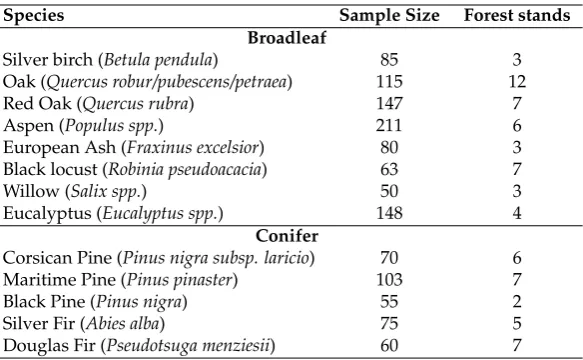
Thirteen tree species of which eight were broadleaf species and five conifer species were studied (Table1). In some species, identification was limited to the genus level because of the existence of cultivars (case of Aspen) and the difficulty involved in determining the exact species in some cases Oak, Willow and Eucalyptus. We acquired a total of 1262 sample plots. Class distribution was moderately imbalanced reflecting the uneven distribution of species abundances in the forests. The number of samples varied from 50 (the minimum for Willow) to 211 (the maximum for Aspen). Conifers were less well represented with an average of 73 samples per class compared with 112 for broadleaf species.
3. Classification protocol
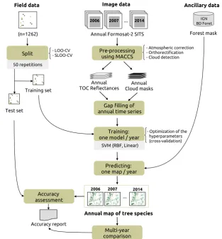
A global overview of the classification protocol applied on each Formosat-2 single-year time series is shown in Figure3.
TOULOUSE
PARIS
43
°3
0ʹ
0ʺ
N
43
°2
4ʹ
0ʺ
N
1°0ʹ0ʺE 1°6ʹ0ʺE 1°12ʹ0ʺE 1°18ʹ0ʺE 1°24ʹ0ʺE
Jan. Feb. Mar. Apr. May. Jun. Jul. Aug. Sep. Oct. Nov. Dec.
2006
43 dates
2006bis
20 dates
2007
15 dates
2008
11 dates
2009
16 dates
2010
14 dates
2011
12 dates
2012
13 dates
2013
17 dates
2014
15 dates
Figure 2.Number and acquisition dates of each image in the Formosat-2 time series from 2006 to 2014.
Table 1.List of tree species with their sample size, in pixels, collected during field surveys (n=1262). The number of forest stands in which the samples were collected is also provided. Stand delimitation is based on the French National Forest Inventory database (IGN BDForêt®v.1)
Species Sample Size Forest stands
Broadleaf
Silver birch (Betula pendula) 85 3
Oak (Quercus robur/pubescens/petraea) 115 12
Red Oak (Quercus rubra) 147 7
Aspen (Populus spp.) 211 6
European Ash (Fraxinus excelsior) 80 3
Black locust (Robinia pseudoacacia) 63 7
Willow (Salix spp.) 50 3
Eucalyptus (Eucalyptus spp.) 148 4
Conifer
Corsican Pine (Pinus nigra subsp. laricio) 70 6
Maritime Pine (Pinus pinaster) 103 7
Black Pine (Pinus nigra) 55 2
Silver Fir (Abies alba) 75 5
Douglas Fir (Pseudotsuga menziesii) 60 7
3.1. Pre-processing
Field data Ancillary data
Forest mask
Pre-processing using MACCS
Training set
Test set (n=1262)
- Atmospheric correction - Orthorectification - Cloud detection
- Optimization of the hyperparameters (cross-validation)
IGN BD Foret
Split
Image data
2007 ... 2014
Annual Formosat-2 SITS
Annual Cloud masks Annual
TOC Reflectances
Gap filling of annual time series
Training: one model / year
SVM (RBF, Linear)
Predicting: one map / year
Accuracy assessment
Accuracy report
2014 ...
Annual map of tree species
Multi-year comparison 2006
2006
2007
- LOO-CV - SLOO-CV
50 repetitions
Figure 3.Classification protocol for a single year time series, repeated for the 9 years available from 2006 to 2014. The splitting procedure to create independent training and test sets is based on a spatial and non-spatial leave-one-out cross-validation (SLOO-CV and LOO-CV respectively). The LOO-CV were trained with exactly the same number of training samples as the SLOO-CV, after random undersampling.
cloud is likely to be present. Based on this method, masks of clouds and related shadows are produced by MACCS for each image in the time series.
In the second step, SITS of each year were filtered using a linear gap-filling algorithm applied to each spectral band to remove noisy data (i.e. cloudy and shady pixels) and to retrieve their surface reflectance [46]. Invalid pixels were replaced by the interpolated values from the closest available valid pixels in the time series. Gap-filling was chosen for its simplicity and its previously demonstrated efficiency already demonstrated when time gaps between consecutive images are limited [47].
3.2. Training
Classification models were built for each year with exactly the same pixels for training and testing using the supervised SVM (Support Vector Machine) classifier [48] known to be the best approach in the case of small training data sets with respect to data dimensionality [49]. In this study, we selected the Radial Basis Function (RBF) kernel which is the most frequently used and has already been proven to be effective in the case of similar classification problems [50]. Hyperparameters including the regularization parameter (C) and the kernel bandwidth (γ) were tuned by cross-validation in a search
space with the following settings :C={0.01, 0.1, ..., 110} andγ={1−9, 1−8, ..., 13}. A linear kernel was
proportional to class frequencies. SVM was computed using the scikit-learn python library [52]. Vector of features were standardized (i.e. centering and scaling to unit variance) prior to training.
3.3. Estimating prediction errors by spatial cross-validation
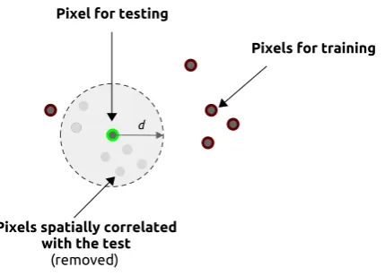
Because spatial autocorrelation between reference samples may produce optimistic bias in assessments of classification performance [38,40,41], we used a spatial leave-one-out cross-validation (SLOO-CV) sampling strategy [53,54] to separate the training and test sets to guarantee full independence between them. In this approach, one reference sample is used as the test set and the remaining samples, non-spatially correlated with the test set, are used as the training set (Figure4). This is repeatedntimes wherenequals the number of reference samples. Thenprediction results are then averaged to obtain an estimation of the prediction error. In our case, the test set was composed of one pixel of each class (i.e. a total of 13 pixels at each iteration) and the procedure was repeated 50 times, this being the number of reference samples of the lowest class size. We compared this splitting procedure with the classical non-spatial leave-one-out cross-validation strategy (LOO-CV) using the same training size per class as in SLOO-CV, by random undersampling. For year-to-year comparison, we also used the same training and test sets related to each sampling approach by setting the same random seed.
d Pixel for testing
Pixels for training
Pixels spatially correlated with the test
(removed)
Figure 4.Spatial leave-one-out cross-validation (SLOO-CV) schema for one class. One pixel is used for testing. The other pixels are used for training, except pixels geographically too close to the pixel selected for testing. This procedure is repeatedntimes wherenis the number of reference samples. Spatial autocorrelation between nearby pixels is assumed up to a distancedwhich can be estimated using Moran’s I.
The spatial autocorrelation distance was estimated by computing the Moran’s Index from the pixels of forests in the SITS [55]. Moran’s I estimates the correlation between the value of a variable at one location and nearby observations. The index ranges from -1 (negative spatial autocorrelation) to +1 (positive spatial autocorrelation) with a value close to 0 in the absence of spatial autocorrelation (random spatial distribution). More formally, the Moran’s I is defined as the ratio of the covariance between neighborhood pixels and the variance of the entire image:
I(d) = n
S0 n
∑
i=1 n
∑
j=1
wi,j(xi−x)(xj−x) n
∑
i=1
(xi−x)2
(1)
S0= n
∑
i=1 n
∑
j=1
wi,j (2)
In this study, Moran’s I was computed for each spectral band of each year, for neighborhoods (lags) varying from 1 to 100 pixels (i.e. from 8 m to 800 m). Based on correlograms, we evaluated the distance between nearby pixels for which Moran’s I equals 0.2, considering the potential effect of spatial autocorrelation as not significantly different from the thresold value of Moran’s I [56]. Then, the median distance was calculated for each spectral band, taking all the dates of one year into account (Figure5). This was done for each year. Finally, the average value of the median distance of each year was kept in the spatial cross-validation procedure to split the training and test sets. This average value was estimated to be 340 m (i.e. 42 pixels).
8m 88m 168m 248m 328m 408m 488m 568m 648m 728m 808m 0.0
0.1 0.2 0.3 0.4 0.5 0.6 0.7 0.8 0.9 1.0
Moran's i
528m
blue bands
8m 88m 168m 248m 328m 408m 488m 568m 648m 728m 808m
168m
green bands
8m 88m 168m 248m 328m 408m 488m 568m 648m 728m 808m
176m
red bands
8m 88m 168m 248m 328m 408m 488m 568m 648m 728m 808m
144m
near infrared bands
8m 88m 168m 248m 328m 408m 488m 568m 648m 728m 808m Lag (in meter)
176m
All bands in 2013
median
Figure 5. Moran’s I correlograms of each Formosat-2 spectral band of the SITS 2013, for pixels representing forests. Each curve represents one date of the SITS. the red dashed line represents the median distance value (in x) where Moran’s I = 0.2 (in y). For a Moran’s I thresold value of 0.2, spatial independence between nearby pixels was assumed. This is the case beyond to 528 m in the blue band, 168 m in the green, 176 m in the red and 144 m in the near-infrared.
3.4. Accuracy assessment of one-year classifications and comparison
The results of the classifications were assessed according to the confusion matrix based on Overall Accuracy (OA) and the F1 score (i.e. the harmonic mean of precision and recall varying from 0 for the worst case to 1 for perfect classification), errors of omission and errors of commission. A Wilcoxon signed-rank test was used to determine if the difference in accuracy between annual classifications and sampling strategies (LOO-CV vs SLOO-CV) was statistically significant.
4. Results
4.1. Overall statistical performances
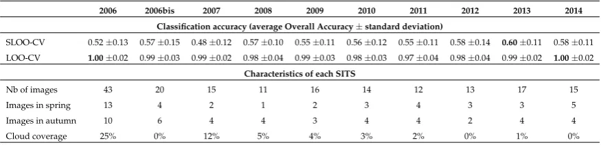
The classification performances for each year are presented in Table2. Generally speaking, the performances were similar between the years but very different between sampling strategies (SLOO-CV vs LOO-CV) in a given year.
When prediction errors were estimated by spatial cross-validation (SLOO-CV), the average OA varied from 0.48 in 2007 to 0.60 in 2013 with high variability in the results (average standard deviation of 0.12). No significant differences were observed between the years 2008-2012, 2012-2014 and between 2006 and 2007 which were the cloudiest SITS (p < 0.05; Wilcoxon signed-rank test statistic; see AppendixBfor statistical details). For the year 2006, when cloudy images were removed from the SITS (i.e. using the 2006bis dataset), the classification was improved, the performance was similar to that in the other years (average OA = 0.57). The best classification was obtained using the 2013 time series (average OA = 0.60).
When accuracy was computed using the standard leave-one-out cross-validation (LOO-CV), prediction errors were very low compared to when SLOO-CV was used, suggesting a high optimistic bias in the evaluation. The average OA varied from 0.97 in 2011 to 1.00 in 2006 and 2014 with a standard deviation close to zero. The cloudiest years (2006 and 2007) did not differ significantly in performance from the other years in most cases (AppendixB). These results contradict the previous ones: while the year 2007 was the worst with the SLOO-CV, with LOO-CV it had the second best score.
In the following sections, we only detail the results based on the SLOO-CV strategy since it best reflects the true performance of the classifications.
Table 2.Accuracy report of spatial leave-one-out cross-validation (SLOO-CV) sampling strategy and leave-one-out cross-validation (LOO-CV) for each single-year classification based on OA statistics. The 2006bis time series only includes cloud-free images of 2006. The average percentage of cloud coverage was estimated by computing for each species the number of time each reference sample was affected by clouds (detected from the MACCS processing chain).
2006 2006bis 2007 2008 2009 2010 2011 2012 2013 2014
Classification accuracy (average Overall Accuracy±standard deviation)
SLOO-CV 0.52±0.13 0.57±0.15 0.48±0.12 0.57±0.10 0.55±0.11 0.56±0.12 0.55±0.11 0.58±0.14 0.60±0.11 0.58±0.11 LOO-CV 1.00±0.02 0.99±0.03 0.99±0.02 0.98±0.04 0.99±0.03 0.98±0.03 0.97±0.04 0.98±0.04 0.99±0.02 1.00±0.02
Characteristics of each SITS
Nb of images 43 20 15 11 16 14 12 13 17 15
Images in spring 13 4 2 1 2 3 4 3 3 5
Images in autumn 10 6 4 4 3 4 4 2 4 4
Cloud coverage 25% 0% 12% 5% 4% 3% 2% 0% 1% 0%
4.2. Accuracy per species
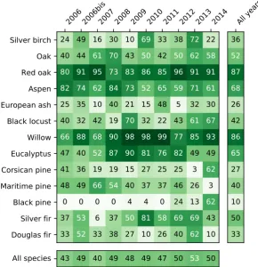
In most cases, whatever the year, broadleaf tree species were better discriminated than conifers (Figure6). The highest performances were obtained for monospecific plantations of Red oak (average F1 score = 87%), Aspen (average F1 score = 68%) and Willow (average F1 score = 86%). Aspen was also detected with good accuracy (average F1 score = 68%). Conversely, some species were difficult to identify, including European ash (average F1 score = 26%) and Silver birch (average F1 score = 36%) except in the years 2010 and 2013.
2006 2006bis2007 2008 2009 2010 2011 2012 2013 2014
Silver birch
Oak
Red oak
Aspen
European ash
Black locust
Willow
Eucalyptus
Corsican pine
Maritime pine
Black pine
Silver fir
Douglas fir
24 49 16 30 10
69
33 38
72
22
40 44
61 70
43
50
42
50 62 58
80 91 95 73 83 86 85 96 91 91
82 74 62 84 73 52 65 59 71 61
25 35 10 40 21 15 48 5 32 30
40 32 42 19
70
32 22 43
61 67
66 88 68 90 98 98 99 77 85 93
47 40
52 87 90 81 76 82
49 49
41 36 19 19 15 27 25 25 3
62
48 49
66 54
40 37 37 46 26 3
0 0 0 0 4 4 0 24 13
62
37
53
6 37
50 81 58 69 69
43
33
52
33 38 27 10 26 40
62
10
All years
36
52
87
68
26
42
86
65
27
40
10
50
33
All species 43 49 40 49 48 49 47 50
53
50
Figure 6.Average F1 score (in %) per species and per year based on the SLOO-CV sampling strategy using the SVM (RBF kernel) classifier. Values range from white (F1 score = 0%) to dark green (F1 score = 100%). Average values of F1 score per year and per species are also provided (in the bottom row and last column on the right, respectively).
On average, the year 2013 was the best, mainly because of a high score for Silver birch compared to the other years. Year 2007 was the least accurate. Higher performance disparity was observed from one year to another for most species, except Red oak and Willow.
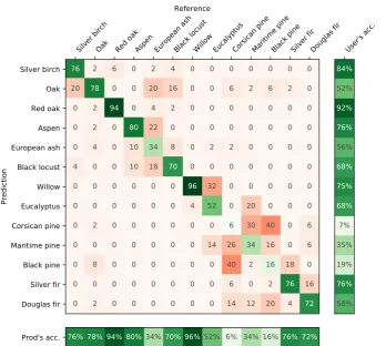
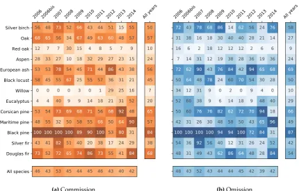
4.3. Confusion between species
Generally, when errors occurred, the broadleaf tree species were confused with each other as well as with conifers. The main source of omissions for Silver birch was mispredictions as Oak which, in turn, was confused with European ash but also with Black locust and with some pines (see the confusion matrix for the year 2013 in Figure7, for example). Red oak was the subject of very little confusion. High rates of omissions were observed for European ash with misclassifications as Oak, Aspen and Black locust. Under-detection was also observed for the evergreen Eucalyptus plantations due to confusion with Willow. In conifer species, the errors mainly appeared between species of Pine but also between Pine and Douglas fir.
Confusions between species were similar from one year to another but the commission and omission errors rates varied and accuracy was very low for some species (Figure8).
4.4. Spatial agreement between years
Silver birchOak Red oakAspen European ashBlack locustWillow EucalyptusCorsican pineMaritime pineBlack pineSilver firDouglas fir
Reference
Silver birch Oak Red oak Aspen European ash Black locust Willow Eucalyptus Corsican pine Maritime pine Black pine Silver fir Douglas fir
Prediction
76 2 6 0 2 4 0 0 0 0 0 0 0
20 78 0 0 20 16 0 0 6 2 6 2 0
0 2 94 0 4 2 0 0 0 0 0 0 0
0 2 0 80 22 0 0 0 0 0 0 0 0
0 4 0 10 34 8 0 2 2 0 0 0 0
4 0 0 10 18 70 0 0 0 0 0 0 0
0 0 0 0 0 0 96 32 0 0 0 0 0
0 0 0 0 0 0 4 52 0 20 0 0 0
0 2 0 0 0 0 0 0 6 30 40 0 6
0 0 0 0 0 0 0 14 26 34 16 0 6
0 8 0 0 0 0 0 0 40 2 16 18 0
0 0 0 0 0 0 0 0 6 0 2 76 16
0 2 0 0 0 0 0 0 14 12 20 4 72
User's acc.
84%
52%
92% 76%
56%
68% 75% 68%
7% 35% 19%
76%
58%
Prod's acc. 76% 78% 94% 80%34%70% 96%52% 6% 34% 16%76% 72%
Figure 7.Confusion matrix for 13 tree species for year 2013. Each cell provides an average value of agreement or confusion (in %) based on 50 classifications (number of iterations) using the SLOO-CV sampling strategy.
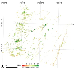
When spatial uncertainty was analyzed using the map of agreements between the one-year classifications, good stability was observed in the monospecific tree plantations of broadleaf species (Figure9). The stands composed of Aspen, Red oak, and Eucalyptus were clearly differentiated. In contrast, in complex forests including a mix of different species, disagreements between annual classifications were higher, as suggested by the previous statistical assessment. An example is given in Figure10showing a mix forest composed of conifers (mainly Black pine but also Douglas fir and Silver fir) and deciduous species (mainly Oak and Silver birch). There was considerable confusions between conifer species from one year to another (low agreement). The extent of Silver birch areas was also highly variable. In this forest, the dominant species were rather well-identified but their exact location was inaccurate at the pixel level.
Significant disagreements between the classifications were also observed in other contexts, especially in thin riparian forests and forest edges where species composition and diversity is high, with lots of species unsampled (Figure9). This was also true in low density forest stands, for which confusions appeared with the understory vegetation. Finally, disagreements were also observed in areas very affected by clouds and shadows.
5. Discussion
20062006bis2007 2008 2009 2010 2011 2012 2013 2014 Silver birch Oak Red oak Aspen European ash Black locust Willow Eucalyptus Corsican pine Maritime pine Black pine Silver fir Douglas fir
56 48 73 52 66 43 44 51 15 55
68 65 56 34 67 49 63 60 48 57 12 7 7 30 15 4 8 5 7 9 28 33 27 10 18 32 29 27 23 15 53 53 78 54 45 71 44 86 43 38 58 45 55 67 25 55 57 36 31 21 0 0 0 0 3 0 1 29 25 16 4 4 40 9 9 14 18 21 31 52 53 54 73 69 68 71 56 68 92 48 48 55 32 50 58 55 66 50 64 90 100 100 100 100 89 90 100 53 80 31 43 41 82 51 40 20 38 17 24 29
73 52 72 65 74 86 73 55 41 84 All years 50 57 10 24 56 45 7 20 65 57 84 38 68
All species 46 43 53 45 44 45 46 43 40 42
(a)Commission
20062006bis2007 2008 2009 2010 2011 2012 2013 2014 72 43 78 68 86 14 62 56 24 76
31 38 16 18 30 40 40 28 21 14 16 6 2 18 12 12 12 2 6 6 7 14 31 12 19 38 28 36 19 36
72 62 90 43 76 84 42 94 65 68
50 64 48 78 24 60 70 54 30 28 34 12 31 9 0 2 0 9 4 0 52 60 38 9 6 14 18 9 48 40 50 60 76 76 82 62 72 70 94 18 42 31 26 30 48 58 50 43 65 96 100 100 100 100 94 94 100 72 84 31 54 36 92 56 40 12 31 26 24 52 48 31 49 43 62 86 64 48 28 84
All years 58 27 9 24 69 50 10 29 66 49 87 42 54
48 43 52 43 44 44 45 42 39 42
(b)Omission
Figure 8.Average rate of commission and omission errors (in %) per species and per year based on the SLOO-CV sampling strategy.
present study is a first attempt to assess the robustness of tree species discrimination in multiple years and to better understand the drivers that affect classification performances.
5.1. Effect of spatial autocorrelation: the SLOO-CV strategy as a standard
Our results revealed a strong positive bias in validation based on the usual LOO-CV strategy for splitting reference data. This bias was already suspected in a previous study when we used stratified-k-fold but was not quantified [37]. Regarding the importance of the overestimation in the classification accuracy (∆OA>0.4 between LOO and SLOO-CV), the use of spatially independent data for validation should no longer be an option but wherever possible, a requirement, in agreement with the recommendation of [9].
Spatial autocorrelation in the reference data has long been known to affect the classification and accuracy assessment [38,39,57,58]. Different sampling strategies for data splitting have already been studied in the literature including spatial [41,54,59,60] and aspatial approaches [59,61–63]. Although the spatial sampling approach is recommended to reduce the spatial autocorrelation effect, an aspatial (i.e. random, systematic or stratified) sampling strategy assuming independence between samples is usually used in remote sensing analyses for the sake of simplicity [63].
43
°3
0ʹ
0ʺ
N
43
°2
4ʹ
0ʺ
N
1°0ʹ0ʺE 1°6ʹ0ʺE 1°12ʹ0ʺE 1°18ʹ0ʺE
1 2 3 4 5 6 7 8 9 10
number of agreements
1 3 5 6 8 10
Figure 9. Spatial comparison between the annual classifications of forest tree species from 2006 to 2014 (including 2006bis). The number of agreement is the modal value related to the class with the highest frequency. This map illustrates the stability of predictions from one year to another with a high number of disagreements in red (high uncertainty) and a low number of disagreements in green (high accuracy). In many cases, homogeneous green areas are tree plantations of broadleaf species such as Red Oak and Aspen or Eucalyptus.
An important point to note is that we guaranteed complete independence between the training and validation sets but not among the training samples. Thus, spatial autocorrelation still persisted in the training set. Compared to LOO-CV, the SLOO-CV strategy provides a statistical estimate of accuracy that fits the quality of the map product better (and hence predictive performance) but in terms of predictions, the results of classification results are similar. This is illustrated by the number of agreements between the annual classifications for both LOO-CV and SLOO-CV (Figure11). With the exception of some classes (e.g. Maritime and Black pine), the distribution of agreements per class of species is rather similar.
5.2. Effect of the size of the reference sample
presence of noise on the data (under detected clouds or cloud shadows under-detected, see below) may have a greater negative impact on their discrimination. However, Willow is an exception, as it was the least populated species with only 21 samples for training and a total of three forest stands but obtained the second highest F1 score (average = 0.86) behind Red oak (average = 0.87) with 118 samples (AppendixD)
More generally, due to the complexity of the learning problem (i.e. partial overlapping between spectro-temporal signatures of species in the feature space), increasing the size of the training sample and reducing the degree of imbalance in class distribution should improve the predictive performance [68]. In a recent study, Bolynet al.[32] obtained a high degree of accuracy (OA = 88.5%) when they classified 11 forest classes (including seven tree species) in the entire Belgian Ardenne ecoregion with only two Sentinel-2 dates. Although this statistical performance may be partially inflated by spatial autocorrelation, this greater accuracy could also be explained by the large sample size (from 2,589 to 7,068 pixels for each class with a minimum of 31 forest stands and a maximum of 64). An equivalent level of performance (OA = 88.2%) was obtained by [33] when they identified five tree species in a forest in central Sweden using four S2 images acquired from spring to autumn. However, in their case study, the sample size was very close to ours (from 27 to 98 pixels per species). Spatial overfitting is suspected, as in our previous work [37].
5.3. Effect of clouds and cloud shadows
When we compared the stability of predictions from one year to another (i.e. the map of agreements between the annual classifications) with the number of times the pixels were affected by clouds or cloud shadows, we found no significant correlation. This indicates that disagreements between the classifications can not be attributed to this factor. We observed that the years most affected by clouds (2006 and 2007) had the lowest average OA values (52% and 48% respectively, see Table
1km
1 3 5 6 8 10
BDOrtho IRC 2013 Number of agreements 2006 2006bis
2007 2008 2009 2010
2011 2012 2013 2014
Silver birch
Oak
Red oak Aspen European ash Black locust
Willow
Eucalyptus
Corsican pine Maritime pine Black pine
Silver fir
Douglas fir
Species 0
2 4 6 8 10
Number of agreement
(a)LOO-CV sampling
Silver birch
Oak
Red oak Aspen European ash Black locust
Willow
Eucalyptus
Corsican pine Maritime pine Black pine
Silver fir
Douglas fir
Species 0
2 4 6 8 10
Number of agreement
(b)SLOO-CV sampling
Figure 11.Distribution per species of the number of agreements between the annual classifications using all the predicted pixels for both the LOO-CV and SLOO-CV sampling strategies.
2). However, for the other years, the F1 score per species was not always consistent with the extent of cloud coverage. For instance, in 2008, 11% of the reference pixels for Oak were affected by clouds (AppendixC) but the F1 score was the highest of all the years. This suggests that when clouds and cloud shadows are detected by the MACCS processing chain, the gap-filling approach is appropriate to correct noisy pixels. This procedure is currently used in the French production center THEIA (https://theia.cnes.fr) for Landsat, VENµS and Sentinel-2 level2A products.
An in-depth visual analysis of the map products in fact revealed that this disturbance factor had a major effect on classification performances. When the forests were partially affected by clouds and cloud shadows or when these were under detected (which is what happened in the case of slight fog), spectral signatures were skewed and confusion between species was likely. This issue is illustrated in Figure12which shows changes in the reflectance values of an Oak pixel in 2006. On most of the dates, the pixel was free of clouds and shadows (green dots). In some cases, clouds or cloud shadows were found and the pixel values were gap-filled by linear interpolation (orange dots). But on certain dates, clouds or cloud shadows were not detected (red dots) and this influences the spectro-temporal signature. These dates had erroneous values but also had a negative impact on nearby gap-filled values since the dates are considered to be valid (e.g., see the 10th image in Figure12). Another example showing an erroneous spatial pattern in a forest stand due to undetected clouds is provided in AppendixC.3. This noise may influence the training step through the addition of inadequate support vectors, as well as the validation step, if the reference pixel to be tested is impacted by noise but the training pixels are not.
Feb Mar Apr May Jun
Jul
Aug Sep Oct Nov Dec
0
50
100
150
200
250
300
350
400
TOC reflectance value
Blue Green Red IR
No cloud/shadow, no error Cloud/shadow well detected Cloud/shadow not detected
Figure 12.Influence of undetected clouds in the time series, an example with the reflectance evolution of a Oak tree pixel in 2006. If the dot is red in the infrared time series, it means the pixel is in a cloud or in a shadow but this was not detected by the algorithm. So this pixel is taken as a valid pixel to be used top gap-fill nearest missing data.
5.4. Effect of the available dates in the SITS
We hypothesized (not verified here), that time series data improve the identification of tree species compared to the use of only one date or a couple of images due to phenological differences in spring or autumn. Using several dates should be better than using one date, whatever the year, as demonstrated in [29,30,33]. However, because of the variation in the dates available from one year to another, and the differences in cloud and shadow contamination, it is difficult to give a clear answer concerning the most appropriate time windows to separate species. We investigated the stability of tree species classifications over the nine consecutive years but the detailed analysis of the most informative dates was not part of the present study. Nevertheless, when we examined the relationships between the classification performances and the number of dates acquired during the key seasons, we found no evidence of a positive effect. For example, classification accuracy in the year 2008 was statistically equivalent to that in the year 2014 when there was comparable cloud coverage (<5%) whereas e only had one available image in spring 2008 versus five in 2014. Similarly, classification performance in the year 2009 was statistically identical to that in other years including in 2006bis. However, in autumn 2009, no images were available from end of October to the middle of December and ony a very limited number of images were available in spring compared to 2006bis which had four dates in spring and six dates in autumn (Figure2).
5.5. Differences between species
We found more difficulty to separate conifers than broadleaf species as previously highlighted in other studies when multitemporal data are used [13,26,33,37,75]. Seasonal changes are less pronounced which induces higher overlapping between spectro-temporal profiles. Pine species were the harder to identified (in particular Corsican and Black pines). Among broadleaf species, European Ash and Silver birch were the most confused (contrary to [13]). The best agreements were obtained for Red Oak, Eucalyptus, Willow and Aspen, in line with [30] for the latter species.
The evergreen phenology of Eucalyptus explains its high rate of agreements among 9 years despite a medium F1-score (average of all years OA = 65%). Because of differences in morphological and anatomical traits, optical properties also differ from those of conifers. The Red oak phenology is also specific, in particular in autumn when leaves turn red due to the production of anthocyanins. This gives a spectral characteristic which help to recognize them among the other species. For Willow, stands are located in well-suited humid areas sometimes waterlogged. The variable moisture conditions associated with a partially recovering canopy provide them a weaker reflectance in the near-infrared band compared to the other broadleaf species which may explain the good classification accuracy. For other species that cannot easily be separated, various factors may be involved, in addition to close spectral signatures. Forest managing practice is one of them. Stand age, density and the existence of understory vegetation are others. Spectral disparity for a given species (intra-species variability) may also influence the classification [30].
6. Conclusion
This study based on temperate forests in France is the first to explore the stability of tree species classification over nine consecutive years using dense high spatial resolution SITS with spatially uncorrelated validation data. The study was based on surface reflectance products derived from Formosat-2 optical time series acquired at irregular intervals from 2006 to 2014. Despite close statistical results in terms of classification accuracy, we observed high spatial disparities from one year to the next reflecting the moderate ability to predict tree species at the pixel level because of various disturbing factors.
Based on our findings, several conclusions can be drawn:
1. Spatial autocorrelation within validation data drastically overestimates the classification accuracy. In our context, an average optimistic bias of 0.4 of OA is observed when spatial dependence remained (LOO-CV strategy vs SLOO-CV). In further studies, we recommend adapting the data-splitting procedure to systematically reduce or eliminate spatial autocorrelation in the validation set in order to provide more robust conclusions about the true predictive performance. 2. Noise in the time series (i.e. undetected clouds and shadows) affects the SVM based classification
performances. Despite accurate masks of clouds and shadows and a gap-filling approach to correct invalid pixels, residual noise impacts the learning and prediction processes.
3. The monospecific broadleaf plantations of Aspen, Red Oak and Eucalyptus are the easiest to classify. Conifers are the most difficult. The lowest accuracy was obtained for Silver birch, European ash and Black pines for which only a few forest stands were available.
datasets could be combined to reconstruct a synthesized multiyear time series based on all cloud-free images to combine all the phenological events of the species into a one representative year.
Author ContributionsConceptualization, N.K. and D.S.; Data curation, N.K., D.S. and J. W.; Methodology, N.K., D.S. and M.F.; Investigation, N.K.; Validation, N.K. and D.S.; Visualization, N.K.; Software, N.K.; Funding acquisition, D.S.; Supervision, D.S., C.M. and J.-F. D.; Writing - original draft, N.K., and D.S.; Writing - review & editing, J.-F. D., M.F. and C.M.;
FundingN.K. received a PhD scholarship from the French Ministry of Higher Education and Research (University of Toulouse). Field work was carried out as part of TOSCA OSO and TOSCA HyperBIO projects funded by the French Space Agency CNES.
Conflict of InterestThe authors declare no conflict of interest. The funders had no role in the design of the study; in the collection, analyses, or interpretation of data; in the writing of the manuscript, or in the decision to publish the results.
Supplementary Materials: An open access to the tree species reference samples will be provided in the final version of the manuscript with a digital object identifier (DOI). We are also preparing an interactive web map of the classification results.
Acknowledgments: Special thanks to O. Hagolle and M. Huc from CESBIO Lab. for providing the pre-processed Formosat-2 time series with masks of clouds and cloud shadows.
1. Thompson, I.D.; Okabe, K.; Tylianakis, J.M.; Kumar, P.; Brockerhoff, E.G.; Schellhorn, N.A.; Parrotta, J.A.; Nasi, R. Forest Biodiversity and the Delivery of Ecosystem Goods and Services: Translating Science into Policy. BioScience2011,61, 972–981.
2. Bunker, D.E.; Declerck, F.; Bradford, J.C.; Colwell, R.K.; Perfecto, I.; Phillips, O.L.; Sankaran, M.; Naeem, S. Species loss and aboveground carbon storage in a tropical forest.Science2005,310, 1029–1031.
3. Thompson, I.; Mackey, B.; McNulty, S.; Mosseler, A.; others. Forest resilience, biodiversity, and climate change. A synthesis of the biodiversity/resilience/stability relationship in forest ecosystems. Secretariat of the Convention on Biological Diversity, Montreal. Technical Series, 2009, Vol. 43, p. 67.
4. Harris, J. Soil microbial communities and restoration ecology: facilitators or followers? Science2009, 325, 573–574.
5. Gamfeldt, L.; Snäll, T.; Bagchi, R.; Jonsson, M.; Gustafsson, L.; Kjellander, P.; Ruiz-Jaen, M.C.; Fröberg, M.; Stendahl, J.; Philipson, C.D.; Mikusi ´nski, G.; Andersson, E.; Westerlund, B.; Andrén, H.; Moberg, F.; Moen, J.; Bengtsson, J. Higher levels of multiple ecosystem services are found in forests with more tree species. Nature Communications2013,4.
6. Seidl, R.; Thom, D.; Kautz, M.; Martin-Benito, D.; Peltoniemi, M.; Vacchiano, G.; Wild, J.; Ascoli, D.; Petr, M.; Honkaniemi, J.; Lexer, M.; Trotsiuk, V.; Mairota, Paola Svoboda, M.; Fabrika, M.; Nagel, Thomas A. Reyer, C.P.O. Forest disturbances under climate change.Nature Climate Change2017,7, 395–402.
7. Boyd, D.S.Danson, F. Satellite remote sensing of forest resources: three decades of research development. Progress in Physical Geography2005,29, 1–26.
8. Walsh, S.J. Coniferous tree species mapping using LANDSAT data.Remote Sensing of Environment1980, 9, 11–26.
9. Fassnacht, F.E.; Latifi, H.; Stere ´nczak, K.; Modzelewska, A.; Lefsky, M.; Waser, L.T.; Straub, C.; Ghosh, A. Review of studies on tree species classification from remotely sensed data.Remote Sensing of Environment
2016,186, 64–87.
10. Meyera, P.; Staenzb, K.; Ittena, K.I. Semi-automated procedures for tree species identification in high spatial resolution data from digitized colour infrared-aerial photography. ISPRS Journal of Photogrammetry and Remote Sensing1996,51, 5–16.
12. Waser, L.; Ginzler, C.; Kuechler, M.; Baltsavias, E.; Hurni, L. Semi-automatic classification of tree species in different forest ecosystems by spectral and geometric variables derived from Airborne Digital Sensor (ADS40) and RC30 data.Remote Sensing of Environment2011,115, 76–85.
13. Immitzer, M.; Atzberger, C.; Koukal, T. Tree Species Classification with Random Forest Using Very High Spatial Resolution 8-Band WorldView-2 Satellite Data. Remote Sensing2012,4, 2661–2693.
14. Carleer, A.; Wolff, E. Exploitation of very high resolution satellite data for tree species identification. Photogrammetric Engineering & Remote Sensing2004,70, 135–140.
15. Lin, C.; Popescu, S.; Thomson, G.; Tsogt, K.; Chang, C. Classification of tree species in overstorey canopy of subtropical forest using QuickBird images.PLoS ONE2015,10.
16. Ustin, S.; Gitelson, A.; Jacquemoud, S.; Schaepman, M.; Asner, G.; Gamon, J.; Zarco-Tejada, P. Retrieval of Foliar Information about Plant Pigment Systems from High Resolution Spectroscopy. Remote Sensing of Environment2009,113.
17. Ghiyamat, A.; Shafri, H. A review on hyperspectral remote sensing for homogeneous and heterogeneous forest biodiversity assessment.International Journal of Remote Sensing2010,31, 1837–1856.
18. Féret, J.B.; Asner, G.P. Tree Species Discrimination in Tropical Forests Using Airborne Imaging Spectroscopy. IEEE Transactions on Geoscience and Remote Sensing2012,51, 73–84.
19. Aval, J.; Fabre, S.; Zenou, E.; Sheeren, D.; Fauvel, M.; Briottet, X. Object-based fusion for urban tree species classification from hyperspectral, panchromatic and nDSM data. International Journal of Remote Sensing
2019,40, 5339—5365.
20. Cano, E.; Denux, J.P.; Bisquert, M.; Hubert-Moy, L.; Chéret, V. Improved forest-cover mapping based on MODIS time series and landscape stratification. International Journal of Remote Sensing2017,38, 1865–1888. 21. Aragones, D.; Rodriguez-Galiano, V.; Caparros-Santiago, J.; Navarro-Cerrillo, R. Could land surface phenology be used to discriminate Mediterranean pine species? International Journal of Applied Earth Observation and Geoinformation2019,78, 281–294.
22. Wolter, P.; Mladenoff, D.; Host, G.; Crow, T. Improved forest classification in the northern Lake States using multi-temporal Landsat imagery. Photogrammetric Engineering & Remote Sensing1995,61, 1129–1143. 23. Foody, G.; Hill, R. Classification of tropical forest classes from Landsat TM data. International Journal of
Remote Sensing1996,17, 2353–2367.
24. Zhu, X.; Liu, D. Accurate mapping of forest types using dense seasonal Landsat time-series. ISPRS Journal of Photogrammetry and Remote Sensing2014,96, 1–11.
25. Diao, C.; Wang, L. Incorporating plant phenological trajectory in exotic saltcedar detection with monthly time series of Landsat imagery. Remote Sensing of Environment2016,182, 60–71.
26. Pasquarella, V.J.; Holden, C.; Woodcock, C. Improved mapping of forest type using spectral-temporal Landsat features. Remote Sensing of Environment2018,210, 193–207.
27. Tigges, J.; Lakes, T.; Hostert, P. Urban vegetation classification: Benefits of multitemporal RapidEye satellite data. Remote Sensing of Environment2013,136, 66–75.
28. Key, T.; Warner, T.; McGraw, J.; Fajvan, M. A Comparison of Multispectral and Multitemporal Information in High Spatial Resolution Imagery for Classification of Individual Tree Species in a Temperate Hardwood Forest.Remote Sensing of Environment2001,75, 100–112.
29. Hill, R.A.; Wilson, A.; George, M.; Hinsley, S. Mapping tree species in temperate deciduous woodland using time-series multi-spectral data. Applied Vegetation Science2010,13, 86–99.
30. Lisein, J.; Michez, A.; Claessens, H.; Lejeune, P. Discrimination of Deciduous Tree Species from Time Series of Unmanned Aerial System Imagery. PloS ONE2015,10, 1–20.
31. Immitzer, M.; Vuolo, F.; Atzberger, C. First experience with sentinel-2 data for crop and tree species classifications in central Europe. Remote Sensing2016,8, 166.
32. Bolyn, C.; Michez, A.; Gaucher, P.; Lejeune, P.; Bonnet, S. Forest mapping and species composition using supervised per pixel classification of Sentinel-2 imagery. Biotechnol. Agron. Soc. Environ.
33. Persson, M.; Lindberg, E.; Reese, H. Tree Species Classification with Multi-Temporal Sentinel-2 Data. Remote Sensing2018,10.
34. Liu, Y.; Gong, W.; Hu, X.; Gong, J. Forest Type Identification with Random Forest Using Sentinel-1A, Sentinel-2A, Multi-Temporal Landsat-8 and DEM Data.Remote Sensing2018,10.
36. Zhen, Z.; Quackenbush, L.J.; Stehman, S.V.; Zhang, L. Impact of training and validation sample selection on classification accuracy and accuracy assessment when using reference polygons in object-based classification.International Journal of Remote Sensing2013,34, 6914–6930.
37. Sheeren, D.; Fauvel, M.; Josipovi´c, V.; Lopes, M.; Planque, C.; Willm, J.; Dejoux, J.F. Tree Species Classification in Temperate Forests Using Formosat-2 Satellite Image Time Series. Remote Sensing2016, 8, 734.
38. Hammond, T.O.; Verbyla, D.L. Optimistic bias in classification accuracy assessment. International Journal of Remote Sensing1996,17, 1261–1266.
39. Chen, D.; Wei, H. The effect of spatial autocorrelation and class proportion on the accuracy measures from different sampling designs. ISPRS Journal of Photogrammetry and Remote Sensing2009,64, 140–150. 40. Meyer, H.; Reudenbach, C.; Hengl, T.; Katurji, M.; Nauss, T. Improving performance of spatio-temporal
machine learning models using forward feature selection and target-oriented validation. Environmental Modelling & Software2018,101, 1 – 9.
41. Schratz, P.; Muenchow, J.; Iturritxa, E.; Richter, J.; Brenning, A. Hyperparameter tuning and performance assessment of statistical and machine-learning algorithms using spatial data. Ecological Modelling2019, 406, 109 – 120.
42. Dedieu, G.; Karnieli, A.; Hagolle, O.; Jeanjean, H.; Cabot, F.; Ferrier, P.; Yaniv, Y. Venµs : A joint Israel-French Earth Observation scientific mission with High spatial and temporal resolution capabilities. Recent Advances in Quantitative Remote Sensing; J.A.Sobrino: Valencia, Spain, 2006; pp. 517–521. 43. Hagolle, O.; Dedieu, G.; Mougenot, B.; Debaecker, V.; Duchemin, B.; MEYGRET, A. Correction of aerosol
effects on multi-temporal images acquired with constant viewing angles: Application to Formosat-2 images. Remote Sensing of Environment2008,112, 1689–1701.
44. Hagolle, O.; Huc, M.; Pascual, D.; Dedieu, G. A multi-temporal method for cloud detection, applied to FORMOSAT-2, VENµS, LANDSAT and SENTINEL-2 images. Remote Sensing of Environment2010, 114, 1747–1755.
45. Hagolle, O.; Huc, M.; Pascual, D.; Dedieu, G. A multi-temporal and multi-spectral method to estimate aerosol optical thickness over land, for the atmospheric correction of FormoSat-2, LandSat, VENS and sentinel-2 images.Remote Sensing2015,7, 2668–2691.
46. Grizonnet, M.; Michel, J.; Poughon, V.; Inglada, J.; Savinaud, M.; Cresson, R. Orfeo ToolBox: open source processing of remote sensing images.Open Geospatial Data, Software and Standards2017,2, 15.
47. Kandasamy, S.; Baret, F.; Verger, A.; Neveux, P.; Weiss, M. A comparison of methods for smoothing and gap filling time series of remote sensing observations – application to MODIS LAI products.Biogeosciences
2013,10, 4055–4071.
48. Vapnik, V.N. Adaptive and Learning Systems for Signal Processing Communications, and control.Statistical learning theory1998.
49. Mountrakis, G.; Im, J.; Ogole, C. Support vector machines in remote sensing: A review. ISPRS Journal of Photogrammetry and Remote Sensing2011,66, 247–259.
50. Kavzoglu, T.; Colkesen, I. A kernel functions analysis for support vector machines for land cover classification.International Journal of Applied Earth Observation and Geoinformation2009,11, 352–359. 51. Graves, S.; Asner, G.; Martin, R.; Anderson, C.; Colgan, M.; Kalantari, L.; Bohlman, S. Tree Species
Abundance Predictions in a Tropical Agricultural Landscape with a Supervised Classification Model and Imbalanced Data.Remote Sensing2016,8, 161.
52. Pedregosa, F.; Varoquaux, G.; Gramfort, A.; Michel, V.; Thirion, B.; Grisel, O.; Blondel, M.; Prettenhofer, P.; Weiss, R.; Dubourg, V.; others. Scikit-learn: Machine learning in Python. Journal of Machine Learning Research2011,12, 2825–2830.
53. Le Rest, K.; Pinaud, D.; Monestiez, P.; Chadoeuf, J.; Bretagnolle, V. Spatial leave-one-out cross-validation for variable selection in the presence of spatial autocorrelation. Global Ecology and Biogeography2014, 23, 811–820.
54. Pohjankukka, J.; Pahikkala, T.; Nevalainen, P.; Heikkonen, J. Estimating the prediction performance of spatial models via spatial k-fold cross validation. International Journal of Geographical Information Science
2017,31, 2001–2019.
56. Dale, M.R.; Fortin, M.J. Spatial Analysis: A Guide For Ecologists, 2 ed.; Cambridge University Press: Cambridge, 2014.
57. Congalton, R.G. A review of assessing the accuracy of classifications of remotely sensed data. Remote Sensing of Environment1991,37, 35–46.
58. Griffith, D.A.; Chun, Y. Spatial Autocorrelation and Uncertainty Associated with Remotely-Sensed Data. Remote Sensing2016,8.
59. Mu, X.; Hu, M.; Song, W.; Ruan, G.; Ge, Y.; Wang, J.; Huang, S.; Yan, G. Evaluation of Sampling Methods for Validation of Remotely Sensed Fractional Vegetation Cover. Remote Sensing2015,7, 16164–16182. 60. Roberts, D.R.; Bahn, V.; Ciuti, S.; Boyce, M.S.; Elith, J.; Guillera-Arroita, G.; Hauenstein, S.; Lahoz-Monfort,
J.J.; Schröder, B.; Thuiller, W.; Warton, D.I.; Wintle, B.A.; Hartig, F.; Dormann, C.F. Cross-validation strategies for data with temporal, spatial, hierarchical, or phylogenetic structure. Ecography2017, 40, 913–929.
61. Stehman, S. Sampling designs for accuracy assessment of land cover. International Journal of Remote Sensing
2009,30, 5243–5272.
62. Lyons, M.B.; Keith, D.A.; Phinn, S.R.; Mason, T.J.; Elith, J. A comparison of resampling methods for remote sensing classification and accuracy assessment. Remote Sensing of Environment2018,208, 145 – 153. 63. A. Ramezan, C.; A. Warner, T.; E. Maxwell, A. Evaluation of Sampling and Cross-Validation Tuning
Strategies for Regional-Scale Machine Learning Classification. Remote Sensing2019,11.
64. Millard, K.; Richardson, M. On the Importance of Training Data Sample Selection in Random Forest Image Classification: A Case Study in Peatland Ecosystem Mapping. Remote Sensing2015,7, 8489–8515. 65. Brenning, A. Spatial cross-validation and bootstrap for the assessment of prediction rules in remote sensing:
The R package sperrorest. 2012 IEEE International Geoscience and Remote Sensing Symposium, 2012, pp. 5372–5375.
66. Cánovas-García, F.; Alonso-Sarría, F.; Gomariz-Castillo, F.; Oñate-Valdivieso, F. Modification of the random forest algorithm to avoid statistical dependence problems when classifying remote sensing imagery. Computers & Geosciences2017,103, 1 – 11.
67. Foody, G.M. Sample size determination for image classification accuracy assessment and comparison. International Journal of Remote Sensing2009,30, 5273–5291.
68. Sun, Y.; Wong, A.K.; Kamel, M.S. Classification of imbalanced data: a review. International Journal of Pattern Recognition and Artificial Intelligence2009,23, 687–719.
69. Eilers, P. A perfect smoother.Analytical Chemistry2011,75, 3299–3304.
70. Hermance, J.F.; Jacob, R.W.; Bradley, B.A.; Mustard, J.F. Extracting Phenological Signals From Multiyear AVHRR NDVI Time Series: Framework for Applying High-Order Annual Splines With Roughness Damping.IEEE Transactions on Geoscience and Remote Sensing2007,45, 3264–3276.
71. Green, A.A.; Berman, M.; Switzer, P.; Craig, M.D. A transformation for ordering multispectral data in terms of image quality with implications for noise removal. IEEE Transactions on Geoscience and Remote Sensing1988,26, 65–74.
72. Hughes, G. On the mean accuracy of statistical pattern recognizers. IEEE Transactions on Information Theory
1968,14, 55–63.
73. Melgani, F.; Bruzzone, L. Classification of hyperspectral remote sensing images with support vector machines.IEEE Transactions on Geoscience and Remote Sensing2004,42, 1778–1790.
74. Pal, M.; Foody, G.M. Feature Selection for Classification of Hyperspectral Data by SVM.IEEE Transactions on Geoscience and Remote Sensing2010,48, 2297–2307.
Appendix A Tree species map
43
°3
0ʹ
0ʺ
N
43
°2
4ʹ
0ʺ
N
1°0ʹ0ʺE 1°6ʹ0ʺE 1°12ʹ0ʺE 1°18ʹ0ʺE
43
°3
0ʹ
0ʺ
N
43
°2
4ʹ
0ʺ
N
1°0ʹ0ʺE 1°6ʹ0ʺE 1°12ʹ0ʺE 1°18ʹ0ʺE
Appendix B Significance tables for prediction between years
Table A1. Wilcoxon signed-rank test significance table for SLOO-CV computed from the overall accuracy of the 50 predictions for each single-year SITS. Inbold, wherep<0.05.
2006
2006bis
2007
2008
2009
2010
2011
2012
2013
2014
2006
nan
244
242
255
302
354
313
194
193
309
2006bis
244
nan
198
551
335
407
307
556
384
459
2007
242
198
nan
143
112
90
208
120
57
144
2008
255
551
143
nan
349
345
365
433
275
257
2009
302
335
112
349
nan
288
299
348
173
229
2010
354
407
90
345
288
nan
382
284
215
384
2011
313
307
208
365
299
382
nan
315
166
250
2012
194
556
120
433
348
284
315
nan
356
451
2013
193
384
57
275
173
215
166
356
nan
360
2014
309
459
144
257
229
384
250
451
360
nan
Table A2.Wilcoxon signed-rank test significance table for LOO-CV computed from the overall accuracy of the 50 predictions for each single-year SITS. Inbold, wherep<0.05.
2006
2006bis
2007
2008
2009
2010
2011
2012
2013
2014
2006
nan
0
0
0
0
0
0
0
0
6
2006bis
0
nan
6
20
18
30
29
30
10
7
2007
0
6
nan
4
10
0
6
5
0
6
2008
0
20
4
nan
22
27
25
42
4
5
2009
0
18
10
22
nan
30
11
32
16
11
2010
0
30
0
27
30
nan
16
30
0
12
2011
0
29
6
25
11
16
nan
16
6
7
2012
0
30
5
42
32
30
16
nan
4
13
2013
0
10
0
4
16
0
6
4
nan
7
Appendix C Effect of clouds and cloud shadows
Table A3.Percent of reference pixels affected by clouds or shadows detected by the MACCS algorithm for each species and each year.
Species 2006 2006bis 2007 2008 2009 2010 2011 2012 2013 2014
Silver birch 26 0 17 1 9 0 0 0 4 0
Oak 24 0 20 11 6 5 1 0 2 0
Red Oak 21 0 11 0 1 6 3 0 0 0
Aspen 29 0 8 0 0 1 4 3 0 0
European Ash 22 0 11 6 5 1 0 0 3 1
Black locust 25 0 11 1 0 0 5 0 2 0
Willow 27 0 6 2 2 0 6 2 0 0
Eucalyptus 23 0 7 0 0 5 4 0 2 0
Corsican Pine 16 0 16 11 2 5 5 0 1 4
Maritime Pine 25 0 9 9 3 3 2 0 0 0
Black Pine 30 0 17 5 10 1 0 0 2 0
Silver Fir 28 0 17 5 8 5 0 0 3 0
1km
Confidence (%)
0 25 50 75 100
2013-08-22
R
aw
im
ag
e
2013 classifica on
2013-09-01
C
lo
ud
m
as
k
2013-09-01 gapfilled
2013-09-21
Re
su
lts
2013 confidence
Appendix D Training size per species
Table A4.Number of training pixels for each cross-validation method. For both methods, value per species is the mean from the 50-folds. The split between test and train set is exactly the same for each year.
Species SLOO-CV LOO-CV
Broadleaf
Silver birch 35 35
Oak 97 97
Red oak 118 118
Aspen 142 142
European ash 50 50
Black locust 50 50
Willow 21 21
Eucalyptus 85 85
Conifer
Corsican pine 33 33
Maritime pine 79 79
Black pine 26 26
Silver fir 54 54
Douglas fir 46 46