water
Article
Small Scale Direct Potable Reuse (DPR) Project for
a Remote Area
Jianhua Zhang1, Mikel C. Duke1, Kathy Northcott2, Michael Packer3, Mayumi Allinson4, Graeme Allinson5, Kiwao Kadokami6, Jace Tan7, Sebastian Allard7, Jean-Philippe Croué7, Adrian Knight8, Peter J. Scales8and Stephen R. Gray1,*
1 Institute for Sustainablity and Innovation, Victoria University, Melbourne 8001, Australia;
[email protected] (J.Z.); [email protected] (M.C.D.)
2 Veolia, Bendigo Water Treatment Plant, Kangaroo Flat, Bendigo 3555, Australia; [email protected]
3 Australian Antarctic Division, 203 Channel Highway, Kingston 7050, Australia; [email protected]
4 Centre for Aquatic Pollution Identification and Management (CAPIM), School of Chemistry,
University of Melbourne, Parkville 3010, Australia; [email protected]
5 School of Science, RMIT University, GPO Box 2476, Melbourne 3001, Australia; [email protected]
6 Faculty of Environmental Engineering, University of Kitakyushu, Kitakyushu 808-0135, Japan;
7 Curtin Water Quality Research Centre, Curtin University, GPO Box U1987, Perth 6845, Australia;
[email protected] (J.T.); [email protected] (S.A.); [email protected] (J.-P.C.)
8 Department of Chemical and Biomolecular Engineering, University of Melbourne, Parkville 3052, Australia;
[email protected] (A.K.); [email protected] (P.J.S.)
* Correspondence: [email protected]; Tel.: +61-3-9919-8097
Academic Editor: Andreas N. Angelakis
Received: 8 December 2016; Accepted: 4 February 2017; Published: 8 February 2017
Abstract:An Advanced Water Treatment Plant (AWTP) for potable water recycling in Davis Station Antarctica was trialed using secondary effluent at Selfs Point in Hobart, Tasmania, for nine months. The trials demonstrated the reliability of performance of a seven barrier treatment process consisting of ozonation, ceramic microfiltration (MF), biologically activated carbon, reverse osmosis, ultra-violet disinfection, calcite contactor and chlorination. The seven treatment barriers were required to meet the high log removal values (LRV) required for pathogens in small systems during disease outbreak, and on-line verification of process performance was required for operation with infrequent operator attention. On-line verification of pathogen LRVs, a low turbidity filtrate of approximately 0.1 NTU (Nephelometric Turbidity Unit), no long-term fouling and no requirement for clean-in-place (CIP) was achieved with the ceramic MF. A pressure decay test was also reliably implemented on the reverse osmosis system to achieve a 2 LRV for protozoa, and this barrier required only 2–3 CIP treatments each year. The ozonation process achieved 2 LRV for bacteria and virus with no requirement for an ozone residual, provided the ozone dose was >11.7 mg/L. Extensive screening using multi-residue gas chromatography–mass spectrometry (GC–MS) and liquid chromatography–mass spectrometry (LC–MS) database methods that can screen for more than 1200 chemicals found that few chemicals pass through the barriers to the final product and rejected (discharge) water streams. The AWTP plant required 1.93 kWh/m3when operated in the mode required for Davis Station and was predicted to require 1.27 kWh/m3if scaled up to 10 ML/day. The AWTP will be shipped to Davis Station for further trials before possible implementation for water recycling. The process may have application in other small remote communities.
Keywords:potable water recycling; ceramic microfiltration; reverse osmosis; ozonation; disinfection by-products
1. Introduction
Davis Station, Antarctica, is operated by the Australian Antarctic Division (AAD) for the purposes of undertaking environmental research. The AAD is committed to minimizing the impact of their presence on this pristine environment and a desire to minimize the effect of their wastewater discharge on the Antarctic receiving waters offered the opportunity to consider a direct potable reuse (DPR) scheme at Davis Station.
An environmental impact assessment of wastewater discharges to the receiving environment conducted by the AAD identified the need for tertiary treatment of sewage. Given the high quality of tertiary treated wastewater, only incremental additional treatment would be required for potable recycling that would enable greater water availability at Davis Station and reduced energy consumption for producing drinking water compared to the current treatment of a cold, hypersaline source water. Therefore, a demonstration trial of a potable recycling plant was undertaken for the AAD to ascertain its suitability for implementation at Davis Station, Antarctica.
Davis Station has a population of approximately 120 people during the summer and 10–20 people over winter. An annual supply ship provides the necessities for the station to function. The personnel responsible for the operation and maintenance of water and wastewater services are also changed annually. Operating a potable water recycling plant in Antarctica is challenging, as the treatment process must consistently treat water to the quality required for drinking. In addition, for Davis Station, the quality of any discharge stream must also be high, supplies can only be received annually so inventories of chemicals and maintenance items must be kept low, and the plant operators change every year and are responsible for site services apart from the water and wastewater systems. Remote monitoring of the water recycling process is possible through a secure internet service to Davis Station, and this will allow access to expert water treatment skills for resolution of process issues. Site operators will have expertise in mechanical operations. Therefore, the potable recycling process must be reliable and its performance verifiable on-line.
A quantitative microbial risk assessment (QMRA) was undertaken for Davis Station [1], to determine the minimum Log Reduction Values (LRV) required for the small station population. Minimum LRVs of 12.3 for bacteria, 12.1 for virus and 10.4 for protozoa were identified as necessary to achieve a disability adjusted life year (DALY) of <10−6, the disease burden specified by the Australian water recycling guidelines [2]. This analysis was based on a disease outbreak scenario at Davis station. A membrane bioreactor was installed at Davis Station to attain secondary treatment in 2016, and an Advanced Water Treatment Plant (AWTP) will treat the secondary effluent to potable water standards and produce high quality discharge water. The AWTP will be housed in a 19◦C temperature controlled room at Davis Station.
Water2017,9, 94 3 of 25
2. Materials and Methods
2.1. Feed Water Characterization
The SPWWTP is a biological nutrient removal plant that receives a mixture of municipal and industrial wastewater, as well as stormwater infiltration during rain events. The feed to the AWTP was sourced from the discharge channel of the SPWWP prior to ultraviolet disinfection (UV) and chlorine disinfection, and was screened (2 mm) prior to entry. At Davis Station, the feed will be from a MBR, so the SPWWTP effluent is expected to be higher in suspended solids than the feed at Davis Station. Feed water pH, temperature, turbidity and ammonia concentration were measured by in-line sensors.
2.2. Design and Experimental Challenges of the Pilot Plant
2.2.1. Major Operational Parameters and Verification Method for Each Barrier
The performance of the AWTP is considered here. The plant consisted of a seven barrier process designed to meet the stringent LRV requirements for the small scale water recycling plant.
The seven barriers selected for the AWTP were:
1. Ozonation, employing a strong oxidation effect of ozone on pathogen inactivation, bio-degradability improvement of organic matter, degradation of chemicals of concern (CoC), a lower chemical consumption associated with cleaning of the downstream ceramic micro-filtration (MF) and improved backwash efficiency [4,5].
2. Ceramic microfiltration membranes (MF), providing a size exclusion barrier to pathogens and suspended solids and direct ozone compatibility to lower chemical consumption for membrane cleaning. Ceramic MF has much better robustness and long-term integrity than polymeric membranes, excluding the need for pinning of broken fibres.
3. Biologically activated carbon (BAC) filter, biologically removes DOC to lower the organic fouling potential of the reverse osmosis (RO) feed so as to extend the RO element replacement period and reduce chemical consumption for clean-in-place (CIP) and also removes additional trace organic compounds from the RO brine that will be discharged to the Antarctic Ocean. However, the BAC will also increase the concentration of particulates in the BAC effluent and increases the frequency of cartridge filter replacement upstream of the RO array.
4. Reverse osmosis (RO) uses size exclusion to remove metals, pathogens and chemicals of concern (CoCs). No anti-scalant was used and only acids and alkalis used for RO membrane cleaning. 5. Ultraviolet radiation (UV), employs ultraviolet C (UVC) radiation to deactivate pathogens,
especially protozoa.
6. Calcite contactor dissolves calcium carbonate into the RO permeate to increase water stability thereby reducing product water corrosivity, and
7. Chlorination via hypochlorite to provide an additional pathogen inactivation and chlorine residual to suppress pathogen regrowth in the distribution system.
The MF barrier comprised two 0.1 µm Metawater® (Chiyoda-ku, Tokyo, Japan) ceramic membranes operated alternatively (duty/standby) in dead end mode. The area of each membrane was 25 m2. The operating flux was approximately 50 Lm−2·h−1. A pressure decay test (PDT) was used to ensure membrane integrity after each online period and the filtrate turbidity was used to trigger the integrity test during operation. To minimise labour requirements, clean-in-place (CIP) of the ceramic MF membranes with manual chemical addition to the CIP tank was not practiced. However, 100 mg/L NaClO solution was used for chemically enhanced backwash (CEB) instead of 50 mg/L as recommended by the manufacturer. The backwash pressure was also reduced to 1.6 bar from the manufacturer recommendation of 4 bar, which minimised hydraulic shock and vibration within the treatment system during backwash. The MF backwash was returned to an upstream trickling filter at SPWWTP and will also be returned to start of the wastewater treatment process at Davis Station.
The BAC barrier used Acticarb®(El Segundo, CA, USA) BAC GA1000N activated carbon with an Empty Bed Contact Time (EBCT) of 20 min. Monitoring of the BAC filtrate was performed by an in-line turbidity meter located in the BAC filtrate line. Turbidity was used to detect high turbidity filtrate flowing from the BAC into the RO mixing tank. The BAC backwash was activated when the head-loss increased to 25 mbar (on-line sensor) or the filtrate turbidity reached 1.5 NTU. Reticulated Hobart tap water (flowrate 3.3 L/s) was used to backwash the BAC. BAC backwash was returned to SPWWTP and at Davis station the BAC backwash will be returned to the start of the wastewater treatment plant. As the BAC was operated intermittently because of the batch operation of the treatment plant, air was intermittently fed to the BAC filter.
Five FILMTEC BW30-4040 RO elements were used in the RO array, and the designed transmembrane pressure and permeate flow were 9.4 bar and 14 L/min, respectively. The RO system incorporated a recycle stream to increase the overall recovery to 70%, with a single pass recovery of approximately 50%. The membrane integrity was monitored by both conductivity and PDTs. The PDT was conducted based on the method described by Zhang et al. [6]. The RO PDT was used to achieve the required LRV for protozoa and a protozoa LRV of 2 across the RO membranes was claimed. For this system, the initial pressure used for the PDT was 85 kPa (transmembrane pressure of 45 kPa and a static head pressure of 40 kPa) and a pressure decay rate below 3.7 kPa/min indicated a protozoa LRV of 2 could be claimed for the RO system. The RO permeate would fill a head tank first before supply to the product pipeline. The RO permeate in the head tank was used to flush the concentrate side of the RO elements when the plant switched to standby mode to dilute the concentrate and reduce fouling and osmotic pressure. To reduce the chemical inventory and storage capacity, only 90 L of 600 mg/L NaOH and 90 L of 550 mg/L HCl solutions were used for the RO CIP and no anti-scalant was used. The RO integrity was challenged using rhodamine WT dye by adding the dye into the mixing tank and measuring the dye concentration in the feed and combined permeate. A membrane autopsy was performed once the RO membranes fouled. The RO housing was cut open, samples of fouled membrane dried at 40◦C and the sample weight determined before the samples were ultrasonically cleaned in water and again dried at 40◦C before weighing. The dried sample weights before and after cleaning were used to determine the dry foulant load. A sample of the foulants was also removed from the membrane, dried at 80◦C overnight in a pre-weighed crucible, before the crucible was placed in a preheated (565◦C) muffle furnace for 2 h. The crucible and dried foulant were cooled and weighed before being re-loaded into the Muffle furnace (565◦C) overnight. The crucible and residual foulant were then cooled and weighed. Organic matter was designated as the difference between weights and inorganic matter was designated as the residue left after heating.
Water2017,9, 94 5 of 25
The calcite contactor (Puretec®, Box Hill, Victoria, Australia) had an EBCT value of 5 min to achieve a Ca2+concentration no less than 20 mg/L. The need to replenish the calcite contactor with calcite was monitored using filtrate pH.
The designed free chlorine dose was 0.9 mg/L with a residual no less than 0.7 mg/L after 30 min of contact time. Both doses were monitored by online chlorine meters. All CCP related instrumentation, except for the pressure transmitters and flowrate meters, were verified weekly.
Water 2017, 9, 94 5 of 25
The designed free chlorine dose was 0.9 mg/L with a residual no less than 0.7 mg/L after 30 min of contact time. Both doses were monitored by online chlorine meters. All CCP related instrumentation, except for the pressure transmitters and flowrate meters, were verified weekly.
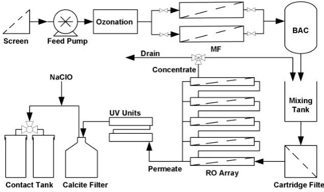
Figure 1. Schematic of the pilot plant.
2.2.2. Plant Tests and Monitoring
The AWTP was designed to achieve a water recovery of 70% at a constant feed rate of 20 L/min (1200 L/h) and could be remotely operated. The AWTP was designed to operate intermittently for a maximum of 21 h/day and had the capacity to reduce to 4 h operation every two days. It was designed to start and stop automatically and to enter standby mode when the feed tank to the treatment plant fell below a low level set point and to re‐start once the tank exceeded a high level set point. The feed water quality was monitored to ensure it met the assumed feed water quality of the design, and target and alarm levels set for feedwater quality are shown in Table 1.
The plant was commissioned for 2 months to establish remote operation, verify the detection of critical control point values, and confirm automatic start/stop operation. It also established criteria for the calibration of sensors, and the frequency required to re‐fill chemical tanks. Assessment was also made of the level and types of interventions (level of technical expertise) required to re‐start operations after critical faults. The plant typically operated for five days per week, while intermittent operation was controlled by levels in a ‘virtual’ tank so actual production and standby times were similar to what might be expected at Davis Station (i.e., 6–7 h operation and 4 h standby). A formal hand‐over process was not conducted at the end of the commissioning period, and an ongoing process of fault improvement continued.
Two samples were taken for each barrier weekly for analysing dissolved organic carbon (DOC) (measured by a Shimadzu (Chiyoda‐ku, Tokyo, Japan), TOC_V with TNM‐1 unit), total nitrogen (TN measured by Shimadzu (Chiyoda‐ku, Tokyo, Japan), TOC_V with TNM‐1 unit), total phosphate (TP, Shimadzu (Chiyoda‐ku, Tokyo, Japan), ICP2000), calcium (Shimadzu (Chiyoda‐ku, Tokyo, Japan), ICP2000) and other metals (Shimadzu (Chiyoda‐ku, Tokyo, Japan), ICP2000) for comparison with the Australian Drinking Water Guideline (ADWG). E. coli and total coliforms were tested weekly by plate counting for samples of plant feed, ozone effluent, ceramic MF filtrate, BAC filtrate, RO permeate and product water. Somatic coliphage as a surrogate for virus in the plant feed, ozonation effluent, ceramic MF filtrate, BAC filtrate and product water were analysed five times during the operation period. Biodegradable dissolved organic carbon (BDOC) of feed, ozonation effluent, ceramic MF filtrate and BAC filtrate were analysed three times during the trial by the Joret method, and were performed by Research Laboratory Services Pty Ltd. (Eltham, Victoria, Australia). The chemical consumption and plant operation time were calculated based on the data recorded by the supervisory control and data acquisition (SCADA) system. The required critical values for each barrier are listed in Table 1.
Figure 1.Schematic of the pilot plant.
2.2.2. Plant Tests and Monitoring
The AWTP was designed to achieve a water recovery of 70% at a constant feed rate of 20 L/min (1200 L/h) and could be remotely operated. The AWTP was designed to operate intermittently for a maximum of 21 h/day and had the capacity to reduce to 4 h operation every two days. It was designed to start and stop automatically and to enter standby mode when the feed tank to the treatment plant fell below a low level set point and to re-start once the tank exceeded a high level set point. The feed water quality was monitored to ensure it met the assumed feed water quality of the design, and target and alarm levels set for feedwater quality are shown in Table1.
The plant was commissioned for 2 months to establish remote operation, verify the detection of critical control point values, and confirm automatic start/stop operation. It also established criteria for the calibration of sensors, and the frequency required to re-fill chemical tanks. Assessment was also made of the level and types of interventions (level of technical expertise) required to re-start operations after critical faults. The plant typically operated for five days per week, while intermittent operation was controlled by levels in a ‘virtual’ tank so actual production and standby times were similar to what might be expected at Davis Station (i.e., 6–7 h operation and 4 h standby). A formal hand-over process was not conducted at the end of the commissioning period, and an ongoing process of fault improvement continued.
Biodegradable dissolved organic carbon (BDOC) of feed, ozonation effluent, ceramic MF filtrate and BAC filtrate were analysed three times during the trial by the Joret method, and were performed by Research Laboratory Services Pty Ltd. (Eltham, Victoria, Australia). The chemical consumption and plant operation time were calculated based on the data recorded by the supervisory control and data acquisition (SCADA) system. The required critical values for each barrier are listed in Table1.
Following operation for 6 months, SCADA faults were corrected and adjustments made to the plant based on operational performance during the first operational period. Trend analysis of operational performance was formally captured on the SCADA for each barrier in the AWTP and fault analysis was recorded in the operator log. The plant did not operate during days 160–170 (Easter holiday period) or around day 180 when serious maintenance issues at SPWWTP resulted in feed water quality exceeding the set limits. Periods of high flow because of rainfall also resulted in high feed turbidity and the plant was shut down.
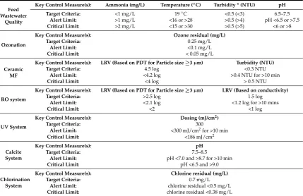
Table 1.Required critical control values for each barrier.
Feed Wastewater
Quality
Key Control Measure(s): Ammonia (mg/L) Temperature (◦C) Turbidity * (NTU) pH
Target Criteria: <1 mg/L 19◦C <0.5 (<3) 6.5–7.5 Alert Limit: >1 mg/L <16 or >28 >0.5 (>4) pH <6.5 or >7.5 Critical Limit: >2 mg/L <15 or >30 >0.5 (>5) <6 or >8
Ozonation
Key Control Measure(s): Ozone residual (mg/L)
Target Criteria: 0.25 mg/L
Alert Limit: <0.1 mg/L
Critical Limit: < 0.05 mg/L
Ceramic MF
Key Control Measure(s): LRV (Based on PDT for Particle size≥3µm) Turbidity (NTU)
Target Criteria: 4.5 log <0.3 NTU
Alert Limit: <4.2 log >0.4 NTU for >10 min
Critical Limit: <4 log > 0.5 NTU
RO system
Key Control Measure(s): LRV (Based on PDT for Particle size≥3µm) LRV (Based on conductivity)
Target Criteria: >2.5 log 1.5 log
Alert Limit: <2.1 log <1.2 log for >10 mins
Critical Limit: <2 <1 log
UV System
Key Control Measure(s): Dosing (mJ/cm2)
Target Criteria: 300
Alert Limit: <300 mJ/cm2for >10 min
Critical Limit: <186 mJ/cm2
Calcite System
Key Control Measure(s): pH
Target Criteria: 7.5–8.5
Alert Limit: pH <7.0 and >8.7 for >10 min
Critical Limit: pH <6.5 and >9.0
Chlorination System
Key Control Measure(s): Chlorine residual (mg/L)
Target Criteria: 0.7 mg/L
Alert Limit: chlorine residual <0.5 mg/L Critical Limit: chlorine residual <0.38 mg/L
Notes: * Turbidity values are for the Davis Station MBR effluent; Values in brackets are for Selfs Point wastewater effluent.
2.2.3. Plant Challenge for Disinfection By-Products
Water2017,9, 94 7 of 25
Water) and analysed for a variety of DPBs (bromate (BrO3−), iodate (IO3−), Adsorbable Organic Halides (AOCl, AOBr and AOI), trihalomethanes (THMs) and haloacetic acids (HAAs)). Duplicate measurements were carried out for all samples.
Samples (24) were collected in amber bottles. Residual ozone in the Post ozone and Post MF samples was quenched with sodium sulphite during collection, while Product Water samples were quenched for chlorine.
Ion chromatography (IC) (Dionex (Sunnyvale, CA, USA) ICS3000 ion chromatograph) was used to analyse for halides (Br− and I−) and oxyhalides (BrO3− and IO3−). The IC was fitted with an anion exchange column (Dionex IonPac®(Sunnyvale, CA, USA) AS9-HC 4×250 mm), used sodium carbonate as the eluent and utilised conductivity and UV for detection. Filtered samples (500µL) were injected into the IC and the anions were measured simultaneously. Br−and I−were detected using conductivity. BrO3−and IO3−were detected using an online post-column reaction (using acidified potassium iodide, catalysed by heptamolybdate) with UV/Vis detection.
The method of Kristiana, et al. [7] was used to analyse for specific adsorbable organic halides (AOCl, AOBr and AOI). Acidified (pH 2) 50 mL of samples were passed through two activated carbon columns in series, the activated carbon columns combusted (Mitsubishi AQF-100), the hydrogen halide gases collected in MilliQ water and subsequently analysed in an IC system using an anion exchange column (Dionex IonPac®(Sunnyvale, CA, USA) AS19-HC 4×250 mm) and conductivity detector.
Head-space solid phase micro-extraction (SPME), followed by gas chromatography separation and mass spectrometry detection (GC–MS) was used to analyse for 10 trihalomethanes (THMs) according to a published method [8]. The THMs analysed were Iodoform (CHI3), Bromodiiodomethane (CHBrI2), Dichloroiodomethane (CHCl2I), Bromochloroiodomethane (CHBrClI), Dibromoiodomethane (CHBr2I), Chlorodiiodomethane (CHClI2), Bromoform (CHBr3), Bromodichloromethane (CHBrCl2), Chlorodibromomethane (CHBr2Cl), and Chloroform (CHCl3).
Liquid–liquid extraction (LLE) with methyl-tert-butyl-ether (MtBE), subsequent derivatisation with acidic methanol, followed by quantification using GC-was used to analyse the haloacetic acid concentrations. The nine haloacetic acids (HAAs) measured were Bromodichloroacetic acid (BDCAA), Tribromoacetic acid (TBAA), Dibromoacetic acid (DBAA), Chlorodibromoacetic acid (CDBAA), Bromochloroacetic acid (BCAA), Bromoacetic acid (MBAA), Trichloroacetic acid (TCAA), Dichloroacetic acid (DCAA) and Chloroacetic acid (MCAA).
Specific ultraviolet absorbance at 254 nm (SUVA254), defined as the ultra-violet absorbance at 254 nm (UV254) divided by dissolved organic carbon (DOC) concentration, was measured for all DBP Plant Feed and Post Ozone samples. SUVA254 was used as a measure of the aromatic content of the organic matter (i.e., strong reactive sites). A Shimadzu TOC-Vws Total Organic Carbon (TOC) analyser was used to measure DOC concentrations and UV254was measured using a Cary 60 UV-Vis Spectrophotometer (Agilent Technologies, Santa Clara, CA, USA).
2.2.4. Screening for Trace Organic Chemicals (TrOCs)
An Automated Identification and Quantification System database method (AIQS-DB) was linked to gas chromatographic–mass spectrometric (GC–MS) and liquid chromatographic-time of flight mass spectrometric (LC-TOF-MS) methods to allow the determination of more than 1250 trace organic chemicals (TrOCs) in extracted water samples. These methods differ from many current operations, where a few chemicals (surrogates) are often chosen to be representative of many, because of the difficulty and cost of assessment of the very large range of chemicals that could be present in secondary effluent.
The AIQS-DB method uses internal standard calibration curves, obtained under set operating conditions, to identify and quantify chemical substances using retention times and mass spectra. The GC–MS or LC-TOF-MS instrument conditions are required to be adjusted to the designated conditions used to compile the database in order to obtain accurate results. The results obtained from performance check standards were evaluated against three criteria (spectrum validity, inertness of column and inlet liner, and stability of response) and the difference between the predicted and actual retention times will be less than 3 s. The method detection limits (MDL) for target substances are estimated from the concentration ratio and the instrument detection limit (IDL) of model compounds and are in the range 0.01 to 0.1µg/L for GC–MS, and 2.5–5 ng/L for LC-TOF-MS. The AIQS-DB GC–MS method can detect 940 semi-volatile substances including a variety of polychlorinated biphenyl compounds (PCBs); halogenated and non-halogenated hydrocarbons; pharmaceutical and personal care products (PPCPs); polycyclic aromatic hydrocarbons (PAHs); and agricultural compounds. The AIQS-DB LC-TOF-MS method can analyse 265 polar and non-volatile compounds, including 180 agricultural compounds and 70 pharmaceuticals.
3. Results
3.1. Feed Water Quality
Ammonia and TN data for the feedwater during the AWTP trials are given in Figure2. The data shows that the ammonia concentration was below the target feedwater criteria for 14 days and increased above the critical limit of 5 mg/L after the SPWWTP doubled the required inflow rate of the settlers (maintenance on one settler). The feedwater ammonia levels returned to <1 mg/L after 50 days. However, another two ammonia feed concentration peaks were also found around 150 days and 210 days. The DOC (7.3–9.4 mg/L), temperature (>15◦C) and pH (6.5–7.5) did not vary significantly. Turbidity, as shown in Figure2, was usually between 1 and 3 NTU in the feedwater, but during wet weather events this increased to 3–5 NTU. The ammonia, DOC and TN data were obtained from grab samples of the feedwater, while the turbidity, temperature and pH were collected from on-line instruments. During the high ammonia and TN period, the turbidity values averaged 2.5 NTU. Peaks in turbidity were recorded at 5 NTU and on occasion at 10–15 NTU. These turbidity results suggest that larger particles were present in the feed. The turbidity values were measured in the effluent channel. The feed was then screened (2 mm) before it entered the plant. Hence, some of the turbidity may have been removed before entering the AWTP.
Water 2017, 9, 94 8 of 25
(IDL) of model compounds and are in the range 0.01 to 0.1 μg/L for GC–MS, and 2.5–5 ng/L for LC‐TOF‐MS. The AIQS‐DB GC–MS method can detect 940 semi‐volatile substances including a variety of polychlorinated biphenyl compounds (PCBs); halogenated and non‐halogenated hydrocarbons; pharmaceutical and personal care products (PPCPs); polycyclic aromatic hydrocarbons (PAHs); and agricultural compounds. The AIQS‐DB LC‐TOF‐MS method can analyse 265 polar and non‐volatile compounds, including 180 agricultural compounds and 70 pharmaceuticals.
3. Results
3.1. Feed Water Quality
Ammonia and TN data for the feedwater during the AWTP trials are given in Figure 2. The data shows that the ammonia concentration was below the target feedwater criteria for 14 days and increased above the critical limit of 5 mg/L after the SPWWTP doubled the required inflow rate of the settlers (maintenance on one settler). The feedwater ammonia levels returned to <1 mg/L after 50 days. However, another two ammonia feed concentration peaks were also found around 150 days and 210 days. The DOC (7.3–9.4 mg/L), temperature (>15 °C) and pH (6.5–7.5) did not vary significantly. Turbidity, as shown in Figure 2, was usually between 1 and 3 NTU in the feedwater, but during wet weather events this increased to 3–5 NTU. The ammonia, DOC and TN data were obtained from grab samples of the feedwater, while the turbidity, temperature and pH were collected from on‐line instruments. During the high ammonia and TN period, the turbidity values averaged 2.5 NTU. Peaks in turbidity were recorded at 5 NTU and on occasion at 10–15 NTU. These turbidity results suggest that larger particles were present in the feed. The turbidity values were measured in the effluent channel. The feed was then screened (2 mm) before it entered the plant. Hence, some of the turbidity may have been removed before entering the AWTP.
Figure 2. Feedwater ammonia, DOC and TN concentration.
In total, for about 90 days of the 230 test days, the ammonia concentrations and Turbidity were not in the CCP required range, and all the other CCPs met the required values for the feedwater.
The measured metal concentration of the feed water is shown in Table 2. It is shown that all metals of interest for ADWG in the feed water were lower than the guideline value.
0 2 4 6 8 10 12 14 16 18
0 5 10 15 20 25 30
0 50 100 150 200
C
o
n
cent
ra
ti
o
n
(mg
/L)
Tu
rb
id
ity
(NT
U
)
Time (day)
Turbidity Feed Ammonia Feed TN
Water2017,9, 94 9 of 25
In total, for about 90 days of the 230 test days, the ammonia concentrations and Turbidity were not in the CCP required range, and all the other CCPs met the required values for the feedwater.
The measured metal concentration of the feed water is shown in Table2. It is shown that all metals of interest for ADWG in the feed water were lower than the guideline value.
Table 2.Metal concentration in the feed water.
Metal ADWG Value (mg/L) Concentration (mg/L)
Aluminium 0.1 <0.03
Antimony 0.003 Not detectable
Arsenic 0.01 <0.009
Barium 2 <0.008
Beryllium 0.006 Not detectable
Boron 4 <0.06
Cadmium 0.002 Under detection limit
Chromium 0.05 <0.03
Copper 2 <0.006
Iron 0.3 <0.25
Lead 0.01 Under detection limit
Manganese 0.1 <0.05
Mercury 0.001 Not detectable
Nickel 0.02 <0.005
Selenium 0.01 <0.009
Silver 0.1 <0.009
3.2. Ozonation Barrier
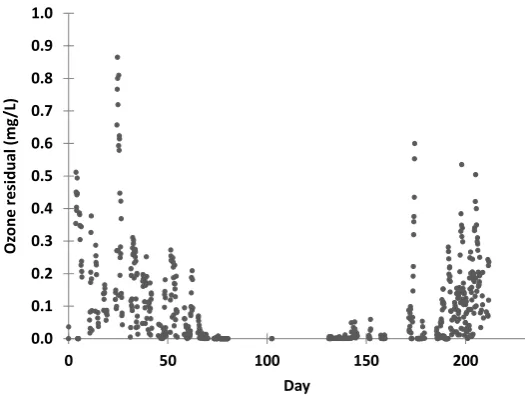
The ozone residual at the outlet of the ozone contact tank is shown in Figure3, with about 50% of the measured ozone residual value less than the critical value (0.01 mg/L) and 37% greater than the targeted value (0.1 mg/L). It was found that the depletion of the ozone was directly related to the turbidity rather than the ammonia concentration [11].
Water 2017, 9, 94 9 of 25
Table 2. Metal concentration in the feed water.
Metal ADWG Value (mg/L) Concentration (mg/L)
Aluminium 0.1 <0.03
Antimony 0.003 Not detectable
Arsenic 0.01 <0.009
Barium 2 <0.008
Beryllium 0.006 Not detectable
Boron 4 <0.06
Cadmium 0.002 Under detection limit
Chromium 0.05 <0.03
Copper 2 <0.006
Iron 0.3 <0.25
Lead 0.01 Under detection limit
Manganese 0.1 <0.05
Mercury 0.001 Not detectable
Nickel 0.02 <0.005
Selenium 0.01 <0.009
Silver 0.1 <0.009
3.2. Ozonation Barrier
The ozone residual at the outlet of the ozone contact tank is shown in Figure 3, with about 50% of the measured ozone residual value less than the critical value (0.01 mg/L) and 37% greater than the targeted value (0.1 mg/L). It was found that the depletion of the ozone was directly related to the turbidity rather than the ammonia concentration [11].
Figure 3. Ozone residual at the ozone contact tank outlet.
The Davis Station MBR should produce a reliable, low turbidity feedwater that will enable an ozone residual to be maintained, and subsequently allow the use of CT values set by the US EPA Long‐Term 2 Enhanced surface water treatment rule to define the LRV value.
Figure 4 shows the variation of ozone residual along with the varying pressure of the ozone contact tank. The pressure in the ozone contactor varied as a result of downstream fouling of the ceramic MF membrane resulting in a higher upstream pressure and increasing the dissolved ozone concentration in the water. This suggests that controlling the pressure of the ozone system by either placing a control valve on ceramic MF outlet or by including a pressure control valve on the ozone outlet and using a separate ceramic MF feed pump would provide greater control of ozone
0.0 0.1 0.2 0.3 0.4 0.5 0.6 0.7 0.8 0.9 1.0
0 50 100 150 200
Oz
one
re
si
dua
l
(mg
/L)
Day
Figure 3.Ozone residual at the ozone contact tank outlet.
The Davis Station MBR should produce a reliable, low turbidity feedwater that will enable an ozone residual to be maintained, and subsequently allow the use of CT values set by the US EPA Long-Term 2 Enhanced surface water treatment rule to define the LRV value.
concentration in the water. This suggests that controlling the pressure of the ozone system by either placing a control valve on ceramic MF outlet or by including a pressure control valve on the ozone outlet and using a separate ceramic MF feed pump would provide greater control of ozone residuals for high turbidity waters. However, the short trial timespan prevented the installation of such control and inclusion of a MBR upstream of the ozone unit at Davis Station will eliminate high turbidity feed to the ozone system and hence the need for such control.
Water 2017, 9, 94 10 of 25
residuals for high turbidity waters. However, the short trial timespan prevented the installation of such control and inclusion of a MBR upstream of the ozone unit at Davis Station will eliminate high turbidity feed to the ozone system and hence the need for such control.
Figure 4. Relationship between the contact tank pressure and ozone residual.
The ratio of produced and transferred ozone to the wastewater is listed in Table 3. The ozone transferred to the feed water was in the range of 60% to 80%, and did not show a clear relationship to the pressure in the contact tank. However, maintaining the dosed ozone >11.7 mg/L was sufficient to ensure >2 LRV for bacteria and virus [11].
Table 3. Ozone transferred into the contact tank.
Day Pressure in Contact Tank (bar)
Temperature (°C)
Transferred Ozone (mg/L)
Produced Ozone (mg/L)
Percentage (%)
65 0.3 20.5 13.5 20.7 65.0
126 0.4 21.4 14.8 20.6 71.9
140 0.4 22.7 11.7 19.3 60.5
155 0.7 22.7 14.9 20.3 73.3
212 0.4 19.7 16.9 20.8 81.4
224 0.4 18.0 12.9 20.9 61.8
3.3. Ceramic MF
The PDT rates of the two ceramic membranes were all below the 1.4 kPa/min limit for the entire test period, apart from when there were leaking valves [11]. The PDT data always met the required CCP limit, confirming the reliability of the ceramic MF membranes for attaining this CCP. The filtrate turbidity from the ceramic MF measured by the online turbidity meter and the handheld meter are shown in Figure 5. The turbidity readings of the handheld meter all met the target value. However, the reading of the online turbidity meter was occasionally unable to meet the target value, and would trigger an alarm if used as a critical control point. The sample point was moved to the BAC weir from the 123th day to avoid possible influence from air bubbles in the filtrate. The initial on‐line turbidity readings remained high, but after 10 min filtration, the turbidity readings were less than 0.2 NTU and mostly less than 0.1 NTU demonstrating the high quality filtration performance of the ceramic MF membranes.
0.4 0.9 1.4 1.9 2.4 2.9
0 0.1 0.2 0.3 0.4 0.5 0.6 0.7 0.8
525 530 535 540 545
Pressure
(Bar)
Oz
o
n
e
re
si
dual
(m
g/
L)
Time (h)
Ozone residual
Contact tank pressure
Figure 4.Relationship between the contact tank pressure and ozone residual.
The ratio of produced and transferred ozone to the wastewater is listed in Table3. The ozone transferred to the feed water was in the range of 60% to 80%, and did not show a clear relationship to the pressure in the contact tank. However, maintaining the dosed ozone >11.7 mg/L was sufficient to ensure >2 LRV for bacteria and virus [11].
Table 3.Ozone transferred into the contact tank.
Day Pressure in Contact Tank (bar)
Temperature (◦C)
Transferred Ozone (mg/L)
Produced Ozone (mg/L)
Percentage (%)
65 0.3 20.5 13.5 20.7 65.0
126 0.4 21.4 14.8 20.6 71.9
140 0.4 22.7 11.7 19.3 60.5
155 0.7 22.7 14.9 20.3 73.3
212 0.4 19.7 16.9 20.8 81.4
224 0.4 18.0 12.9 20.9 61.8
3.3. Ceramic MF
The PDT rates of the two ceramic membranes were all below the 1.4 kPa/min limit for the entire test period, apart from when there were leaking valves [11]. The PDT data always met the required CCP limit, confirming the reliability of the ceramic MF membranes for attaining this CCP.
Water2017,9, 94 11 of 25
Water 2017, 9, 94 11 of 25
Figure 5. Turbidity of the ceramic MF filtrate (● handheld turbidity readings, + on‐line turbidity readings).
No long‐term fouling of the ceramic MF was observed over the entire operational period, as shown by the pressure recovery data in Figure 6. The feed pressure to the ceramic MF units increased as they fouled during filtration, but the feed pressure returned to the initial value upon backwashing and with occasional chemically enhanced backwashing. This confirms that the approach of applying a 100 mg/L NaOCl CEB was sufficient to prevent the requirement for a CIP.
Figure 6. Feed pressure to MF number 1 over the life of the demonstration trials. The continuous line shows the initial feed pressure at the start of the trials.
3.4. Biological Activated Carbon (BAC)
An indication of bacterial concentrations on the activated carbon from three depths within the BAC were used to confirm that there was biological activity within the BAC. Activated carbon samples were taken from the top, middle and bottom of the BAC and the indicative bacterial concentrations measured by Research Laboratory Services Pty Ltd. Bacterial concentrations were determined by washing the bacteria from the surface of the activated carbon using a standard washing procedure, and growing the bacteria on agar plates. The measured microbial concentrations were 312,500 cfu/100 mL at the top; 153,333 cfu/100 mL in the middle and 103,667 cfu/100 mL at the bottom of the BAC. These bacterial concentrations were high and reduced from
0.0001 0.0010 0.0100 0.1000 1.0000 10.0000
0 50 100 150 200 250
Tu rb id ity (N TU) Day
0.3 NTU 123thday
0.0 0.5 1.0 1.5 2.0 2.5 3.0 3.5
0 20 40 60 80 100 120 140 160
Fe ed Pressu re (b ar) Day 0.197 bar 48 83 139 1 21 30 69 119
Figure 5.Turbidity of the ceramic MF filtrate ( handheld turbidity readings, + on-line turbidity readings).
No long-term fouling of the ceramic MF was observed over the entire operational period, as shown by the pressure recovery data in Figure6. The feed pressure to the ceramic MF units increased as they fouled during filtration, but the feed pressure returned to the initial value upon backwashing and with occasional chemically enhanced backwashing. This confirms that the approach of applying a 100 mg/L NaOCl CEB was sufficient to prevent the requirement for a CIP.
Water 2017, 9, 94 11 of 25
Figure 5. Turbidity of the ceramic MF filtrate (● handheld turbidity readings, + on‐line turbidity readings).
No long‐term fouling of the ceramic MF was observed over the entire operational period, as shown by the pressure recovery data in Figure 6. The feed pressure to the ceramic MF units increased as they fouled during filtration, but the feed pressure returned to the initial value upon backwashing and with occasional chemically enhanced backwashing. This confirms that the approach of applying a 100 mg/L NaOCl CEB was sufficient to prevent the requirement for a CIP.
Figure 6. Feed pressure to MF number 1 over the life of the demonstration trials. The continuous line shows the initial feed pressure at the start of the trials.
3.4. Biological Activated Carbon (BAC)
An indication of bacterial concentrations on the activated carbon from three depths within the BAC were used to confirm that there was biological activity within the BAC. Activated carbon samples were taken from the top, middle and bottom of the BAC and the indicative bacterial concentrations measured by Research Laboratory Services Pty Ltd. Bacterial concentrations were determined by washing the bacteria from the surface of the activated carbon using a standard washing procedure, and growing the bacteria on agar plates. The measured microbial concentrations were 312,500 cfu/100 mL at the top; 153,333 cfu/100 mL in the middle and 103,667 cfu/100 mL at the bottom of the BAC. These bacterial concentrations were high and reduced from
0.0001 0.0010 0.0100 0.1000 1.0000 10.0000
0 50 100 150 200 250
Tu rb id ity (N TU) Day
0.3 NTU 123thday
0.0 0.5 1.0 1.5 2.0 2.5 3.0 3.5
0 20 40 60 80 100 120 140 160
Fe ed Pressu re (b ar) Day 0.197 bar 48 83 139 1 21 30 69 119
Figure 6.Feed pressure to MF number 1 over the life of the demonstration trials. The continuous line
shows the initial feed pressure at the start of the trials.
3.4. Biological Activated Carbon (BAC)
These bacterial concentrations were high and reduced from the top to the bottom, consistent with declining food (biodegradable organic matter) availability as water flows through the BAC.
The head loss of the BAC filter is shown in Figure7. Based on the data, it is seen that during the trial, the BAC filter triggered the backwash alarm twice. However, after day 123 of the test, a new protocol was used whereby a backwash was triggered on treated water volume (300 m3). The BAC filter did not show significant head loss from this point forward.
the top to the bottom, consistent with declining food (biodegradable organic matter) availability as water flows through the BAC.
The head loss of the BAC filter is shown in Figure 7. Based on the data, it is seen that during the trial, the BAC filter triggered the backwash alarm twice. However, after day 123 of the test, a new protocol was used whereby a backwash was triggered on treated water volume (300 m3). The BAC filter did not show significant head loss from this point forward.
Figure 7. Head loss of the BAC filter (1 and 2 indicate times when the backwash was triggered because of high pressure drop across the BAC).
Both adsorption of organic matter and biological activity can remove organic carbon from solution as it travels through the BAC. In Figure 8, the DOC reduction over time is shown. DOC was consistently reduced by 30%–50% in the effluent in comparison with the influent.
Figure 8. DOC removal across the BAC with time.
Performance monitoring of the BAC utilised on‐line turbidity measurements of the BAC effluent. Turbidity values should be low and increases in turbidity may be indicative of changes in biological activity. A high turbidity (>0.2 NTU) would trigger a plant shutdown. A typical turbidity trend recorded by the online turbidity meter is shown in Figure 9. High turbidity was recorded when the plant transited from standby mode to operation mode but stabilised over the first 20 min after commencing operation. This time is similar to the EBCT. However, a small spike, over
0 5 10 15 20 25 30
0 50 100 150 200 250
Pr
essu
re
(mb
ar)
Day
1 2
0 10 20 30 40 50 60
0 30 60 90 120 150 180 210 240 270
DOC
Re
d
u
ct
io
n
(%)
Day
Figure 7.Head loss of the BAC filter (1 and 2 indicate times when the backwash was triggered because
of high pressure drop across the BAC).
Both adsorption of organic matter and biological activity can remove organic carbon from solution as it travels through the BAC. In Figure8, the DOC reduction over time is shown. DOC was consistently reduced by 30%–50% in the effluent in comparison with the influent.
Water 2017, 9, 94 12 of 25
the top to the bottom, consistent with declining food (biodegradable organic matter) availability as water flows through the BAC.
The head loss of the BAC filter is shown in Figure 7. Based on the data, it is seen that during the trial, the BAC filter triggered the backwash alarm twice. However, after day 123 of the test, a new protocol was used whereby a backwash was triggered on treated water volume (300 m3). The BAC filter did not show significant head loss from this point forward.
Figure 7. Head loss of the BAC filter (1 and 2 indicate times when the backwash was triggered because of high pressure drop across the BAC).
Both adsorption of organic matter and biological activity can remove organic carbon from solution as it travels through the BAC. In Figure 8, the DOC reduction over time is shown. DOC was consistently reduced by 30%–50% in the effluent in comparison with the influent.
Figure 8. DOC removal across the BAC with time.
Performance monitoring of the BAC utilised on‐line turbidity measurements of the BAC effluent. Turbidity values should be low and increases in turbidity may be indicative of changes in biological activity. A high turbidity (>0.2 NTU) would trigger a plant shutdown. A typical turbidity trend recorded by the online turbidity meter is shown in Figure 9. High turbidity was recorded when the plant transited from standby mode to operation mode but stabilised over the first 20 min after commencing operation. This time is similar to the EBCT. However, a small spike, over
0 5 10 15 20 25 30
0 50 100 150 200 250
Pr
essu
re
(mb
ar)
Day
1 2
0 10 20 30 40 50 60
0 30 60 90 120 150 180 210 240 270
DOC
Re
d
u
ct
io
n
(%)
Day
Figure 8.DOC removal across the BAC with time.
Water2017,9, 94 13 of 25
commencing operation. This time is similar to the EBCT. However, a small spike, over 0.2 NTU, was also observed corresponding to backwash of the ceramic MF. It was caused by vibrational disturbance due to the sudden pressure released in the ceramic MF backwash process. Therefore, these turbidity spikes were ignored in the SCADA system to avoid regular plant shutdown.
Water 2017, 9, 94 13 of 25
0.2 NTU, was also observed corresponding to backwash of the ceramic MF. It was caused by vibrational disturbance due to the sudden pressure released in the ceramic MF backwash process. Therefore, these turbidity spikes were ignored in the SCADA system to avoid regular plant shutdown.
Figure 9. Typical turbidity values in the BAC filtrate.
Decreases in pH and alkalinity across the BAC can indicate that nitrification is occurring within the filter. Alkalinity and pH changes across the BAC were measured for two months and the results are shown in Table 4. The results indicate reductions in alkalinity and pH, confirming that nitrification was taking place. This is probably related to the intermittent operation of the BAC and insufficient aeration during standby operation.
Table 4. pH and alkalinity changes across the BAC.
Day pH Δ pH Alkalinity (mg/L CaCO3) Δ Alkalinity (mg/L CaCO3) Influent Effluent
120 7.65 7.56 0.09 / / /
127 / / / 165 157 8
134 7.74 7.62 0.12 172 163 9
141 / / / 163 155 8
148 7.57 7.18 0.39 166 140 26 163 7.57 7.41 0.16 138 128 10 168 7.04 6.87 0.17 152 126 26 183 7.06 7.04 0.02 135 128 7
Notes: / no data available.
3.5. RO Barrier
The RO system consisted of five‐element array preceded by a 0.1 μm cartridge filter. The CCPs of RO were conductivity and PDTs, which were all in the required value range during the testing period. The RO was also challenged with Rhodamine WT, and the results are shown in Figure 10. The RO membrane barrier was able to achieve greater than 2.1 LRV for Rhodamine WT, which indicates that the membrane was able to achieve 2 LRV for virus, although only 1 LRV was claimed based on on‐line conductivity measurements.
0.0 0.1 0.2 0.3 0.4 0.5 0.6 0.7 0.8 0.9 1.0
0 200 400 600 800 1000
Tu
rb
id
it
y
(N
T
U
)
Time (min)
Influence from
MF backwash
Initial 20 min
Figure 9.Typical turbidity values in the BAC filtrate.
Decreases in pH and alkalinity across the BAC can indicate that nitrification is occurring within the filter. Alkalinity and pH changes across the BAC were measured for two months and the results are shown in Table4. The results indicate reductions in alkalinity and pH, confirming that nitrification was taking place. This is probably related to the intermittent operation of the BAC and insufficient aeration during standby operation.
Table 4.pH and alkalinity changes across the BAC.
Day pH ∆pH Alkalinity (mg/L CaCO3) ∆Alkalinity (mg/L CaCO3)
Influent Effluent
120 7.65 7.56 0.09 / / /
127 / / / 165 157 8
134 7.74 7.62 0.12 172 163 9
141 / / / 163 155 8
148 7.57 7.18 0.39 166 140 26
163 7.57 7.41 0.16 138 128 10
168 7.04 6.87 0.17 152 126 26
183 7.06 7.04 0.02 135 128 7
Notes: / no data available.
3.5. RO Barrier
Figure10. Rhodamine WT concentration in RO permeate and the measured Rhodamine WT LRV across the RO process.
The pressure of the cartridge filter immediately upstream of the RO was also monitored, since the blockage of the filter would lower the suction head, causing the RO high pressure pump to shut down if the pressure was less than −80 kPa. Figure 11 shows three recorded pressure drops of the cartridge filter. Based on the fitting equations in Figure 11, the cartridge filter was able to be used for 7.5 days.
Figure 11. Pressure drop across the cartridge filter.
A fouled cartridge filter underwent an autopsy and was shown to be extensively fouled by black particles with little Mn present. It was concluded that the main foulant was carbon particles, as these particles were also observed at the bottom of the mixing tank. These fine carbon particles were assumed to be broken activated carbon. The frequent replacement of cartridge filters may be problematic for some locations, but was deemed acceptable by the AAD as the process of cartridge filter replacement could be easily achieved by their operator. However, for other locations, such frequent replacement may not be acceptable, and placement of the BAC prior to the ceramic MF may be appropriate.
Fouling of the RO membrane also occurred and a CIP was required after a period of 4–5 months, indicating a need for 2–3 CIPs each year [11]. A fouled RO membrane was also subjected to autopsy. The average foulant load was 4 g/m2 and the ratio of inorganic matter to the organic matter was 9:100. This is consistent with the foulant layer being predominantly biofouling.
10 15 20 25 30 35 40 2 2.1 2.2 2.3 2.4 2.5
3000 3500 4000 4500 5000 5500 6000
Per m eate concentrati o n (µ g/ L) LRV
Feed concentration (µg/L)
LRV
Permeate concentration
y = ‐1.21E‐08x2+ 4.32E‐05x ‐1.88E‐01 y = ‐8.14E‐09x2‐3.98E‐06x ‐8.48E‐02 y = ‐8.65E‐09x2+ 6.84E‐06x ‐7.98E‐02
‐0.6 ‐0.5 ‐0.4 ‐0.3 ‐0.2 ‐0.1 0
0 1000 2000 3000 4000 5000 6000 7000 8000
Pr e ssu re (b ar)
Time (min)
A
B
C
Figure 10. Rhodamine WT concentration in RO permeate and the measured Rhodamine WT LRV
across the RO process.
The pressure of the cartridge filter immediately upstream of the RO was also monitored, since the blockage of the filter would lower the suction head, causing the RO high pressure pump to shut down if the pressure was less than−80 kPa. Figure11shows three recorded pressure drops of the cartridge filter. Based on the fitting equations in Figure11, the cartridge filter was able to be used for 7.5 days.
Figure10. Rhodamine WT concentration in RO permeate and the measured Rhodamine WT LRV across the RO process.
The pressure of the cartridge filter immediately upstream of the RO was also monitored, since the blockage of the filter would lower the suction head, causing the RO high pressure pump to shut down if the pressure was less than −80 kPa. Figure 11 shows three recorded pressure drops of the cartridge filter. Based on the fitting equations in Figure 11, the cartridge filter was able to be used for 7.5 days.
Figure 11. Pressure drop across the cartridge filter.
A fouled cartridge filter underwent an autopsy and was shown to be extensively fouled by black particles with little Mn present. It was concluded that the main foulant was carbon particles, as these particles were also observed at the bottom of the mixing tank. These fine carbon particles were assumed to be broken activated carbon. The frequent replacement of cartridge filters may be problematic for some locations, but was deemed acceptable by the AAD as the process of cartridge filter replacement could be easily achieved by their operator. However, for other locations, such frequent replacement may not be acceptable, and placement of the BAC prior to the ceramic MF may be appropriate.
Fouling of the RO membrane also occurred and a CIP was required after a period of 4–5 months, indicating a need for 2–3 CIPs each year [11]. A fouled RO membrane was also subjected to autopsy. The average foulant load was 4 g/m2 and the ratio of inorganic matter to the organic matter was 9:100. This is consistent with the foulant layer being predominantly biofouling.
10 15 20 25 30 35 40 2 2.1 2.2 2.3 2.4 2.5
3000 3500 4000 4500 5000 5500 6000
Per m eate concentrati o n (µ g/ L) LRV
Feed concentration (µg/L)
LRV
Permeate concentration
y = ‐1.21E‐08x2+ 4.32E‐05x ‐1.88E‐01 y = ‐8.14E‐09x2‐3.98E‐06x ‐8.48E‐02
y = ‐8.65E‐09x2+ 6.84E‐06x ‐7.98E‐02
‐0.6 ‐0.5 ‐0.4 ‐0.3 ‐0.2 ‐0.1 0
0 1000 2000 3000 4000 5000 6000 7000 8000
Pr e ssu re (b ar)
Time (min)
A
B
C
Figure 11.Pressure drop across the cartridge filter.
A fouled cartridge filter underwent an autopsy and was shown to be extensively fouled by black particles with little Mn present. It was concluded that the main foulant was carbon particles, as these particles were also observed at the bottom of the mixing tank. These fine carbon particles were assumed to be broken activated carbon. The frequent replacement of cartridge filters may be problematic for some locations, but was deemed acceptable by the AAD as the process of cartridge filter replacement could be easily achieved by their operator. However, for other locations, such frequent replacement may not be acceptable, and placement of the BAC prior to the ceramic MF may be appropriate.
Water2017,9, 94 15 of 25
During the autopsy, it was apparent that the fouling layer could be simply removed by wiping the membrane surface. Ozone oxidation is known to oxidise membrane foulants such as protein rich, aromatic, and hydrophobic organic compounds, and the oxidation of these compounds may result in easier membrane cleaning [12].
A PDT was used to verify the integrity of the RO membranes with respect to protozoa, and the results are shown in [11]. The RO PDT confirmed >2 LRV removal across the RO membrane system for the test period. No statistically relevant decrease in RO performance was detected as a result of the PDT test.
3.6. Ultraviolet (UV) Disinfection
The T10 of the two UV units connected in series was 2.2 min, as shown in Figure12. The online measured UVC intensities of both UV units were greater than 90 w/m2. Therefore, the dosing for each unit is about 600 mJ/cm2, which is much greater than the critical value of 186 mJ/cm2.
Water 2017, 9, 94 15 of 25
During the autopsy, it was apparent that the fouling layer could be simply removed by wiping the membrane surface. Ozone oxidation is known to oxidise membrane foulants such as protein rich, aromatic, and hydrophobic organic compounds, and the oxidation of these compounds may result in easier membrane cleaning [12].
A PDT was used to verify the integrity of the RO membranes with respect to protozoa, and the results are shown in [11]. The RO PDT confirmed >2 LRV removal across the RO membrane system for the test period. No statistically relevant decrease in RO performance was detected as a result of the PDT test.
3.6. Ultraviolet (UV) Disinfection
The T10 of the two UV units connected in series was 2.2 min, as shown in Figure 12. The online measured UVC intensities of both UV units were greater than 90 w/m2. Therefore, the dosing for each unit is about 600 mJ/cm2, which is much greater than the critical value of 186 mJ/cm2.
Figure 12. The residency time of the two UV units.
The UV units were problem free for all the testing period and the decayed lamp intensity at the end of the test was greater than 94% of the starting intensity.
3.7. Calcite Contactor
The average calcium concentration in the post‐contactor water was 80 mg/L, and the contactor required additional calcite every 3–4 months. However, the calcium concentration changed with time and consequently the stability of the water also varied as it related to the calcium concentration, temperature, pH and alkalinity. The water stability was determined by calculating the calcium carbonate precipitation potential (CCPP) and the Langelier Saturation Index (LSI) from grab samples taken weekly and the on‐line pH data in the post calcite contactor line.
Figure 13 shows the measured pH, alkalinity and total dissolved solids (TDS) against time. This data, along with the temperature, was used to calculate the CCPP and LSI values. The CCPP values were all below 0, and three points were significantly lower than 20 mg/L (−88, −64, −52 mg/L). The three outliers were believed to have arisen from pH measurement errors, as pH was hard to measure occasionally. Ignoring these three outliers resulted in an average CCPP of −8.55 mg/L CaCO3 that corresponds to mildly aggressive water, with most CCPP data being between −2 to −12 mg/L CaCO3. Calculated LSI values also indicated mildly aggressive water with values between −0.5 and −1.3. The amount of water processed by the calcite contactor between re‐filling events was estimated to be 600,000 L of water.
y = 8.65E‐05x2‐1.73E‐02x + 8.71E‐01 R² = 1.00E+00
y = 5.71E‐05x2‐1.04E‐02x + 4.73E‐01 R² = 9.99E‐01
0.0 0.1 0.2 0.3 0.4
100 110 120 130 140 150 160 170
Time (s)
First
Second 2.2 min
Figure 12.The residency time of the two UV units.
The UV units were problem free for all the testing period and the decayed lamp intensity at the end of the test was greater than 94% of the starting intensity.
3.7. Calcite Contactor
The average calcium concentration in the post-contactor water was 80 mg/L, and the contactor required additional calcite every 3–4 months. However, the calcium concentration changed with time and consequently the stability of the water also varied as it related to the calcium concentration, temperature, pH and alkalinity. The water stability was determined by calculating the calcium carbonate precipitation potential (CCPP) and the Langelier Saturation Index (LSI) from grab samples taken weekly and the on-line pH data in the post calcite contactor line.
Figure13 shows the measured pH, alkalinity and total dissolved solids (TDS) against time. This data, along with the temperature, was used to calculate the CCPP and LSI values. The CCPP values were all below 0, and three points were significantly lower than 20 mg/L (−88,−64,−52 mg/L). The three outliers were believed to have arisen from pH measurement errors, as pH was hard to measure occasionally. Ignoring these three outliers resulted in an average CCPP of−8.55 mg/L CaCO3 that corresponds to mildly aggressive water, with most CCPP data being between−2 to−12 mg/L CaCO3. Calculated LSI values also indicated mildly aggressive water with values between−0.5 and