Failure Rate of Bit-flipping Decoding of LDPC
Codes with Cryptographic Applications
Paolo Santini1,2, Alessandro Barenghi3, Gerardo Pelosi3, Marco Baldi1, and Franco Chiaraluce1
1 Universit`a Politecnica delle Marche 2
Florida Atlantic University
3 Politecnico di Milano
[email protected], {alessandro.barenghi, gerardo.pelosi}@polimi.it,
{m.baldi, f.chiaraluce}@univpm.it
Abstract. Characterizing the decoding failure rate of iteratively de-coded Low- and Moderate-Density Parity Check (LDPC/MDPC) codes is paramount to build cryptosystems based on them, able to achieve in-distinguishability under adaptive chosen ciphertext attacks. In this pa-per, we provide a statistical worst-case analysis of our proposed iterative decoder obtained through a simple modification of the classic in-place bit-flipping decoder. This worst case analysis allows both to derive the worst-case behaviour of an LDPC/MDPC code picked among the family with the same length, rate and number of parity checks, and a code-specific bound on the decoding failure rate. The former result allows us to build a code-based cryptosystem enjoing theδ-correctness property required by IND-CCA2 constructions, while the latter result allows us to discard code instances which may have a decoding failure rate sig-nificantly different from the average one (i.e., representing weak keys), should they be picked during the key generation procedure.
Keywords: Bit-flipping decoding, cryptography, decoding failure rate, LDPC codes, MDPC codes, weak keys.
1
Introduction
Code based cryptosystems, pioneered by McEliece [16], are among the oldest public-key cryptosystems, and have survived a significant amount of cryptanal-ysis, remaining unbroken even for quantum-equipped adversaries [5]. This still holds true for both the original McEliece construction, and the one by Nieder-reiter [18], when both instantiated with Goppa codes, as they both rely on the same mathematical trapdoor, i.e., having the adversary solve the search ver-sion of the decoding problem for a general linear code, which was proven to be NP-Hard in [4].
or the parity-check matrix for Niederreiter), equipped with a decoding technique that can efficiently correct a non-trivial amount of errors. Since the obfuscated form of either the generator or the parity-check matrix should be indistinguish-able from the one of a random code with the same length and dimension, both the original McEliece and Niederreiter proposals have public-key sizes which grow essentially quadratically in the error correction capacity of the code, on which the provided security level itself depends.
The large public-key size required in these cryptosystems has hindered their practical application in many scenarios. A concrete way of solving this problem is to employ codes described by matrices with a Quasi-Cyclic (QC) structure, which result in public-key sizes growing linearly in the code length. However, employing QC algebraic codes has proven to be a security issue, as the additional structure given by the quasi-cyclicity allows an attacker to deduce the underlying structure of the secret code [11]. By contrast, code families obtained from a random sparse parity-check matrix do not suffer from the same problem, and have lead to the successful proposal of Quasi-Cyclic Low-Density Parity-Check (QC-LDPC) codes or Quasi-Cyclic Moderate-Density Parity-Check (QC-MDPC) codes [3,17] as code families to build a secure and efficient instance of either the McEliece or the Niederreiter cryptosystem.
However, the efficient iterative algorithms used for decoding Low-Density Parity-Check (LDPC) and Moderate-Density Parity-Check (MDPC) codes are not bounded distance decoders, yielding a non-zero probability of obtaining a decoding failure, known as Decoding Failure Rate (DFR), which translates into a decryption failure rate for the corresponding code-based cryptosystems. The presence of a non-null DFR was shown to be exploitable by an active adver-sary, which has access to a decryption oracle (the typical scenario of a Cho-sen Ciphertext Attack (CCA)), to extract information on the secret QC-LDPC or QC-MDPC code [10, 13]. To reliably avoid such attacks, cryptosystem con-structions providing indistinguishability under adaptive chosen ciphertext attack (IND-CCA2) guarantees, even when considering decoding failures, were analyzed in [6, 14]. In order for the IND-CCA2 security guarantees to hold, the construc-tions require that the average of the DFR over all the keypairs, which an adver-sary is able to induce crafting messages, is below a given thresholdδ; a definition known asδ-correctness [14]. Such a thresholdδ must be exponentially small in the security parameter of the scheme, in turn calling for requirements on the DFR of the underlying code that cannot be estimated via numerical simulations (e.g., DFR≤2−128).
in the desired regime from numerical simulations performed with higher DFR values. This method assumes that the exponentially decreasing trend of the DFR holds as the code length is increased while keeping the rate constant. Such an assumption, however, does not rest on a theoretical basis. Finally, in [2] the authors characterize the DFR of a two-iteration out-of-place decoder, providing a closed-form method to derive an estimate of the average DFR over all the QC-LDPC codes with the same length, rate and density, under the assumption that the bit-flipping decisions taken during the first iteration are independent from each other. In the recent work [8], authors have highlighted an issue concerning possibleweak keys of QC-LDPC and QC-MDPC code-based cryptosystems, i.e., keypairs obtained from codes having a DFR significantly lower than the average one.
Contributions.We provide an analysis of the DFR of an in-place iterative Bit Flipping (BF)-decoder for QC-LDPC and QC-MDPC codes acting on the esti-mated error locations in a randomized fashion for a fixed number of iterations. We provide a closed form statistical model for such a decoder, allowing us to derive a worst-case behaviour at each iteration, under clearly stated assump-tions. We provide both an analysis of the DFR of the said decoder in the worst case scenario for the average QC-LDPC/QC-MDPC code, and we exploit the approach of [21] to derive a hard bound on the performance of the decoder on a given QC-LDPC/QC-MDPC code. While our analysis on the behavior of a QC-LDPC/QC-MDPC code allows us to match the requirements for aδ-correct cryptosystem [14], the hard bound we provide for the behavior of the decoder on a specific code allows us to discardweak keys during the key generation phase, solving any concern about the use of weak keys. We provide a confirmation of the effectiveness of our analysis by comparing its results with numerical simulations of the described in-place decoder.
2
Preliminaries
Throughout the paper, we will use uppercase (resp. lowercase) bold letters to denote matrices (resp. vectors). Given a matrixA, itsi-th row andj-th column are denoted asAi,: andA:,j, respectively, while the entry on thei-th row,j-th column is denoted asai,j. Given a vectora, its length is denoted as|a|, while the
i-th element is denoted asai, with 0≤i≤ |a|−1; finally, the support (i.e., the set of positions of the asserted elements in a sequence) and the Hamming weight of
aare denoted as S (a) and wH(a), respectively. We will usePn,n≥1, to denote the set ofn! permutations ofnelements, represented as a set of integers from 0 ton−1, while the notationπ←− P$ n is employed to randomly and uniformly pick an element inPn, denoting the picked permutation of integers in{0. . . , n−1} asπ.
As far as the cryptoschemes are concerned, in the following we will make use of a QC-LDPC/QC-MDPC code C, with lengthn = n0p, dimension k = (n0−1)pand redundancyr=n−k=p. The private-key will coincide with the parity-check matrix H= [H0,H1,· · ·,Hn0−1]∈F
r×n
n0−1 is a binary circulant matrix of size p×pand fixed Hamming weight v of each column/row. Therefore, H has constant column-weightv and constant row-weightw=n0v, and we say thatHis (v, w)-regular.
When considering the case of the McEliece construction, the public-key may be chosen as the systematic generator matrix of the code. The plaintext is in the form c=mG+e, c∈F1×n
2 , wherem∈F 1×n 2 , e∈F
1×n
2 and wH(e) =t. The decryption algorithm takes as input the ciphertext cto compute the syndrome
s=cH> =eH>, s∈F12×r, and the private-keyH to fed a syndrome decoding algorithm with both sand H and derivee, from which the original message is recovered looking at the firstk elements ofc−e.
When the Niederreiter construction is considered, the public-key is defined as the systematic parity-check matrix of the code, obtained from the private-key as
M=H−01H∈Fr2×n. In this case, the message to be encrypted coincides with the error vectore∈F12×n, wH(e) =t, while the encryption algorithm computes the ciphertextc=eM>, c∈F12×ras a syndrome. The decryption algorithm takes as input the ciphertextcand the private-keyHto compute a private-syndrome
s=cH>
0 =eM>H>0 =eH>(H>0)−1H>0 =eH> and, subsequently, fed with it a syndrome decoding algorithm to derive the original messagee.
3
Randomized In-place Bit-flipping Decoder
In this section we describe a slightly modified version of the BF decoder originally proposed by Gallager in 1963 [12]. We focus on thein-place BF-decoder in which, at each bit evaluation, the decoder computes the number of unsatisfied parity-check equations in which the bit participates: when this number exceeds some threshold (which may be chosen according to different rules), then the bit is flipped and the syndrome is updated. Decoding proceeds until a null syndrome is obtained or a prefixed maximum number of iterations is reached.
The algorithm we analyze is reported in Algorithm 1. Inputs of the decoder are the binary parity-check matrix H, the syndrome s, the maximum number of iterations itermax and a vector b of length itermax, such that the i-th iteration uses bi as threshold. The only difference with the classic in-place BF decoder is that the estimates on the error vector bits are processed in a random order, driven by a random permutation (generated at line 3). For this reason, we call this decoder Randomized In-Place Bit-Flipping (RIP-BF) decoder. Such a randomization, which is common to prevent side-channel analysis [1, 15] (and typically goes by the name of instruction shuffling in that context), is crucial in our analysis, since it allows us to derive a worst case analysis, as we describe in the following section.
3.1 Assessing Bit-flipping Probabilities
Algorithm 1: Randomized In-Place BF decoder Input: s∈Fr2: syndrome
H∈Fr2×n: private parity-check matrix
Output:eˆ∈Fn2: recovered error value
s∈Fr2: syndrome, null if error ˆe=e
Data:itermax≥1: maximum number of (outer loop) iterations
b= [b1, . . . , bitermax], bk∈ {dv2e, . . . , v},1≤k≤itermax: flip thresholds
1 iter←0, ˆe←0n
2 while(iter<itermax)∧(wH(s)>0)do
3 π←− P$ n // random permutation of size n
4 foreachejˆ ∈π(ˆe)do 5 upc←0
6 fori←0to r−1do 7 upc←upc+ (si·hi,j) 8 if upc≥biter then
9 ˆej←ˆej⊕1 // estimated error vector update
10 fori←0tor−1do 11 si←si⊕hi,j
12 iter←iter+ 1 // update of the iterations counter
13 return{s,ˆe}
the ones ofeat the beginning of the outer loop iterations. Such an assumption is captured by the following statement.
Consider the execution of steps in Algorithm 1 from the beginning of an outer loop iteration (line 3). For each position j, with 0 ≤ j ≤ n−1, of the unknown error vector, e, (or equivalently, for each column of the matrixH) if the number of the unsatisfied parity-checks (upc) influenced by ej exceeds the predefined threshold chosen for the current (outer loop) iteration, biter, then
thej-th position of the estimated error vector, ˆej, is flipped and the value of the syndrome is updated (lines 6-9). Denoting as
– Pf|1 =Prob((j-thupc)≥biter|ej= 1), the probability that the computa-tion of thej-th upc yields an outcome greater or equal to the current thresh-old (thus, triggering a flip of ˆej) conditioned by the hyphotetical event of knowing that the actualj-th error bit is asserted, i.e.,ej = 1;
– Pm|0=Prob((j-thupc)< biter|ej= 0), the probability that the computa-tion of thej-th upc yields an outcome less than the current threshold (thus, maintaining the bit ˆej unchanged) conditioned by the hyphotetical event of knowing that the actualj-th error bit is null, i.e.,ej = 0.
In the following analyses, the statement below is assumed to hold.
unknown erroreand the estimated error vectorˆediffer, at the beginning of the
j-th inner loop iteration (line 5 in Algorithm 1).
To derive closed formulae for both Pf|1 and Pm|0, we focus on QC-LDPC/QC-MDPC parity-check matrices as described in Section 2 with column weight v
and row weight w = n0v and observe that Algorithm 1 uses the columns of the parity-check matrix, for each outer loop iteration, in an order that is chosen with a uniformly random draw (line 3), while the computation performed at lines 6–7 is independent by the processing order of each cell of the selected column. According to this, in the following we “idelize” the structure of the parity check-matrix, assuming each row ofHindependent from the others and modeled as a sample of a uniform random variable, distributed over all possible sequences of
nbits with weightw. More formally,
Assumption 2 LetHbe ar×nquasi-cyclic block-circulant(v, w)-regular parity-check matrix and letsbe the1×rsyndrome corresponding to a1×nerror vector
e that is modeled as a sample from a uniform random variable distributed over the elements in F12×n with weightt.
We assume that each row hi,:, 0 ≤i ≤r−1, of the parity-check matrix H is well modeled as a sample from a uniform random variable distributed over the elements ofF12×n with weight w.
Lemma 1. From Assumption 2, the probabilities that the i-th bit of the syn-drome (0 ≤i ≤r−1) is asserted knowing that the z-th bit of the error vector (0 ≤ z ≤ n−1) is null or not, i.e., Prob(si= 1|ez) = Prob(hhi,:,ei= 1|ez),
hhi,:,ei=L n−1
j=0hi,j·ej, can be expressed for each bit positionz,0≤z≤n−1, of the error vector as follows:
ρ0,u=Prob(hhi,:,ei= 1| ez= 0) =
Pmin{w,t}
l=0,l odd w
l
n−w t−l
n−1 t
ρ1,u=Prob(hhi,:,ei= 1 |ez= 1) =
Pmin{w−1,t−1}
l=0,l even
w−1 l
n−w t−1−l
n−1 t−1
Consequentially, the probability that Algorithm 1 performs a bit-flip of an ele-ment of the estimated error vector, eˆz, when the corresponding bit of the actual error vector is asserted,ez = 1, i.e., Pf|1, and the probability that Algorithm 1 maintains the value of the estimated error vector,ˆez, when the corresponding bit of the actual error vector is null, ez= 0, i.e.,Pm|0, are:
Pf|1= v
X
upc=b
v
upc
ρupc1,u(1−ρ1,u)v−upc,
Pm|0= b−1
X
upc=0
v
upc
ρupc0,u(1−ρ0,u)
v−upc.
3.2 Bounding Bit-flipping Probabilities for a Given Code
Given a QC-LDPC codeCwith itsr×n(v, w)-regular parity-check matrixH, let us consider each column ofH,h:,z, 0≤z≤n−1, as a Boolean vector equipped with element-wise addition and multiplication denoted as⊕and∧, respectively. Let Γ be then×n integer matrix, where each elementγx,y ∈ {0, . . . , v}, with 0 ≤x, y≤n−1, is computed as the weight of the element-wise multiplication between two different columns, and 0 otherwise, i.e.,
γx,y=
(
wH(h:,x∧h:,y) x6=y
0 x=y
The integer matrix Γ is symmetric and, when derived from a block-circulant matrix, is made of circulant blocks, as well.
An alternate way of exhibiting the probability Pf|1that Algorithm 1 performs a bit-flip of an element of the estimated error vector, ˆez, when the corresponding bit of the actual error vector is asserted, i.e., ez = 1, consists in counting how many of the nt−−11
error vectorse, withez= 1, are such that thez-th upc counter computed employing the corresponding syndrome (see lines 6–7) is above the pre-defined thresholdb:
Pf|1=
| {es.t. (z-thupc)≥b} |
n−1 t−1
. (1)
Noting that the computation of z-th upc can be derived as a function of the unknown error vector eas follows:
z-thupc=v−wH
M
j∈{S(e)\{z}}
(h:,z∧h:,j)
≥v− X
j∈{S(e)\{z}}
γz,j,
the following inequality concerning the numerator of the fraction in Eq. (1) holds:
| {es.t. (z-thupc)≥b} | ≥
es.t.
v− X
j∈{S(e)\{z}}
γz,j
≥b
The cardinality of the set on the right-hand side of the above inequality asks for the counting of all error vectors such that the sum of the elements on thez-th row of the matrixΓindexed by the positions in{S (e)\{z}}(with|{S (e)\{z}}|=
t−1) is less thanv−b: i.e.,P
However, observing that, for QC-LDPC codes, the numberηzof unique values on each row γz,: of the matrix Γ is far lower than t, therefore we designed an algorithm computing the same result with a complexity exponential in ηz, reported in Appendix B. In the following, for the sake of conciseness, the outcome of the said algorithm fed with a row of the matrix Γ, the cardinality |{S (e)\ {z}}|=t−1 (i.e., the number of terms of the summation), and thethreshold value that the sum must honor is denoted as:N(γz,:, t−1,threshold).
Pf|1 ≥
max
0≤z≤n−1{N(γz,:, t−1, v−b)} n−1
t−1
. (2)
With similar arguments, a lower bound on Pm|0 can be derived, obtaining:
Pm|0 ≥
max
0≤z≤n−1{N(γz,:, t, b−1)} n−1
t
. (3)
4
Modeling the DFR of the RIP-decoder
Using the probabilities, Pf|1,Pm|0, that we have derived in the previous section, under Assumption 1 we can derive a statistical model for the RIP-BF decoder. To this end, we now focus on a single iteration of the outer loop of Algorithm 1. In particular, as we describe next, we consider a worst-case evolution for the decoder, by assuming that, at each iteration of the inner loop, it evolves through a path that ends in the a decoding success with the lowest probability. We obtain a decoding success if the decoder terminates the inner loop iteration in the state where the estimate of the error ˆematches the actual errore. Indeed, in such a case, we have wH(e⊕ˆe) = 0.
Let ¯ebe the error estimate at the beginning of the outer loop of Algorithm 1 (line 3), and ˆe be the error estimate at the beginning of the inner loop of the same algorithm (line 5). In other words, ¯e is a snapshot of the error estimate made by the RIP decoder before a sweep ofnestimated error bit evaluations is made, while ˆeis the value of the estimated error vector before each estimated error bit is evaluated.
Let ˆtdenote the number of residual erroneous bit estimations at the beginning of the inner loop iteration, that is ˆt = wH(e⊕ˆe). From now on, we highlight the dependency of Pf|1and Pm|0from the current value of ˆt, writing them down as Pf|1(ˆt) and Pm|0(ˆt).
We denote asπ the permutation picked in line 3 of Algorithm 1. LetP∗
n be the set of all permutationsπ∗ ∈ P∗
n such that
S (π∗(e)⊕π∗(¯e)) ={n−t, nˆ −ˆt+ 1,· · ·, n−1}, ∀π∗∈ P∗
n.
LetProb( ˆe6=e| π∈ Pn) be the probability that the estimated error vector ˆ
loop. Similarly, we define Prob( ˆe6=e| π∗∈ P∗
n). Note that it can be verified that Pf|1(ˆt)≥Pf|1(ˆt+ 1),Pm|0(ˆt)≥Pm|0(ˆt+ 1), ∀ˆt, as increasing the number of current mis-estimated error bits, increases the likelihood of a wrong decoder decision. By leveraging the assumption made in the previous section, we now prove that the decoder reaches a correct decoding at the end of the outer loop with the least probability each time aπ∗∈ P∗
n is applied at the beginning of the outer loop.
Lemma 2. The execution path of the inner loop in Algorithm 1 yielding the worst possible decoder success rate is the one taking place when π∗ ∈ P∗
n is applied at the beginning of the outer loop, that is:
∀π∈ Pn,∀π∗∈ Pn∗, Prob( ˆe6=e| π∈ Pn)≤Prob( ˆe6=e| π∗∈ Pn∗). Proof. See Appendix D.
From now on we will assume that, in each iteration, a permutation from the set P∗
n is picked; in other words, we are assuming that the decoder is always constrained to reach a decoding success through the worst possible execution path. Let us define the following two sets:E1=S(e), andE0={0, . . . , n−1} \
S(e). Denote with ˆt0 = |{S(e⊕¯e)∩E0}|, that is the number of places where the estimated error at the beginning of the outer loop iteration ¯ediffers from the actuale, in positions included inE0. Analogously, define ˆt1=|{S(e⊕¯e)∩E1}|. Furthermore, let
i) ProbP∗ n
ω E0
−−→x denote the probability that the decoder in Algorithm 1, starting from a state where wH(ˆe⊕e) = ω, and acting in the order specified by a worst case permutationπ∗ ∈ P∗
n ends in a state with ˆt0=x after completing the inner loop at lines 4 – 11;
ii) ProbP∗ n
ω E1
−−→xdenote the probability that the decoder in Algorithm 1, starting from a state where wH(ˆe⊕e) =ω, and acting in the order specified by a worst case permutationπ∗ ∈ P∗
n ends in a state with ˆt1=xresidual errors among the bits indexed byE1after completing the loop at lines 4–11; iii) ProbP∗
n
ω−→
i x
as the probability that, starting from a state such that wH(ˆe⊕e) =ω, afteriiterations the outer loop at lines 2–12 of Algorithm 1, each one operating with a worst case permutation, ends in a state where wH(ˆe⊕e) =x.
The expressions of the probabilities i) and ii) are derived in Appendix A, and only depend on the probabilities Pf|1(ˆt) and Pm|0(ˆt).
We now describe how the aforementioned probabilities can be used to express the worst case DFR after itermax iterations, which we denote as DFR∗itermax. First of all, we straightforwardly have
ProbP∗ n
ω−→
1 x
=
t
X
δ=max{0 ;x−(n−ω)}
ProbP∗ n
ω E0
−−→x−δProbP∗ n
ω E1
−−→δ.
We can denote as ˆt(i)= w
H e⊕ˆe(iter)
, that is: ˆt(i)corresponds to the number of residual errors after the i-th outer loop iteration. Then, by considering all possible configurations of such values, and taking into account that the first iteration begins withtresidual errors, we have
ProbP∗ n
t−−−−−−→ itermax−1
ˆ
t(itermax−1)
=
n X
ˆ t(0)=0
· · ·
n X
ˆ
t(itermax−2)=0
ProbP∗ n
ˆ
t(imax−2)−→
1
ˆ
t(itermax−1)
itermax−2 Y
j=0
ProbP∗ n
ˆ
t(j−1)−→
1
ˆ
t(j), (5)
where, to have a consistent notation, we consider ˆt(−1)=t. The above formula is very simple and, essentially, takes into account all possible transitions starting from an initial number of residual errors equal to t and ending in x residual errors. Taking this probability into account, the DFR after itermaxiterations is straightforwardly obtained as
DFR∗itermax= 1−
n
X
ˆ
t(itermax−1)=0
ProbP∗ n
t−−−−−−→
itermax−1 ˆ
t(itermax−1)
ProbP∗ n
ˆ
t(itermax−1)−→ 1 0
.
(6)
4.1 Analyzing a Single-iteration Decoder
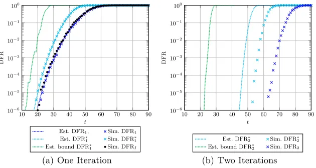
For the case of the decoder performing just one iteration, the simple expression of the DFR has been derived in the proof of Lemma 2, that is
DFR∗1= 1−ProbP∗ n
t−→
1 0
=
Pm|0(t)
n−t t Y
j=1
Pf|1(j).
Actually, for just one iteration, the average DFR (corresponding to the use of a random permutationπ) can be approximated in a very simple way, as follows. Let ai, ai+1, with i ∈ [0;t−2], be two consecutive elements of S (π(e)). Then denote with dthe average zero-run lenght ine, d=E[ai+1−ai] = nt+1−t, ∀i∈ [0;t−2] whereE[·] denotes the expected value. Consequently, we can write
DFR1≈1−
t Y j=1
Pm|0(j)
d t Y l=1
Pf|1(l). (7)
4.2 Simulation Results
10 20 30 40 50 60 70 80 90 10−6
10−5
10−4
10−3
10−2
10−1
100
t
DFR
Est. DFR1, Sim. DFR1
Est. DFR∗
1 Sim. DFR∗1
Est. bound DFR∗
1 Sim. DFRI
(a) One Iteration
10 20 30 40 50 60 70 80 90
10−6
10−5
10−4
10−3
10−2
10−1
100
t
DFR
Est. DFR∗
2 Sim. DFR∗2
Est. bound DFR∗
2 Sim. DFR2
(b) Two Iterations
Fig. 1.Experimental validation of the DFR estimates (Est.) through numerical simu-lations (Sim.). The QC-LDPC code parameters aren0= 2,p= 4,801 andv= 45. The decoding threshold isb0= 25.
each value of the error weight. To this end, we implemented the RIP decoder in C99, and run the experiments on an Intel Core i5-6500 CPU running at 3.20 GHz, compiling the code with the GCC8.3.0 and running the built executables on Debian GNU/Linux 10.2 (stable). The computation of the worst case DFR estimates and bounds in Eq. (2) and Eq. (3) were realized employing the NTL library [24], while the solver for the counting version of the subset sum problem was implemented in plainC++. Computing the entire DFR upper bound relying on the counting subset sum problem takes significantly less than a second, for the selected parameters. We report the results considering a bit flipping threshold of
apply-ing the random permutation to the positions of the error estimates which have randomly-placed discrepancies with the actual error itself.
5
Conclusions
We provided a statistical analysis of the behavior of a randomized in place bit flipping decoder, derived from the canonical one by randomizing the order in which the estimated error positions are processed. This modification to the coder allows us to provide a statistical worst-case analysis of the DFR of the de-coder at hand, both considering the average behavior among all the codes with the same length, dimension and number of parity checks, and a code-specific bound for a given QC-LDPC/QC-MDPC. The former analysis can be fruitfully exploited to design code parameters allowing to obtain DFR values such as the ones needed to employ QC-LDPC/QC-MDPC codes in constructions providing IND-CCA2 guarantees under the assumption that the underlying scheme is δ -correct [14]. The latter result allows us to analyze a given QC-LDPC/QC-MDPC code to assess whether the DFR it exhibits is above the maximum tolerable one for an IND-CCA2 construction, thus allowing us to discard weak keypairs upon generation. We note that our analysis relies on the RIP decoder performing a finite number of iterations, as opposed to the one provided in [23], in turn al-lowing a constant-time implementation of the RIP decoder itself. This fact is of significant practical relevance since the timing information leaked from decoders performing a variable number of iterations was shown to be as valuable as the one leaked by decryption failures to a CCA attacker [9, 22], leading to concrete violations of the IND-CCA2 property.
References
1. G. Agosta, A. Barenghi, G. Pelosi, and M. Scandale. Trace-based schedulability analysis to enhance passive side-channel attack resilience of embedded software.
Inf. Process. Lett., 115(2):292–297, 2015.
2. M. Baldi, A. Barenghi, F. Chiaraluce, G. Pelosi, and P. Santini. LEDAcrypt: QC-LDPC Code-Based Cryptosystems with Bounded Decryption Failure Rate. In M. Baldi, E. Persichetti, and P. Santini, editors, CodeBased Cryptography -7th International Workshop, CBC 2019, Darmstadt, Germany, May 18-19, 2019, Revised Selected Papers, volume 11666 ofLecture Notes in Computer Science, pages 11–43. Springer, 2019.
3. M. Baldi, F. Chiaraluce, R. Garello, and F. Mininni. Quasi-Cyclic Low-Density Parity-Check Codes in the McEliece Cryptosystem. In Proceedings International Conference on Communications (ICC 2007), pages 951–956, Glasgow, Scotland, Jun. 2007.
4. E. R. Berlekamp, R. J. McEliece, and H. C. A. van Tilborg. On the inherent intractability of certain coding problems (Corresp.). IEEE Trans. Information Theory, 24(3):384–386, 1978.
6. N. Bindel, M. Hamburg, K. H¨ovelmanns, A. H¨ulsing, and E. Persichetti. Tighter proofs of CCA security in the quantum random oracle model. Cryptology ePrint Archive, Report 2019/590, 2019. https://eprint.iacr.org/2019/590.
7. T. H. Cormen, C. E. Leiserson, R. L. Rivest, and C. Stein. Introduction to Algo-rithms, Third Edition. The MIT Press, 3rd edition, 2009.
8. N. Drucker and S. Gueron. A toolbox for software optimization of QC-MDPC code-based cryptosystems. Cryptology ePrint Archive, Report 2017/1251, 2017. https://eprint.iacr.org/2017/1251.
9. E. Eaton, M. Lequesne, A. Parent, and N. Sendrier. QC-MDPC: A timing attack and a CCA2 KEM. In T. Lange and R. Steinwandt, editors, PQCrypto, pages 47–76, Fort Lauderdale, FL, USA, Apr. 2018. Springer International Publishing. 10. T. Fabˇsiˇc, V. Hromada, P. Stankovski, P. Zajac, Q. Guo, and T. Johansson. A
Re-action Attack on the QC-LDPC McEliece Cryptosystem. In T. Lange and T. Tak-agi, editors,Post-Quantum Cryptography: 8th International Workshop, PQCrypto 2017, pages 51–68. Springer, Utrecht, The Netherlands, June 2017.
11. J.-C. Faug`ere, A. Otmani, L. Perret, and J.-P. Tillich. Algebraic Cryptanalysis of McEliece Variants with Compact Keys. In H. Gilbert, editor, EUROCRYPT, volume 6110 ofLecture Notes in Computer Science, pages 279–298. Springer, 2010. 12. R. G. Gallager. Low-Density Parity-Check Codes. PhD thesis, M.I.T., 1963. 13. Q. Guo, T. Johansson, and P. Stankovski. A key recovery attack on MDPC with
CCA security using decoding errors. In J. H. Cheon and T. Takagi, editors, ASI-ACRYPT 2016, volume 10031 ofLNCS, pages 789–815. Springer Berlin Heidelberg, 2016.
14. D. Hofheinz, K. H¨ovelmanns, and E. Kiltz. A Modular Analysis of the Fujisaki-Okamoto Transformation. In Y. Kalai and L. Reyzin, editors,Theory of Cryptogra-phy - 15th International Conference, TCC 2017, Baltimore, MD, USA, November 12-15, 2017, Proceedings, Part I, volume 10677 ofLecture Notes in Computer Sci-ence, pages 341–371. Springer, 2017.
15. S. Mangard, E. Oswald, and T. Popp.Power analysis attacks - revealing the secrets of smart cards. Springer, 2007.
16. R. J. McEliece. A public-key cryptosystem based on algebraic coding theory.Deep Space Network Progress Report, 44:114–116, Jan. 1978.
17. R. Misoczki, J.-P. Tillich, N. Sendrier, and P. L. Barreto. MDPC-McEliece: New McEliece variants from moderate density parity-check codes. InProceedings IEEE International Symposium on Information Theory (ISIT 2013), pages 2069–2073, Istambul, Turkey, Jul. 2013.
18. H. Niederreiter. Knapsack-type cryptosystems and algebraic coding theory. Prob-lems of Control and Information Theory, 15(2):159–166, 1986.
19. A. Salomaa. Chapter II - Finite Non-deterministic and Probabilistic Automata. In A. Salomaa, editor,Theory of Automata, volume 100 ofInternational Series of Monographs on Pure and Applied Mathematics, pages 71 – 113. Pergamon, 1969. 20. P. Santini, M. Battaglioni, M. Baldi, and F. Chiaraluce. Hard-Decision Iterative
Decoding of LDPC Codes with Bounded Error Rate. In Proceedings IEEE Inter-national Conference on Communications (ICC 2019), pages 1–6, Shanghai, China, May 2019.
21. P. Santini, M. Battaglioni, M. Baldi, and F. Chiaraluce. A theoretical analysis of the error correction capability of LDPC and MDPC codes under parallel bit-flipping decoding, 2019.
t0= 0 t0= 1 . . . t0=n−t
0,Pf|0(t) 0,Pf|0(t+ 1) 0,Pf|0(n−1)
0,Pm|0(t) 0,Pm|0(t+ 1) 0,Pm|0(n)
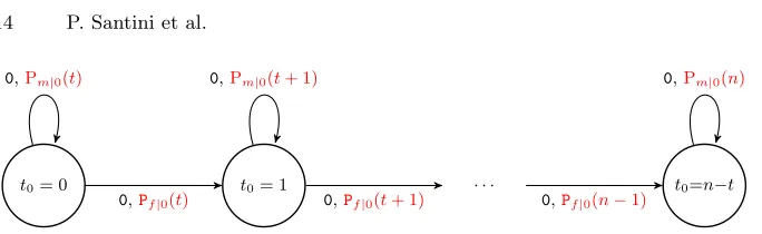
Fig. 2.Structure of the probabilistic FSA modeling the evolution of the distribution of the ˆt0 variable. Read characters are reported in black, transition probabilities in red.
23. N. Sendrier and V. Vasseur. On the Decoding Failure Rate of QC-MDPC Bit-Flipping Decoders. In J. Ding and R. Steinwandt, editors,Post-Quantum Cryptog-raphy - 10th International Conference, PQCrypto 2019, Chongqing, China, May 8-10, 2019 Revised Selected Papers, volume 11505 ofLecture Notes in Computer Science, pages 404–416. Springer, 2019.
24. V. Shoup. NTL: A Library for doing Number Theory. http://shoup.net/ntl/, Version 11.4.1, 2019.
25. J. Tillich. The Decoding Failure Probability of MDPC Codes. In 2018 IEEE International Symposium on Information Theory, ISIT 2018, Vail, CO, USA, June 17-22, 2018, pages 941–945. IEEE, 2018.
A
Deriving the Bit-flipping Probabilities for the RIP
Decoder
Denote with ˆt0 = |{S(e⊕¯e)∩E0}|, that is the number of places where the estimated error at the beginning of the outer loop iteration ¯e differs from the actuale, in positions included inE0. Analogously, define ˆt1=|{S(e⊕¯e)∩E1}|. We now characterize the statistical distribution of ˆt0and ˆt1afterniterations of the inner loop of the RIP-BF decoder are run, processing the estimated error bit positions in the order pointed out by π∗ ∈ P∗
n, i.e., the permutation which places at the end all the positions j where ˆej 6= ej. We point out that, at the first iteration of the outer loop of the decoder, this coincides with placing all the positions whereej= 1 at the end, since ¯eis initialized to then-binary elements zero vector, hence ¯e⊕e=e.
t1= 0 t1= 1 . . . t1=t
1,Pf|1(t∗−t+ 1) 1,Pf|1(t∗−t+ 2) 1,Pf|1(t∗)
1,Pm|1(t∗−t) 1,Pm|1(t∗−t+ 1) 1,Pm|1(t∗)
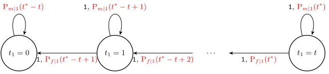
Fig. 3.Structure of the probabilistic FSA modeling the evolution of the distribution of the ˆt1variable. Read characters are reported in black, transition probabilites in
red-We model the statistical distribution of ˆt0as the state of a PFSA havingn−t FSA states, each one mapped onto a specific value for ˆt0, as depicted in Figure 2. We consider the underlying FSA to be accepting the input language constituted by binary strings obtained as the sequences of ˆej 6= ej values, where j is the error estimate position being processed by the RIP decoder at a given inner loop iteration. We therefore have that, for the PFSA modeling the evolution of ˆ
t0while the RIP decoder acts on the firstn−tpositions specified byπ∗, all the read bits will be equal to 0, as π∗ sorts the positions of ˆeso that the (n−t at the first iteration) positions with no discrepancy between ¯eand ecome first.
The transition probability for the PFSA transition from a state ˆt0 = i to ˆ
t0=i+ 1 requires the RIP decoder to flip a bit of ˆeequal to zero, and matching the one in the same position ofe, causing a discrepancy. Because of Assumption 1, the probability of such a transition isPf|0(t+i). , while the probability of the self-loop transition from ˆt0=ito ˆt0=iitself is Pm|0(t+i).
Note that, during the inner loop iterations of the RIP decoder acting on positions of ˆewhich have no discrepancies it is not possible to decrease the value ˆ
t0, as no reduction on the number of discrepancies between ˆeandecan be done changing values of ˆe which are already equal to the ones in e. Hence, we have that the probability of transitioning from ˆt0=ito ˆt0=i−1 is zero.
The evolution of a PFSA can be computed simply taking the current state, represented as the vectoryof probabilities for each FSA state and multiplying it by an appropriate matrix which characterizes the transitions in the PFSA. Such a matrix is derived as the adjacency matrix of the PFSA graph representation, keeping only the edges for which the read character matches the edge label, and substituting the one-values in the adjacency matrix with the probability labelling the corresponding edge. We obtain the transition matrix modeling an iteration of the RIP decoder acting on an ˆej = ej (i.e. reading a 0) as the (n−t+ 1)×(n−t+ 1) matrix:
K0=
Pm|0(t) Pf|0(t) 0 0 0 0
0 Pm|0(t+ 1)Pf|0(t+ 1) 0 0 0 ..
. ... ... ... ... ...
0 0 0 0 Pm|0(n−1)Pf|0(n−1)
0 0 0 0 0 Pm|0(n)
Since we want to compute the effect on the distribution of ˆt0 after n−t iterations of the RIP decoder acting on positions j such that ˆej =ej, we can obtain it simply as yKn0−t. Note that the subsequent t iterations of the RIP decoder will not alter the value of ˆt0 as they act on positionsjsuch thatej= 1. Since we know that, at the beginning of the first iterationy= [Prob ˆt0= 0= 1,Prob ˆt0= 1 = 0,Prob ˆt0= 2= 0,· · ·,Prob ˆt0=n−t= 0], we are able to computeProbP∗
n
ω E0
−−→xas the (x+ 1)-th element ofyKn0−t.
We now model the distribution of ˆt1, during the lasttiterations of the inner loop of the RIP decoder performed during an iteration of the outer loop. Note that, to this end, the first n−t iterations of the inner loop have no effect on ˆ
t1. Denote witht∗ the incorrectly estimated bitswH(e+ ˆe) at the beginning of the inner loop iterations acting on positions j where ˆej6=ej. Note that, at the first iteration of the outer loop of the RIP decoder, t∗ = ˆt0+t, when the RIP decoder is about to analyze the first position for whichwH(e+ ¯e). Arguments analogous to the ones employed to model the PFSA describing the evolution for ˆ
t0allow us to obtain the one modeling the evolution for ˆt1, reported in Figure 3. We are thus able to obtain theProbP∗
n
ω E1
−−→xPFSA reported in Figure 3 for ˆt1 is z = [Prob ˆt1= 0
= 0,Prob ˆt1= 0
= 0, . . . ,Prob ˆt1=t
= 1] and employing the (t+ 1)×(t+ 1) transition matrixK1 of the PFSA to compute
zKt
1. The value ofProbP∗ n
ω E1
−−→x corresponds to the (x+ 1)-th element of
zKt 1.
B
Solving the Counting Subset Sum Problem
In the following, we describe the algorithm computing N(y, η,thr), i.e., the number of subsets of the elements of y, which have cardinality equal toη, and which have the sum of their elements lesser than or equal to thr.
In doing this, we leverage the fact thatyhas only a small number of distinct elements,zn=|y|. To this end, we representyas the sequence of itszdistinct elements [0, 1, . . . , z−1] in increasing order of their value, i.e.,∀i < j, ei < ej. Such a sequence is paired with the sequence of the number of times that eachi appears iny, [λ0, λ1, . . . , λz−1].
First of all, we note that the sets which are counted in N(y, η,thr), can be partitioned according to the number of distinct elements contained in them. Denote withNi(y, η,thr) the number of the number of subsets of the elements of
y, with cardinality equal toη, sum lesser or equal tothr, and exactlyidistinct elements. The value ofN(y, η,thr) is obtained as the sum over alli∈1, . . . , z
of the values of Ni(y, η,thr). The computation of Ni(y, η,thr) is described in Algorithm 2.
C
Proof of Lemma 1
Algorithm 2: Computation ofNi(y, η,thr)
Input: y: an integer sequence, with elements in{0, . . . v},|y|=n. The collection admits repeated items
η: the number of elements of the sought subsets ofy
thr: the maximum allowed value of the sum of theη-wide integer subsets ofy i: the number of distinct elements admitted in the subsets
Output:Ni(y, η,thr): the number of subsets ofy, ofηintegers picked with sum≤thr
Data:z: the number of distinct elements iny
i: thei-th distinct integer iny,i∈ {0, . . . , z−1},i < j⇒i< j
λi: the number of occurrences (multiplicity) ofiiny
1 sum←0
2 ifi= 1then
3 forj←0toz−1do
// Pick η terms equal toj: their sum should be≤thr
4 if (j·η≤thr)∧(λj≥η)then
5 sum←sum+ λiη
6 returnsum
7 else
8 forj←0toz−1do
9 m←min{λj,bthrjc, η−(i−1)}
// i−1 distinct terms must still be placed: place at mostη−(i−1)
10 fork←1tomdo
11 sum←sum+ λjk
N(i−1)(y\ {0. . . j}, η−k,thr−(k·j))
12 returnsum
(0 ≤ z ≤ n−1) is null or not, i.e., Prob(si= 1|ez) = Prob(hhi,:,ei= 1|ez),
hhi,:,ei=L n−1
j=0hi,j·ej, can be expressed for each bit positionz,0≤z≤n−1, of the error vector as follows:
ρ0,u=Prob(hhi,:,ei= 1| ez= 0) =
Pmin{w,t}
l=0,l odd w
l
n−w t−l
n−1 t
ρ1,u=Prob(hhi,:,ei= 1 |ez= 1) =
Pmin{w−1,t−1}
l=0,l even
w−1 l
n−w t−1−l
n−1 t−1
Consequentially, the probability that Algorithm 1 performs a bit-flip of an ele-ment of the estimated error vector, eˆz, when the corresponding bit of the actual error vector is asserted,ez = 1, i.e., Pf|1, and the probability that Algorithm 1 maintains the value of the estimated error vector,ˆez, when the corresponding bit of the actual error vector is null, ez= 0, i.e.,Pm|0, are:
Pf|1= v
X
upc=b
v
upc
ρupc1,u(1−ρ1,u)
v−upc,
Pm|0= b−1
X
upc=0
v
upc
ρupc0,u(1−ρ0,u)
v−upc.
Given a rowhi,:of the parity-check matrixH, such thatz∈S (hi,:), the equation
Ln−1
j=0 hi,j·ej (in the unknowne) yields a non-null value for thei-th bit of the syndrome,si, (i.e., the eq. is unsatisfied) if and only if the support of the error vector eis such thatLn−1
j=0hi,j·ej = 2a+ 1, a≥0, including the term having
j = z, i.e., hi,z·ez = 1. This implies that the cardinality of the set obtained intersecting the support hi,: with the one of e, |(S (hi,:)\ {z})∩(S (e)\ {z})|, must be an even number, which in turn cannot be larger than the minimum between|S (hi,:)\ {i}|=w−1 and|S (e)\ {i}|=t−1.
The probability ρ1,u is obtained considering the fraction of the number of
error vector values having an even number of asserted bits matching the asserted bits ones in a row ofH(noting that, for thez-th bit position, both the error and the row ofHare set) on the number of error vector values havingt−1 asserted bits overn−1 positions, i.e., nt−−11
. The numerator of the said fraction is easily computed as the sum of all error vector configurations having an even number 0 ≤l ≤min{w−1, t−1} of asserted bits. Considering a given value forl, the counting of the error vector values is derived as follows. Picking one of vector withlasserted bits overwpossible positions, i.e., one vector over w−l1
possible ones, there are tn−−1w−l
possible values of the error vector exhibitingt−1−lnull bits in the remainingn−wpositions; therefore, the total number of vectors with weighlis w−l1
· tn−−1w−l
. Repeating the same line of reasoning for each value of
l allows to derive the numerator of the formula definingρ1,u.
From Assumption 2, the value of any rowhi,:is modeled as a random variable with a Bernoulli distribution having parameter (or expected value)ρ1,u, and each
of these random variables is independent from the others. Consequentially, the probability that Algorithm 1 performs a bit-flip of an element of the estimated error vector when the corresponding bit of the actual error vector is asserted and the counter of the unsatisfied parity checks (upc) is above or equal to a given thresholdb, is derived as the binomial probability obtained adding the outcomes ofv (column-weight ofH) i.i.d. Bernoulli trials. ut
D
Proof of Lemma 2
Lemma 2. The execution path of the inner loop in Algorithm 1 yielding the worst possible decoder success rate is the one taking place when π∗ ∈ P∗
n is applied at the beginning of the outer loop, that is:
∀π∈ Pn,∀π∗∈ Pn∗, Prob( ˆe6=e| π∈ Pn)≤Prob( ˆe6=e| π
∗∈ P∗
n). Proof. First of all, we can writeProb(e0 6=e| π∈ P
n) = 1−β(π),whereβ(π) is the probability that all bits, evaluated in the order specified byπ, are correctly processed. To visualize the effect of a permutationπ∗∈ Pn, we can consider the following representation
π∗(e)⊕π∗(¯e) = [0,0,· · ·,0
| {z }
lengthn−ˆt
,1,1,· · ·,1
| {z }
length ˆt
The decoder will hence analyze first a run ofn−ˆtpositions where the differences between the permuted errorπ∗(e) vector andπ∗(¯e) contain only zeroes, followed by a run of ˆtpositions containing only ones. Thus, we have that
β(π∗) = Pm|0(ˆt)
n−ˆt
·Pf|1(ˆt)·Pf|1(ˆt−1)· · ·Pf|1(1)
The former expression can be derived thanks to Assumption 1 as follows. Note that, the first elements in the first n−ˆt positions of π∗(ˆe) and π∗(e) match,
therefore the decoder makes a correct evaluation if it does not change the value ofπ∗(ˆe). This in turn implies that, in case a sequence ofn−ˆtcorrect decisions are made in the corresponding iterations of the inner loop, each iteration will have the same probability Pm|0(ˆt) correctly evaluating the current estimated error bit. This leads to a probability of performing the first n−tˆiterations taking a correct decision equal to Pm|0(ˆt)
n−ˆt
Through an analogous line of reasoning, observe that the decoder will need to change the value of the current estimated error bit during the last ˆt iterations of the inner loop. As a consequence, if all correct decisions are made, the number of residual errors will decrease by one at each inner loop iteration, yielding the remaining part of the expression.
Consider now a generic permutation π, such that the resulting π(e) has support{u0,· · ·, uˆt−1}; we have
β(π) =
Pm|0(ˆt) u0
Pf|1(t)
Pm|0(ˆt−1)
u1−u0−1
Pf|1(ˆt−1)· · ·Pf|1(1)
Pm|0(0)
n−1−utˆ−1
=
Pm|0(t) u0
Pm|0(0)
n−1−uˆt−1
ˆ t−1 Y
j=1
Pm|0(ˆt−j)
uj−uj−1−1
ˆ t−1 Y
l=0
Pf|1(ˆt−l).
We now show that we always haveβ(π)≥β(π∗). Indeed, since Pm|0(0) = 1 and due to the monotonic trends of Pu and Pf, the following chain of inequalities can be derived
β(π) =
Pm|0(0)
n−1−uˆt−1
Pm|0(ˆt) u0
ˆ t−1 Y
j=1
Pm|0(ˆt−j)
uj−uj−1−1
ˆ t−1 Y
l=0
Pf|1(ˆt−l)
≥
Pm|0(0)
n−1−uˆt−1
Pm|0(ˆt) u0
ˆ t−1 Y
j=1
Pm|0(ˆt)
uj−uj−1−1
ˆ t−1 Y
l=0
Pf|1(ˆt−l)
=
Pm|0(0)
n−1−uˆt−1
Pm|0(ˆt) u0
Pm|0(ˆt)
utˆ−1−u0−(ˆt−1)
ˆ t−1 Y
l=0
Pf|1(ˆt−l))
=
Pm|0(0)
n−1−uˆt−1
Pm|0(ˆt)
uˆt−1−(ˆt−1)
ˆ t−1 Y
l=0
Pf|1(ˆt−l)
≥
Pm|0(ˆt)
n−1−uˆt−1
Pm|0(ˆt)
uˆt−1−(ˆt−1)
ˆ t−1 Y
l=0
Pf|1(ˆt−l)
=
Pm|0(ˆt) n−ˆt
ˆ t−1 Y
l=0
Pf|1(ˆt−l) =β(π ∗
).