The secrets of profiling for side-channel analysis: feature selection matters

(1)

feature selection matters

Stjepan Picek1_{, Annelie Heuser}2_{, Alan Jovic}3_{, Lejla Batina}4_{, Axel Legay}5 1

Delft University of Technology, The Netherlands

2

CNRS, IRISA, Rennes, France

3 _{University of Zagreb, Croatia} 4

Radboud University, Digital Security, Nijmegen, The Netherlands

5 _{Inria, IRISA, Rennes, France}

Abstract. Profiled side-channel attacks feature a number of steps one needs to take. One significant step, importance of which is sometimes ignored, is selection of the points of interest (features) within side-channel measurement traces. A large majority of the related works on profiling in side-channel analysis starts with an assumption that the features are somehow selected and distinct attack methods are compared in order to find the best approach for the key recovery.

Contrary to this, in this work we concentrate on the feature selection step and show that if an optimal selection is done, most of the attack techniques perform well i.e., result in the key recovery. Consequently, in this paper, we investigate in details how more advanced feature selection techniques stemming from the machine learning domain can be used to improve the attack efficiency. To this end, we look into relevant aspects and we provide a systematic evaluation of machine learning methods of interest.

Our results show that the so-called Hybrid feature selection methods per-form with the best classification accuracy over a wide range of test scenar-ios and number of features selected. The experiments are performed on several real-world data sets containing software and hardware implemen-tations of AES, and even including the random delay countermeasure. We emphasize the L1 regularization technique, which consistently performed well and in many cases resulted in significantly higher accuracy than the second best technique. Further on, we consider even Principal Compo-nent Analysis (PCA) as a typical dimensionality reduction method and show that feature selection combined with the ML classification remains the method of choice (when confronted with PCA).

1 Introduction

(2)

analysis can be extremely powerful for key recovery, with machine learning being a highly viable choice.

Contrary, feature selection, and in particular the usage of ML based tech-niques, did not receive a significant attention. Early works on template attacks introduced SOST/SOSD [5] as feature selection methods and consequently most of the follow-up works assume that this step has somehow been performed in a satisfactory, if not optimal manner. A common strategy often also suggests using Pearson correlation for this purpose e.g., [1, 2, 6].

There are a number of papers considering profiled SCA, where the number of features is fixed and the analysis is conducted by considering only the changes in the number of traces or by selecting a more powerful classifier, see e.g., [7–9]. In this work, we take those observations one step further. We show not only that feature selection is a crucial step in profiling attacks but we also shed some light on how to use it for the following goals:

– training a model faster,

– reducing the complexity of a model,

– improving the accuracy of a model (when suitable features are selected), – reducing overfitting,

– “correcting” the covariance matrix in template attack when the number of features is too large with respect to the number of traces.

It is somewhat surprising that the SCA community (until now) did not take a closer look into the feature selection part of the classification process. Simi-lar to the powerful classification methods coming from the ML domain, there are also other feature selection techniques one could utilize. To the best of our knowledge, there exists merely one work that is focusing on the feature selec-tion for profiled SCA [10] but it does not consider machine learning techniques and it compares only methods known for side-channel analysis either as feature selection techniques or distinguishers.

Note that, in leakage detection (see e.g., [11]), one is identifying data-dependent but not necessarily model-agnostic leakage information. Consequently, detecting features (points in the trace) is somehow a task orthogonal to leakage detec-tion as leakage detecdetec-tion (according to e.g., TVLA) may not necessarily lead to a successful key recovery. However, one approach could be as follows: first use leakage detection to identify possible leakages in the trace, then analyze the corresponding operation, in particular, determine if the model is key sensitive, and finally use feature selection in combination with the underlying model for a profiled distinguisher. In this paper, we purely concentrate on feature selection techniques.

More precisely, we investigate how the efficiency of SCA distinguishers can in-crease due to feature selection techniques. When discussing features (also known as points of interest, points in time, variables, attributes), we can distinguish among relevant, irrelevant, and redundant features. A meaningful separation of those is very important in optimizing the attack strategy.

(3)

this, we employ a number of feature selection techniques ranging from “simple” ones like the Pearson correlation, which is de-facto standard in the side-channel community, to more complex approaches such as various Wrapper and Hybrid methods used in the ML domain. To the best of our knowledge, such advanced techniques have never been used in the context of SCA before. We summarize our contributions in more detail below.

1.1 Our contributions

Our main contributions are as follows:

1. We introduce a novel approach of using ML techniques for the important problem of feature selection in SCA.

2. We demonstrate the potential of Wrapper and Hybrid methods in SCA as they perform the best for feature selection on the examined datasets. 3. We show how to overcome some previously identified shortcomings of

tem-plate attacks by the ML techniques, which not just solves the problems but improves upon the accuracy of templates as well.

4. Our methods also turn out to lead to the dimensionality reduction when supported with a “proper” designation of a feature selection subset. This suggests that selected classifiers can be also viable competitors for PCA-like techniques for dimensionality reduction.

5. All our results are verified on the real-world data sets i.e., two AES imple-mentations from the DPA contest (software and hardware) and one AES implementation on an 8-bit microcontroller with random delays as a coun-termeasure.

1.2 Previous work

Ever since the seminal work of Chari et al. introducing template attacks [12], efforts were put into optimizing those and enlarging their scope. The observation on the profiling, i.e., training phase in template attacks, has naturally led to machine learning techniques and their potential impact on the key recovery phase.

(4)

To the feature selection problem, there were very few attempts and works devoted, as some simple techniques were considered satisfactory enough. For ex-ample, early works that introduced SOST/SOSD [5] as feature selection meth-ods and consequently the majority of follow-up papers skipped this step com-pletely. One strategy also suggested using Pearson correlation for this purpose e.g., [1, 2, 6], which is an obvious solution but does not answer the following question: can we do better?

Some authors noticed the importance of finding adequate time points in other scenarios. Reparaz et al. [14] introduced a novel technique to identify such tuples of time samples before key recovery for multivariate DPA attacks. A typical use case that the attacker is confronted with in this case is a masked implementation, requiring higher-order attacks (and hence multiple features corresponding to the right time moments e.g. when mask is generated and manipulated).

Zheng et al. looked into this specific feature selection question but left ML techniques aside [10]. Picek et al. considered a number of machine learning tech-niques for profiling attacks and investigated the influence of the number of fea-tures in the process by applying Information Gain feature selection [15]. Thus, our work is the first one to address feature selection problematics from the ML perspective in details. Finally, we also question the previous results on dimen-sionality reduction as our comparison of ML feature selection and PCA (which is feature extraction) favors the former.

This paper is organized as follows. In Sect. 2, we introduce our notation and we also describe the datasets used in experiments. Sect. 3 reminds a reader on template attacks and reviews machine learning algorithms of interest for profiling. Sect. 4 explains feature selection techniques that are used in the rest of the paper. Sect. 5 presents our results and gives a discussion on the relevance of our findings. Sect. 6 points to several directions for possible future work and concludes the paper.

2 Background

2.1 Our notation

Calligraphic letters (e.g.,X) denote sets, capital letters (e.g.,X) denote random variables taking values in these sets, and the corresponding lowercase letters (e.g., x) denote their realizations. Letk∗ be the fixed secret cryptographic key (byte) and the random variableTthe plaintext or ciphertext of the cryptographic algorithm which is uniformly chosen. The measured leakage is denoted asX and we are particularly interested in multivariate leakage X =X1, . . . , XD, where

D is the number of time samples or features (attributes) in machine learning terminology.

(5)

(i.e., it has dimension D×N). In the attack phase, the attacker then measures additional traces X1, . . . ,XQ from the device under attack in order to break the unknown secret keyk∗.

2.2 Datasets

In our experiments, we use three data sets as outlined below.

DPAcontest v2 [16] DPAcontest v2 provides measurements of an AES hard-ware implementation. Previous works showed that the most suitable leakage model (when attacking the last round of an unprotected hardware implementa-tion) is the register writing in the last round, i.e.,

Y(k∗) = Sbox−1[Cb1⊕k

∗_]

| {z }

previous register value

⊕ Cb2 |{z} ciphertext byte

, (1)

where Cb1 and Cb2 are two ciphertext bytes, and the relation between b1 and

b2 is given through the inverse ShiftRows operation of AES. In particular, we

choose b1 = 12 resulting in b2 = 8 as it is one of the easiest bytes to attack6.

In Eq. (1),Y(k∗_{) consists of 256 values, as an additional model we applied the} HW on this value resulting in 9 classes. These measurements are relatively noisy and the resulting model-based SNR (signal-to-noise ratio), i.e., var_var(₍signal_noise₎) =

var(y(t,k∗))

var(x−y(t,k∗₎₎,with a maximum value of 0.0096. We conduct our experiments by starting with the whole AES trace consisting of 3 253 features.

DPAcontest v4 [17] The 4th version provides measurements of a masked AES software implementation. As the mask is known, one can easily turn it into an unprotected scenario. As it is a software implementation, the most leaking operation is not the register writing but the processing of the S-box operation and we attack the first round. Accordingly, the leakage model changes to

Y(k∗) =Sbox[Pb1⊕k

∗_]_⊕ _M

|{z} known mask

, (2)

where Pb1 is a plaintext byte and we choose b1= 1. Compared to the

measure-ments from version 2, the SNR is much higher with a maximum value of 5.8577. For our experiments, we start with a preselected window of 4 000 features from the original trace (we preselect all features around the S-box operation).

Random Delay Countermeasure [18] As our third use case, we use an actual protected implementation to prove the potential of our approach. Our target is a software implementation of AES on an 8-bit Atmel AVR microcontroller with

6

(6)

implemented random delay countermeasure as described by Coron and Kyzhva-tov in [18]. We mounted our attacks in the Hamming weight power consumption model against the first AES key byte, targeting the first S-box operation. The data set consists of 50 000 traces of 3 500 features each. For this dataset, the SNR has a maximum value of 0.0556.

3 Profiled Attacks

In this section, we introduce the methods we use in the classification tasks. Note that we opted to work with only a small set of techniques, since we aim to ex-plore how to find the best possible subset of features, while the classification task should be considered as just a means of comparison among feature selec-tion methods. Consequently, we try to be as “method-agnostic” as possible and we note that for each set of features, one could probably find a classification algorithm performing slightly better.

3.1 Naive Bayes

The Naive Bayes classifier is a method based on the Bayesian rule, which works under a simplifying assumption that the predictor features (measurements) are mutually independent among theDfeatures, given the class valueY. Existence of highly-correlated features in a dataset can thus influence the learning process and reduce the number of successful predictions. Additionally, Naive Bayes assumes s normal distribution for predictor features. A Naive Bayes classifier outputs posterior probabilities as a result of the classification procedure [19].

The space complexity for Naive Bayes algorithm for both training and testing phase is O |Y|Dv, where |Y| is the number of classes, D is the number of features, andvis the average number of values for a feature. The time complexity for the training phase equals O N D and for the testing phase it is equal to O |Y|D

, withN being the number of training examples.

3.2 Support Vector Machines

Support Vector Machine (SVM) is a kernel based machine learning family of methods that are used to accurately classify both linearly separable and linearly inseparable data [20]. The SVM algorithm is parametric and deterministic. The basic idea when the data are not linearly separable is to transform them to a higher dimensional space by using a transformation kernel function. In this new space, the samples can usually be classified with a higher accuracy. For classification purposes, we use radial-based SVM, where the most significant parameters are the cost of the marginC and the radial kernel parameterγ. A lowC makes the decision surface smooth, while a highC aims at classifying all training examples correctly. The parameterγdefines how much influence a single training example has where the larger γ is, the closer other examples must be to be affected. The time complexity for SVM with radial kernel is O DN3

(7)

the space complexity is O DN2

. For feature selection purposes, we use linear SVM as Wrapper method, because the evaluation is significantly faster (in time and space complexity range of O DN

) than radial-based SVM. We note that utilizing a linear kernel is an efficient choice when the number of dimensions is high (as in our case) or when we can assume there is a linear separation between data.

3.3 Template Attack

Similar to the Naive Bayes classifier, the template attack relies on the Bayes the-orem but considers the features as dependent. In the state-of-the art, template attack relies mostly on a normal distribution. Accordingly, template attack as-sumes that eachP(X =x|Y =y) follows a (multivariate) Gaussian distribution that is parameterized by its mean and covariance matrix for each class Y. The authors of [21] propose to use only one pooled covariance matrix averaged over all classesY to cope with statistical difficulties and thus a lower efficiency. Besides the standard approach, we additionally use this version of the template attack in our experiments. The time complexity for TA is O N D2in the training phase and O |Y|D2

in the testing phase, while the space complexity is O |Y|D2_v

.

4 Feature Selection Techniques

When considering how to select the most important features, i.e., when deal-ing with the feature subset selection problem, an algorithm must find a way of selecting some subset of features, while ignoring the rest of them. Such an algo-rithm can be classified into three broad classes of feature selection techniques: Filter methods, Wrapper methods, and Hybrid methods [22]. Note that, the first three presented Filter methods have been used as feature selection techniques for side-channel analysis in previous works, whereas the remaining methods to our best knowledge, have never been studied to find features in traces.

4.1 Filter Selection Methods

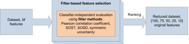
The selection of features with Filter methods is independent of the classifier method. Features are selected on the basis of their scores obtained after running various types of statistical tests. We give a depiction of Filter methods principle in Figure 1, with methods and numbers pertaining to our work.

Pearson Correlation Coefficient Pearson correlation coefficient measures linear dependence between two variables,xandy, in the range [−1,1], where 1 is total positive linear correlation, 0 is no linear correlation, and−1 is total negative linear correlation. Pearson correlation for a sample of the entire population is defined by [23]:

P earson(x, y) =

PN

i=1((xi−x¯)(yi−y¯))

q PN

i=1(xi−x¯)2

q PN

i=1(yi−y¯)2

(8)

Fig. 1: Filter methods

It should be mentioned that Pearson correlation was calculated in our case for the target class variables HW and intermediate value, which consists of categor-ical values that are interpreted as numercategor-ical values. The features are ranked in descending order of Pearson correlation coefficient.

SOSD In [5], the authors proposed as a selection method the sum of squared differences, simply as:

SOSD(x, y) = X i,j>i

(¯xyi−x¯yj)

2_, ₍₄₎

where ¯xyi is the mean of the traces where the model equalsyi. Because of the square, SOSD is always positive. Another advantage of using the square is to enlarge big differences.

SOST SOST is the normalized version of SOSD [5] and is thus equivalent by the pairwise student T-test:

SOST(x, y) = X i,j>i

(¯xyi−x¯yj)/

s

σ2

yi

nyi +σ

2

yj

nyj

!2

(5)

with nyi and nyj being the number of traces where the model equals toyi and

yj, respectively.

Symmetric Uncertainty Symmetric Uncertainty (SU) ranks the quality of a feature using the expression [24]:

SU(X, Y) = 2H(X)−H(X|Y)

(9)

4.2 Wrapper Selection Methods

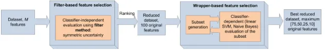
In Wrapper methods [26], there is a feature selection algorithm implemented as a wrapper around a classifier. The feature selection algorithm conducts a search for a good subset by using the classifier algorithm as a part of the function evaluating feature subsets, as depicted in Figure 2. Note that in the Wrapper techniques, the classifier algorithm is considered as a black box. The classifier is run on the dataset with different sets of features removed from the data. The subset of features with the highest evaluation is chosen as the final set on which to run the classifier [27].

Fig. 2: Wrapper methods

More precisely, we use “best-first” forward direction search method to find feature subsets. This strategy uses greedy hill climbing with backtracking capa-bilities, starting from an empty feature subset and inspecting how the addition of a feature to the set influences the output of the classifier. The feature that increases the accuracy the most is kept in the selected set. When backtracking to a smaller set and examining all such paths through the feature set does not lead to better results, the search ends. The search may backtrack to at mostkearlier branching decisions, which is a parameter of the search. Although the overall worst case time and space complexity of the search is exponential in the number of branching decisions kgiven a set of features D, i.e., O Dk

, the complexity is reduced by keeping ksmall.

For our experiments, we use two different classifiers in combination with wrapper selection techniques. First, the Naive Bayes classifier as explained in Section 3.1 [28, 29] and, second, SVM with a linear kernel. The details on SVM are given in Section 3.2. Note that, since wrapper methods check a number of different subsets, the feature selection process is often treated as a high-dimensional problem.

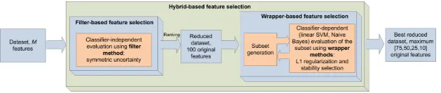
4.3 Hybrid Selection Methods

(10)

Fig. 3: Hybrid methods

L1-based Feature Selection In general, regularization encompasses methods that add a penalty term to the model, which then in turn reduces the overfitting and improves generalizations. L1 regularization works by adding a regularization term α·R(θ), where θ represents the parameters of the model that is used to penalize large weights/parameters. For anD-dimensional input (i.e., the number of features equal toD),R(θ) is equal toPD

i=1|θi|. In the regularization term,α

controls the trade-off between fitting the data and having small parameters. By adding a penalty for each non-zero coefficient, the expression forces weak features to have zero as coefficients, where a zero value means that the feature is omitted from the set. The usage of L1 regularization as a tool for feature selection is well known, for example the linear least-squares regression with L1 regularization (Lasso) algorithm [30]. There can be certain effects with L1 regularization when used for feature selection: most notably, out of a group of highly correlated features, L1 regularization will tend to select an individual feature [31]. In all our experiments, we use linear SVM with L1 for hybrid feature selection.

Stability Selection Stability selection is a method based on subsampling in combination with some classification algorithm (that can work with high-dimensional data) [32]. The key concept of stability selection is the stability paths, which is the probability for each feature to be selected when randomly resampling from the data. In other words, a subsample of the data is fitted to the L1 regularization model, where the penalty of a random subset of coefficients has been scaled. By repeating this procedure n times, the method will assign high scores to the features that are repeatedly selected.

We use multinomial logistic regression for this task and we set the number of randomized models to 5. Multinomial logistic regression uses a linear predictor function f(k, i) to predict the probability that observation i has the outcome

k, of the form f(k, i) = β0,k+β1,kx1,i+. . .+βM,kxM,i where βM,kxM,i is a regression coefficient of themth variable and thekth outcome. Theβcoefficients are estimated using the maximum likelihood estimation, which requires finding a set of parameters for which the probability of the observed data is the greatest.

5 Experimental Evaluation

(11)

of features that is sufficient to learn the mapping from the features X to the classes Y. Since our datasets have a very large number of features, we divide our experiments into two phases. The first phase concentrates on reducing the number of features to the smaller subsets of sizes [10,25,50,75,100] with the Filter methods, i.e., using Pearson correlation, SOSD, SOST, and Symmetric Uncertainty. Once we select the 100 most important features by utilizing those methods, then we additionally use more computationally intensive techniques (two based on the Wrapper techniques, and two based on Hybrid methods) to find smaller subsets (see Section 4). Note that we use Symmetric Uncertainty as the source from where to reduce features with the Wrapper and Hybrid methods. Instead of the Symmetric Uncertainty, any other technique could have been chosen; we opted to use it due to its stability and high performance over all datasets and models.

From the initial datasets, we randomly select 15 000 traces for each one. We divide them in 2:1 ratio where we take the bigger set as the training set (10 000 traces) and the smaller set for testing (5 000 traces). On the training set, we conduct a 5-fold cross-validation and use the averaged results of individual folds to select the best classifier parameters. Note that we report results from the testing phase only where we present them as the accuracy (%) of the classifier, where the accuracy is the number of correctly classified traces divided by the total number of traces. Note that for the intermediate model, Naive Bayes is used instead of radial based SVM as ML classifier, since radial based SVM is computationally more complex to conduct (as we have 256 classes instead of 9) and our focus lies on the feature selection techniques. All experiments are done with MATLAB, Python, and Weka tools [33].

For SVM with radial kernel that is used for final classification purposes, we conduct tuning of the margin C and the radial kernel parameter γ. For the C

parameter we explore values in range [0.01,0.1,1,2,5,10,20,30,40,50,60] and forγ in

[0.01,0.02,0.05,0.1,0.2,0.3,0.4,0.5,0.6,1.0] range. For the DPAcontest v4, we select as the best parameter combination γ= 0.4 and C = 5. For DPAcontest v2, we useγ= 0.05 andC= 2. For all investigated Wrapper methods, we allow at mostk= 5 earlier branching decisions.

When using the linear SVM as Wrapper, we tune the parameter C in the range [0.01,0.02,0.05,0.1,0.5,1,5] and we select it to be equal to 1 for all datasets. Finally, for the L1 regularization with the linear SVM, we again tune the pa-rameterCin the range [0.01,0.02,0.05,0.1,0.5,1,5] and we select the parameter

C to be equal to 0.01.

(12)

Fig. 4: SOST and Symmetric Uncertainty results for DPAcontest v4, HW model

Hybrid methods, selecting the exact number of features can be difficult (since the methods can simply discard multiple features) and consequently subset sizes of [10,25,50,75] represent an upper bound on the number of actually selected features.

5.1 DPAcontest v4

Tables 1 and 2 display the results for DPAcontest v4 with the HW model (i.e.,

HW(Y(k∗_{))) and intermediate value model (i.e.,}_Y₍_k∗_{)), respectively. For each} size of the feature subset, we give the best obtained solution in a cell with gray background color.

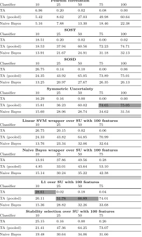
When considering the HW model, we observe that Symmetric Uncertainty is the best option when having 100 features, closely followed by SOSD and SOST. Naturally, for a subset containing 100 features, we do not expect significant dif-ference between the techniques, as it is very likely that all techniques select a very similar subset and even minor differences will not influence the accuracy highly. Still, Table 1 shows weaker results with Pearson correlation compared to other methods. For smaller numbers of features, we observe that the Hybrid methods are performing the best. Interestingly, taking 75 features with L1 regu-larization is nearly as accurate as taking 100 features with SOST and therefore one can reduce the complexity of the attack by considering a more advanced fea-ture selection technique as preprocessing. Also, we cannot conclude that SOST is always superior to SOSD as stated in previous works but is better in the majority of cases.

(13)

Table 1: Accuracy for DPAcontest v4 - HW model

Pearson correlation

Classifier 10 25 50 75 100

TA 57.66 59.38 10.72 5.14 0.14

TA (pooled) 55.18 55.98 81.73 83.77 88.88

SVM 59.44 66.10 80.90 90.92 94.89

SOST

Classifier 10 25 50 75 100

TA 72.63 76.61 0.80 15.97 0.00

TA (pooled) 70.19 73.49 81.35 88.06 92.30

SVM 74.55 80.95 93.11 95.26 96.37

SOSD

Classifier 10 25 50 75 100

TA 73.15 76.99 28.23 1.04 33.25

TA (pooled) 70.05 74.79 77.57 85.21 90.30

SVM 74.71 82.63 88.79 93.98 95.99

Symmetric Uncertainty

Classifier 10 25 50 75 100

TA 72.19 73.35 19.23 62.62 0.76

TA (pooled) 69.87 70.39 81.09 83.77 91.30

SVM 73.32 81.60 93.14 95.32 97.54

Linear SVM wrapper over SU with 100 features

Classifier 10 25 50 75

TA 73.29 83.03 8.64 4.62

TA (pooled) 69.99 82.01 88.98 89.54

SVM 74.26 90.02 95.84 96.70

Naive Bayes wrapper over SU with 100 features

TA 71.65 72.71 76.27 70.53

TA (pooled) 70.17 69.57 73.97 68.33

SVM 73.48 74.78 80.38 74.86

L1 over SU with 100 features

TA 72.19 76.93 24.89 0.86

TA (pooled) 69.87 74.37 82.17 90.58

SVM 83.92 90.28 95.16 97.08

Stability selection over SU with 100 features

TA 72.19 72.81 6.60 4.42

TA (pooled) 69.87 71.23 80.95 90.88

SVM 74.22 92.04 95.78 96.90

(14)

at-Table 2: Accuracy for DPAcontest v4 - intermediate value model

Pearson correlation

Classifier 10 25 50 75 100

TA 6.96 0.20 0.02 0.08 0.00

TA (pooled) 5.42 8.62 27.03 49.98 60.64

Naive Bayes 5.16 7.88 13.30 18.46 22.38

SOST

Classifier 10 25 50 75 100

TA 18.51 0.20 0.02 0.00 0.02

TA (pooled) 18.53 37.94 60.56 72.23 74.71

Naive Bayes 13.91 21.67 24.91 31.18 32.13

SOSD

Classifier 10 25 50 75 100

TA 26.75 0.14 0.10 0.00 0.06

TA (pooled) 24.35 43.92 65.05 73.89 75.01

Naive Bayes 13.25 20.97 27.67 26.35 26.13

Classifier 10 25 50 75 100

TA 16.29 0.16 0.00 0.00 0.00

TA (pooled) 15.81 36.23 60.02 74.65 75.05

Naive Bayes 15.60 28.96 28.74 34.62 31.54

TA 26.75 20.15 0.02 0.06

TA (pooled) 24.33 43.82 64.85 70.99

Naive Bayes 13.76 23.34 32.06 32.64

TA 13.91 37.86 49.56 0.28

TA (pooled) 4.85 33.01 43.64 53.10

Naive Bayes 15.14 30.24 35.22 42.38

TA 28.61 0.02 0.18 0.04

TA (pooled) 26.11 51.78 66.89 74.01

Naive Bayes 15.36 28.82 32.26 33.68

TA 25.15 0.16 0.00 0.26

TA (pooled) 21.41 47.36 64.25 73.07

Naive Bayes 19.48 30.64 34.06 31.66

(15)

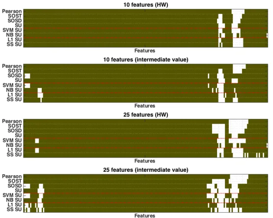
no-Fig. 5: Selected features (in white) over the complete preselected window of 4 000 features from the original trace (DPAcontest v4). SVM SU denotes Support Vector Machine Wrapper, NB SU denotes Naive Bayes Wrapper, L1 SU denotes L1-based Feature Selection, and SS SU denotes Stability Selection.

tice that when using more than approximately 45 features, the accuracy is not stable anymore, which stems from an imprecise estimation of the covariance ma-trices. More precisely, as we consider the HW model, the amount of traces within one class follows a binomial distribution, and thus HW classes 0 and 8 contain much less traces than the other HW classes. Now, as the estimation becomes unstable, in the testing phase TA classifies the traces to classes with unstable covariance matrices, which naturally results in low accuracies. Interestingly, the Naive Bayes wrapper removes the features such that it becomes more efficient than the pooled TA. So, instead of using only one pooled covariance matrix, which reduces the precision for each class, we show that good feature selection can also help with instabilities and even give higher accuracies.

When using the intermediate value model (see Table 2), we observe that, for a larger number of features, Symmetric Uncertainty is the best choice, while for the smaller number of features, L1 regularization is by far the best. From Tables 1 and 2 we notice the obtained accuracies may differ significantly, which is to be expected due to the different models but the question is what are the different selected features.

(16)

Fig. 6: Zoom in into Figure 5 (region with the most selected features)

For the subset of 10 features, one can notice that the area is approximately the same over all techniques. Interestingly, all techniques, except Pearson correla-tion, SOST, and SU, select an additional area for the intermediate value model compared to the HW model. When looking at the subset of 25 for the HW model, we observe that, indeed, stability selection, which results in the highest accuracy for SVM using 25 features, is selecting an additional area of features that is not selected by the other methods. For the intermediate value model, in which L1 over SU is the best technique, we can make the same observation.

To take a look at this behavior in more detail, we depict Figure 5 and addi-tionally Figure 6, which represents a zoom of the interesting area. First, even if the broad area for the subset of 10 features is the same, each technique selects distinct individual features. Finally, our previous observations about the best performing techniques for a subset of 10 and 25 features for both models are confirmed in Figure 6.

5.2 DPAcontest v2

(17)

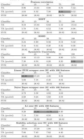
Table 3: Accuracy for DPAcontest v2 - HW model

Pearson correlation

Classifier 10 25 50 75 100

TA 9.96 15.61 0.86 6.76 7.12

TA (pooled) 4.64 6.32 7.30 9.16 9.12

SVM 26.80 26.82 26.82 26.78 26.92

SOST

Classifier 10 25 50 75 100

TA 9.18 15.85 6.02 1.12 15.41

TA (pooled) 5.78 5.84 6.52 7.88 8.08

SVM 26.82 26.82 26.82 26.82 26.82

SOSD

Classifier 10 25 50 75 100

TA 0.24 0.40 0.32 0.54 0.42

TA (pooled) 0.44 0.44 0.46 0.42 0.40

SVM 26.82 26.82 26.82 26.82 26.82

Classifier 10 25 50 75 100

TA 9.80 15.13 9.06 8.90 3.74

TA (pooled) 7.36 8.50 8.20 8.20 9.28

SVM 26.82 26.82 26.82 26.82 26.82

TA 10.80 15.23 4.26 3.82

TA (pooled) 5.66 7.18 8.40 8.84

SVM 26.82 26.82 26.82 26.82

TA 2.72 3.38 4.92 2.62

TA (pooled) 2.68 3.24 5.92 3.58

SVM 26.82 26.82 26.82 26.82

TA 9.28 15.81 11.78 0.40

TA (pooled) 7.18 7.50 8.50 9.14

SVM 26.82 26.82 26.82 26.82

TA 10.64 15.29 1.90 1.42

TA (pooled) 7.66 7.40 7.82 8.40

SVM 26.82 26.82 26.82 26.82

(18)

Table 4: Accuracy for DPAcontest v2 - intermediate value model

Pearson correlation

Classifier 10 25 50 75 100

TA 0.28 0.34 0.40 0.34 0.40

TA (pooled) 0.38 0.52 0.34 0.32 0.38

Naive Bayes 0.50 0.46 0.38 0.40 0.44

SOST

Classifier 10 25 50 75 100

TA 0.24 0.40 0.32 0.54 0.42

TA (pooled) 0.44 0.44 0.46 0.42 0.40

Naive Bayes 0.46 0.50 0.46 0.5 0.54

SOSD

Classifier 10 25 50 75 100

TA 0.36 0.20 0.36 0.38 0.48

TA (pooled) 0.52 0.40 0.44 0.40 0.52

Naive Bayes 0.52 0.48 0.46 0.48 0.50

Classifier 10 25 50 75 100

TA 0.34 0.44 0.46 0.50 0.44

TA (pooled) 0.34 0.34 0.38 0.36 0.36

Naive Bayes 0.50 0.50 0.40 0.58 0.46

TA 0.36 0.36 0.36 0.44

TA (pooled) 0.32 0.52 0.38 0.40

Naive Bayes 0.38 0.42 0.42 0.46

TA 0.50 0.60 0.40 0.40

TA (pooled) 0.48 0.56 0.56 0.56

Naive Bayes 0.32 0.52 0.66 0.66

TA 7.08 27.27 0.00 0.00

TA (pooled) 1.50 3.22 5.48 9.70

Naive Bayes 0.36 0.58 0.50 0.40

TA 5.54 0.00 0.00 0.00

TA (pooled) 1.60 2.70 5.86 8.82

Naive Bayes 0.48 0.46 0.54 0.58

(19)

Fig. 7: Features selected in the last round of AES (DPAcontest v2)

respect to the accuracy, the most effective principle is to put most of the records into the HW class 4. However, clearly, this will not be beneficial in SCA setting. When only looking at TA and TA pooled methods, we observe that the Pearson correlation reaches the best solution for a subset of 75 features, which is only slightly higher than L1 over SU. For 100 features, SU results in the highest accuracy, for 10 features SVM wrapper over SU performs the best, and L1 over SU performs the best for 25 and 50 features.

When considering the intermediate value model, Table 4 shows that L1 over SU finds the best feature subsets for 10, 25, and 75 features. The other Hybrid method, SS over SU find the best result for 50 features, and finally, for 100 features SOST reaches the highest accuracy. We note that, in this scenario, the classification is relatively complex and accuracies are very low (and in some cases also random). So, again as for DPAcontest v4, we observe that Hybrid techniques (in particular L1 over SU) perform effectively as a feature selection method for the HW as well as the intermediate value model.

The selected features over the computation of the last round of AES is dis-played in Figure 7. Compared to the DPAcontest v4, the features are much wider spread and one cannot notice a particular area which is common to all techniques as in Figure 6. This in particularly holds for the HW model and stems from the high class imbalance scenario.

(20)

and the best performing feature selection technique in general (note that we do not consider in our analysis the scenario with 100 features since Hybrid and Wrapper methods are not evaluated on it). We conduct nonparametric statistical analysis and as a measure of efficiency we use accuracy. Since we have several algorithms and test scenarios, we use a multiple comparison test – Friedman two-way analysis of variances. Based on it, we conclude that there are differ-ences in the performance of algorithms in all three scenarios. When considering DPAcontest v4 and v2, the best ranked class of feature selection techniques is Hybrid. When considering all feature selection methods over all test traces, the best ranked method is L1 over SU. Based on these results, we run post-hoc anal-ysis to find where those differences exactly are and we use level of significance

αof 0.05. When considering DPAcontest v4 and v2, Hybrid class is statistically better than both Filter and Wrapper classes. When considering all feature se-lection techniques, L1 over SU technique performs statistically better than all the other methods except Stability Selection over SU. Interestingly, when con-sidering only Filter methods, the best performing one is Symmetric Uncertainty, which is again a method not used in SCA.

5.3 Unsupervised Dimensionality Reduction

The emphasis of this work is on profiling (i.e., supervised) attacks and con-sequently, the dimensionality reduction techniques lend themselves well to su-pervised scenarios. However, this is not mandatory. We can reduce the number of features in an unsupervised way and afterwards apply profiling attacks. In this section, we briefly explore such a perspective and consider how it compares with the supervised approach when it is used both in dimensionality reduction and classification steps. We emphasize that the dimensionality reduction in the unsupervised scenarios is much harder than in the supervised scenarios due to the absence of class information. To test whether unsupervised feature selec-tion is powerful enough to be used in SCA, we use a technique called Laplacian score [34]. It relies on the assumption that data belonging to the same class is often close to each other and the feature importance is evaluated by the local-ity preserving, i.e., Laplacian score. Our results show that even for the simplest dataset we consider (DPAcontest v4), Laplacian score is not adequate. Due to a large imbalance of measurements, Laplacian score selects features resulting in a trivial classifier, i.e., classifier predicting the majority class (HW 4). When con-sidering the intermediate value model, we are able to obtain accuracy of 0.58 for 10 most important features. We note that this result is better than the random classifier (having accuracy equal to 1/256) but far from results obtained in Sec-tion 5.1. This indicates that such unsupervised feature selecSec-tion techniques are not powerful enough to be used in SCA. Still, unsupervised feature extraction techniques could be more fit for such a task.

(21)

Principal component analysis (PCA) is a well-known linear dimensionality re-duction method that may use Singular Value Decomposition (SVD) of the data matrix to project it to a lower dimensional space. PCA creates a new set of features (called principal components) that are linearly uncorrelated, orthogo-nal, and form a new coordinate system. The number of components equals the number of the original features. The components are arranged in a way that the first component covers the largest variance by a projection of the original data and the subsequent components cover less and less of the remaining data variance. The projection contains (weighted) contributions from all the original features. Not all the principal components need to be kept in the transformed dataset. Since the components are sorted by the variance covered, the number of kept components, designated withL, maximizes the variance in the original data and minimizes the reconstruction error of the data transformation. The Python implementation of PCA uses either the LAPACK implementation of the full singular value decomposition (SVD) or a randomized truncated SVD by the method of Halko et al. [36], depending on the shape of the input data and the number of components selected to extract. We experiment withLvalues in the range [10,25,50,75,100], obtained from the original datasets.

Table 5 gives results for datasets DPAcontest v2 and v4. As it can be seen, PCA yields very good results, where it is especially interesting that TA and pooled TA perform better than the machine learning based classifiers SVM and Naive Bayes. Still, we note that for each of the cases, Tables 1 to 4 give bet-ter results with feature selection techniques. Such good results with PCA are expected, since it combines the information from all features into principal com-ponents and therefore it uses information not available to classifiers after feature selection. This is especially apparent for DPAcontest v4, since there is less noise to be included in the principal components. Unfortunately, PCA has a problem (like all feature extraction techniques) with the feature interpretability, since the obtained principal components usually (linearly) combine information from all features. In order to counteract that effect, techniques like Sparse PCA could be used, since in this technique, each principal component is constructed from the set of sparse components that can still optimally reconstruct the data [37]. Finally, we note that we did not consider Linear Discriminant Analysis (LDA), although it is quite a standard technique in SCA [38]. If LDA is used in dimen-sionality reduction, it can result in a maximum number of classes - 1 components. For scenarios we consider here, it means for HW model, it can have maximally 8 components, which would make any comparison with our results unfair, since the lowest number of features we consider is 10.

5.4 Random Delay Countermeasure

(22)

Table 5: Principal Component Analysis Results

Accuracy for DPAcontest v4 - HW model

Classifier 10 25 50 75 100

TA 8.36 26.15 27.61 3.00 9.86

TA (pooled) 5.58 20.09 86.59 96.02 96.56

SVM 27.76 34.38 80.92 86.44 86.22

Accuracy for DPAcontest v4 - value model

Classifier 10 25 50 75 100

TA 1.40 2.02 0.14 0.18 0.22

TA (pooled) 0.88 5.36 42.90 66.25 75.41

Naive Bayes 1.3 5.02 13.94 21.68 25.76

Accuracy for DPAcontest v2 - HW model

Classifier 10 25 50 75 100

TA 10.42 17.05 15.73 9.94 6.16

TA (pooled) 5.10 7.38 6.04 7.00 8.16

SVM 26.82 26.82 26.82 26.82 26.82

Accuracy for DPAcontest v2 - value model

Classifier 10 25 50 75 100

TA 0.44 0.46 0.44 0.44 0.36

TA (pooled) 0.58 0.42 0.52 0.48 0.40

Naive Bayes 0.48 0.62 0.38 0.40 0.40

DPAcontest v4 can be regarded easy, since there is a clear class separation while DPAcontest v2 is difficult due to a large amount of noise.

(23)

Table 6: Random delay countermeasure - HW results with 100 features

Classifier 10 25 50 75 100

SOST + TA 8.82 15.64 6.34 5.94 4.90

SOST + TA pooled 5.70 6.28 8.42 10.06 10.36

L1-based selection + SVM 7.56 13.84 19.1 20.4 22.46

5.5 Discussion

First, we summarize the most important findings of our work.

1. As our main goal, we demonstrate the influence of feature selection in clas-sification, by using several real-world experimental setup.

2. Since the “No Free Lunch” theorem holds for all supervised learning tech-niques [39], there is no way to a priori decide on the best feature selection method. Accordingly, feature selection should receive at least equal attention as the classification and its tuning process.

3. We show the importance of feature selection conducted individually for each model under consideration. For instance, we show that if a feature selection is done for the Hamming weight scenario, then in general, one should not use the same features when considering another, e.g. the identity model. 4. We also confirm that having a higher number of features than the number

of traces per class results in template attack becoming unstable, as already indicated by previous works (e.g., [21]). However, this does not hold for ML techniques. We show an alternative to increasing the number of traces, or using only one pooled covariance matrix as suggested by [21]. More in detail, another approach is to use one of the Wrapper or Hybrid techniques, which may even result in higher accuracies compared to the template attack using one pooled covariance matrix.

5. We show that even a very small subset of features, if selected properly, can obtain higher accuracies than a superset obtained with other selection techniques (that may contain redundant or incorrect features).

The dimensionality reduction techniques are commonly mentioned in the profiling context, often PCA-related. We reiterate the discussion by asking why and when is necessary to conduct such a procedure. First, we note that some techniques belonging to the domain of deep learning like Convolutional Neural Networks do not even need dimensionality reduction since they have implicit feature engineering procedures and they are designed in a way to fully utilize the power of modern GPUs, which makes them efficient even in the presence of thousands of features. Naturally, this does not mean dimensionality reduction techniques cannot or should not be done with deep learning. Such techniques can still benefit from preselection of important features where those benefits are both improved accuracy and decreased computational complexity.

(24)

reduces as the dimensionality increases. Consequently, for scenarios with a large number of features, we need to use more training examples where that number increases exponentially with the number of dimensions.

In general, dimensionality reduction techniques can be divided into feature selection and feature extraction techniques. In the feature selection techniques, we use different (supervised or unsupervised) techniques to select the most im-portant features, i.e., we solve the feature subset selection problem. In the feature extraction techniques, we reduce the data from a high dimensional space to a lower dimension space. There, we can diversify between those techniques that change the original features (e.g., PCA) or those that construct new higher level features from the original ones (feature construction with genetic algorithms). The techniques that construct new features from the original ones take some of the features from the original space and combine them in a (nonlinear) way in or-der to obtain new features used in conjunction with the original features. Note, there are also feature transformation techniques that just change the original features, e.g., scale them in some range in order to reduce the chances that some features will unintentionally have higher importance than the other ones. Addi-tionally, such techniques can speed up the classification process. For instance, in SVM the underline algorithm is solving the gradient descend optimization problem. If all features are in the same range, the convergence speed is improved and the time needed to find support vectors is reduced.

The main advantage of feature selection techniques over feature transfor-mation techniques is in the preservation of data interpretability. Feature trans-formation techniques can have a higher discriminating power but to transform the data can be computationally expensive. Our main point here is that those issues cannot be a priori dismissed nor deemed crucial as they are extremely case-sensitive i.e., they depend on many factors.

6 Conclusion & Future Work

In this paper, we addressed the following questions: how to select the most informative features from the raw data and what is the influence of the feature selection step in the performance of the classification algorithm? Our results show that the proper selection of features has tremendous impact on the final classification accuracy. We notice that often a small number of features using a proper feature selection technique can achieve approximately the same accuracy as some other technique using much larger number of features.

(25)

feature subset selection, which is a common choice for feature selection in the SCA community.

We find that using Naive Bayes wrapper as a feature selection technique copes well with the known problem of instabilities in the covariance matrix for the template attack. Even more, in our experiments using this feature selec-tion technique with TA is most of the time more efficient than using a pooled covariance matrix, as proposed in the state-of-the-art.

Naturally, the feature selection techniques investigated here represent only a fraction of those in use today. One obvious future research direction is to explore further feature selection methods. Next, we made in this work several choices that could have been done differently. For instance, we used Symmetric Uncertainty as the first filter before applying Wrapper and Hybrid techniques. It would be interesting to see what further increase in accuracy can be obtained if for each scenario we use the best approach from SOSD, SOST, Pearson correlation, and Symmetric Uncertainty. Another straightforward extension of our work would be to study more deeply the complexity and convergence of the investigated feature selection techniques. Future work may compare feature selection with feature reduction techniques in detail and determine which type may be superior in specific contexts.

References

1. Heuser, A., Zohner, M.: Intelligent Machine Homicide - Breaking Cryptographic Devices Using Support Vector Machines. In Schindler, W., Huss, S.A., eds.: COSADE. Volume 7275 of LNCS., Springer (2012) 249–264

2. Lerman, L., Bontempi, G., Markowitch, O.: Power analysis attack: An approach based on machine learning. Int. J. Appl. Cryptol.3(2) (June 2014) 97–115 3. Maghrebi, H., Portigliatti, T., Prouff, E.: Breaking Cryptographic Implementations

Using Deep Learning Techniques. In Carlet, C., Hasan, M.A., Saraswat, V., eds.: SPACE 2016, Proceedings. Volume 10076 of LNCS., Springer (2016) 3–26 4. Hospodar, G., Gierlichs, B., De Mulder, E., Verbauwhede, I., Vandewalle, J.:

Ma-chine learning in side-channel analysis: a first study. Journal of Cryptographic Engineering1(2011) 293–302 10.1007/s13389-011-0023-x.

5. Gierlichs, B., Lemke-Rust, K., Paar, C.: Templates vs. Stochastic Methods. In Goubin, L., Matsui, M., eds.: Cryptographic Hardware and Embedded Systems -CHES 2006: 8th International Workshop, Yokohama, Japan, October 10-13, 2006., Berlin, Heidelberg, Springer Berlin Heidelberg (2006) 15–29

6. Mangard, S., Oswald, E., Popp, T.: Power Analysis Attacks: Revealing the Secrets of Smart Cards. Springer (December 2006) ISBN 0-387-30857-1, http://www. dpabook.org/.

7. Gilmore, R., Hanley, N., O’Neill, M.: Neural network based attack on a masked implementation of aes. In: 2015 IEEE International Symposium on Hardware Oriented Security and Trust (HOST). (May 2015) 106–111

8. Lerman, L., Bontempi, G., Markowitch, O.: A machine learning approach against a masked AES - Reaching the limit of side-channel attacks with a learning model. J. Cryptographic Engineering5(2) (2015) 123–139

(26)

10. Zheng, Y., Zhou, Y., Yu, Z., Hu, C., Zhang, H.: How to Compare Selections of Points of Interest for Side-Channel Distinguishers in Practice? In Hui, L.C.K., Qing, S.H., Shi, E., Yiu, S.M., eds.: ICICS 2014, Revised Selected Papers, Cham, Springer International Publishing (2015) 200–214

11. Cooper, J., Goodwill, G., Jaffe, J., Kenworthy, G., Rohatgi, P.: Test Vector Leak-age Assessment (TVLA) Methodology in Practice (Sept 24–26 2013) International Cryptographic Module Conference (ICMC), Holiday Inn Gaithersburg, MD, USA. 12. Chari, S., Rao, J.R., Rohatgi, P.: Template attacks. In Kaliski, Jr., B.S., Ko¸c, C¸ .K., Paar, C., eds.: Cryptographic Hardware and Embedded Systems - CHES 2002, 4th International Workshop, Redwood Shores, CA, USA, August 13-15, 2002, Revised Papers. Volume 2523 of Lecture Notes in Computer Science., Springer (2002) 13–28 13. Lerman, L., Poussier, R., Bontempi, G., Markowitch, O., Standaert, F.: Tem-plate attacks vs. machine learning revisited (and the curse of dimensionality in side-channel analysis). In Mangard, S., Poschmann, A.Y., eds.: Constructive Side-Channel Analysis and Secure Design - 6th International Workshop, COSADE 2015, Berlin, Germany, April 13-14, 2015. Revised Selected Papers. Volume 9064 of Lec-ture Notes in Computer Science., Springer (2015) 20–33

14. Reparaz, O., Gierlichs, B., Verbauwhede, I.: Selecting time samples for multivariate dpa attacks. In Prouff, E., Schaumont, P., eds.: Cryptographic Hardware and Embedded Systems – CHES 2012: 14th International Workshop, Leuven, Belgium, September 9-12, 2012. Proceedings, Berlin, Heidelberg, Springer Berlin Heidelberg (2012) 155–174

15. Picek, S., Heuser, A., Jovic, A., Ludwig, S.A., Guilley, S., Jakobovic, D., Mentens, N.: Side-channel analysis and machine learning: A practical perspective. In: 2017 International Joint Conference on Neural Networks, IJCNN 2017, Anchorage, AK, USA, May 14-19, 2017. (2017) 4095–4102

16. TELECOM ParisTech SEN research group: DPA Contest (2nd edition) (2009– 2010)http://www.DPAcontest.org/v2/.

17. TELECOM ParisTech SEN research group: DPA Contest (4thedition) (2013–2014)

http://www.DPAcontest.org/v4/.

18. Coron, J., Kizhvatov, I.: An efficient method for random delay generation in embed-ded software. In Clavier, C., Gaj, K., eds.: Cryptographic Hardware and Embed-ded Systems - CHES 2009, 11th International Workshop, Lausanne, Switzerland, September 6-9, 2009, Proceedings. Volume 5747 of Lecture Notes in Computer Science., Springer (2009) 156–170

19. Friedman, N., Geiger, D., Goldszmidt, M.: Bayesian Network Classifiers. Machine Learning29(2) (1997) 131–163

20. Vapnik, V.N.: The Nature of Statistical Learning Theory. Springer-Verlag New York, Inc., New York, NY, USA (1995)

21. Choudary, O., Kuhn, M.G.: Efficient Template Attacks. In Francillon, A., Rohatgi, P., eds.: Smart Card Research and Advanced Applications - 12th International Con-ference, CARDIS 2013. Revised Selected Papers. Volume 8419 of LNCS., Springer (2013) 253–270

22. Jovic, A., Brkic, K., Bogunovic, N.: A review of feature selection methods with applications. In: 2015 38th International Convention on Information and Com-munication Technology, Electronics and Microelectronics (MIPRO). (May 2015) 1200–1205

(27)

24. Yu, L., Liu, H.: Feature Selection for High-Dimensional Data: A Fast Correlation-Based Filter Solution. In Fawcett, T., Mishra, N., eds.: Proceedings, Twentieth International Conference on Machine Learning. Volume 2. (2003) 856–863 25. Witten, I.H., Frank, E.: Data Mining: Practical Machine Learning Tools and

Tech-niques, Second Edition (Morgan Kaufmann Series in Data Management Systems). Morgan Kaufmann Publishers Inc., San Francisco, CA, USA (2005)

26. John, G.H., Kohavi, R., Pfleger, K.: Irrelevant Features and the Subset Selection Problem. In: Machine Learning: Proceedings of the Eleventh International, Morgan Kaufmann (1994) 121–129

27. Kohavi, R., John, G.H.: Wrappers for Feature Subset Selection. Artif. Intell. 97(1-2) (December 1997) 273–324

28. Cortizo, J.C., Giraldez, I.: Multi Criteria Wrapper Improvements to Naive Bayes Learning. In Corchado, E., Yin, H., Botti, V., Fyfe, C., eds.: Intelligent Data En-gineering and Automated Learning – IDEAL 2006: 7th International Conference, 2006. Proceedings, Springer Berlin Heidelberg (2006) 419–427

29. G¨utlein, M., Frank, E., Hall, M., Karwath, A.: Large-scale attribute selection using wrappers. In: Symposium on Computational Intelligence and Data Mining (CIDM). (2009) 332–339

30. Tibshirani, R.: Regression Shrinkage and Selection Via the Lasso. Journal of the Royal Statistical Society, Series B58(1994) 267–288

31. Ng, A.Y.: Feature Selection, L1 vs. L2 Regularization, and Rotational Invariance. In: Proceedings of the Twenty-first International Conference on Machine Learning. ICML ’04, New York, NY, USA, ACM (2004) 78–85

32. Meinshausen, N., B¨uhlmann, P.: Stability selection. Journal of the Royal Statistical Society, Series B72(2010) 417–473

33. Hall, M., Frank, E., Holmes, G., Pfahringer, B., Reutemann, P., Witten, I.H.: The WEKA Data Mining Software: An Update. SIGKDD Explor. Newsl.11(1) (November 2009) 10–18

34. He, X., Cai, D., Niyogi, P.: Laplacian score for feature selection. In: Proceedings of the 18th International Conference on Neural Information Processing Systems. NIPS’05, Cambridge, MA, USA, MIT Press (2005) 507–514

35. Bohy, L., Neve, M., Samyde, D., Quisquater, J.J.: Principal and independent com-ponent analysis for crypto-systems with hardware unmasked units. In: Proceedings of e-Smart 2003. (January 2003) Cannes, France.

36. Halko, N., Martinsson, P.G., Tropp, J.A.: Finding structure with randomness: Probabilistic algorithms for constructing approximate matrix decompositions. ArXiv e-prints (September 2009)

37. Zou, H., Hastie, T., Tibshirani, R.: Sparse principal component analysis. Journal of Computational and Graphical Statistics15(2004) 2006

38. Batina, L., Hogenboom, J., van Woudenberg, J.G.J.: Getting more from PCA: first results of using principal component analysis for extensive power analysis. In Dunkelman, O., ed.: Topics in Cryptology - CT-RSA 2012 - The Cryptographers’ Track at the RSA Conference 2012, San Francisco, CA, USA, February 27 - March 2, 2012. Proceedings. Volume 7178 of Lecture Notes in Computer Science., Springer (2012) 383–397