USING OPTIMISATION TECHNIQUES TO SOLVE A
PRODUCTION PROBLEM
WITH APPLICATION TO THE DEEP DRAWING PROCESS OF
AN AUTOMOTIVE PART
ELSE VELDMAN
The industrial problem concerns an automotive part of Volkswagen. Volkswagen and INPRO made this problem available for application in the optimisation project. I would like to thank INPRO for offering me the useful information on the work they did on the automotive part. In particular, I would like to thank Mr. Weiher, Dr. Kraska, Dr. Rietman, Mr. Zubert and Mr. Nitsche of INPRO for their input in the meeting they arranged to discuss the problem. Mr. Maschke of Volkswagen has been very helpful too and delivered useful information on the part. I thank FIuKA for the welcoming Martijn Bonte and me to their factory where we could see the process of the automotive part in practice. Also, I would like to thank Bart Carleer who always has been very helpful when I had any questions regarding the simulations in AutoForm.
During the performance of the research and the writing of the Master Thesis I worked at the research group of Applied Mechanics. Everybody at this group has always been very kind and helpful to me. I would like to thank professor Han Hu´etink and Ton van den Boogaard for their support. They have always shown real interest in my research.
In particular, I would like to thank Martijn Bonte. He has always been very involved in my work and challenged me to get the most out of my master thesis. He attributed directly and indirectly to the results I achieved. Besides that, he supported me in good and bad times and I would here like to thank him again for the cookies I received on a certain dull day in September.
Else Veldman
gevolgd kan worden om het probleem zodanig te modelleren dat er een wiskundig optimalisatie algoritme op toepasbaar is. Daarnaast bevat het een selectie procedure om het aantal variabelen te verminderen en een wiskundig algoritme dat gekoppeld kan worden aan een willekeurig Eindig Elementen Methode (EEM) simulatie pakket om het optimalisatie probleem op te lossen.
Voor het automobiel onderdeel twee processen worden onderscheiden: hetreferentie procesand
hetgemodificeerde proces. Dit gemodificeerde proces is het referentie proces aangepast door
IN-PRO. Dit gemodificeerd proces heeft bewezen dat het het aantal scheurtjes in het onderdeel ver-mindert. De optimalisatiestrategie is toegepast om op twee manieren optimalisatie toe te passen:
1. Optimalisatie van het referentie proces om de resultaten te vergelijken met het gemodi-ficeerde proces
2. Optimalisatie van het gemodificeerde proces om het schrootafval verder te verminderen
In eerste instantie is een optimalisatie van het referentie proces met zes variabelen uitgevoerd. Deze optimalisatie convergeerde niet naar een optimum. Uit nadere analyse bleek er sprake te zijn van numerieke ruis. Om de resultaten te verbeteren is de aandacht gericht op de modellering van het probleem. Dit leidde tot een vereenvoudigd probleem waarin slechts ´e´en variabele werd meegenomen. Dit probleem is opgelost met twee verschillende sets van waarden voor de onbe-langrijke variabelen: ´e´en set bevat de orginele waarden van de variabelen en ´e´en set bevat de optimale waarden van de variabelen gebaseerd op de selectie resultaten. Voor deze selectie is een aantal sommen gedaan waaruit het effect van deze variabelen op de response functies is geschat. Na oplossen van het probleem is een optimum gevonden dat het proces verbetert ten opzichte van het referentie proces. De optimalisatie met de optimale waarden voor de variabelen resul-teerde in een beter optimum dan de optmalisatie met de orginele waarden. Het gemodificeerde proces boekt nog altijd betere resultaten dan het geoptimaliseerde referentie proces.
iv
strategy comprises a structured procedure to model the problem in such a way that a mathemati-cal optimisation algorithm can be applied to it. Besides the modelling part, the strategy comprises a screening procedure to reduce the number of variables and a mathematical algorithm to solve the optimisation model. This algorithm can be coupled to any Finite Element Method (FEM) programme.
For the automotive part two processes are distinguished: thereference processand themodified
process. The modified process is the reference process modified by INPRO. This modified process
proved to reduce the number of cracks that occur in the part. The optimisation strategy is applied to two optimisations of the process of the automotive part:
1. Optimise the reference process to compare these results with the modified process 2. Optimise the modified process to further reduce scrap
Initially, for the first optimisation of the reference process an optimisation model with six vari-ables has been defined. After an analysis of the responses, it appeared that the responses suffer from numerical noise. To improve the results the optimisation model was adjusted. This led to a simplified optimisation problem with only one variable. This problem has been solved with two different sets of variable settings for the unimportant variables: one set is contains the origi-nal settings for the design variables and one set contains the optimal variables settings based on screening results. For screening, a number of calculations are executed to estimate the effect of the variables on the responses. After solving this problem an optimum was found that improved the process with respect to the reference process. The optimisation with the optimal variable set-tings resulted in a better optimum that the optimisation with the original setset-tings. The modified process still outperforms the optimised reference process.
Furthermore, a second optimisation of the modified process was performed. The optimisation model does not differ much from the one for the reference process: the definitions of the responses are equal, only the variables are different. Screening was performed to eliminate the unimportant variables. The screening results showed that there are no dominant variables. Therefore, no vari-ables are excluded from the optimisation model and the result is an optimisation model with eleven variables. Because this are many variables for the optimisation strategy, this strategy is no further applied. For optimisation the variables are set to their minimum or maximum values as defined in the optimisation model. The choice for these settings is based on the screening results. This simple optimisation led to a large improvement with respect to the modified process.
vi
2 Problem analysis: failure in deep drawing 7
2.1 A cylindrical cup . . . 7
2.1.1 The deep drawing process . . . 7
2.1.2 Failure mechanisms . . . 8
2.2 The bearing tube: the process . . . 13
2.2.1 The process . . . 13
2.2.2 Finite Element simulation of the process . . . 15
2.3 The bearing tube: possible causes of failure . . . 18
2.3.1 Brittle fracture in deep drawing processes . . . 19
2.3.2 Large deformations . . . 20
2.3.3 Discussion . . . 20
2.4 Conclusions . . . 21
3 Optimisation theory 25 3.1 The optimisation strategy developed at the University of Twente . . . 25
3.2 Modelling . . . 27
3.3 Screening . . . 29
3.3.1 Two-level full factorial designs . . . 30
3.3.2 Fractional factorial designs . . . 30
3.3.3 The resolution of a design . . . 31
3.3.4 Analysis with Pareto and effect plots . . . 32
3.4 Design Of Experiments . . . 32
3.4.1 Properties of the DOE strategy . . . 33
3.4.2 The DOE strategy . . . 34
3.5 Fitting the metamodel . . . 35
3.5.1 RSM . . . 35
CONTENTS 1
3.5.3 RSM versus DACE . . . 37
3.6 Metamodel validation and selection . . . 38
3.6.1 RSM . . . 38
3.6.2 DACE . . . 40
3.6.3 Selection best metamodel . . . 40
3.7 Metamodel optimisation . . . 41
3.8 Sequential improvement . . . 41
3.8.1 Minimising the Merit Function (MMF) . . . 42
3.8.2 Applying MMF to the optimisation process of the bearing tube . . . 43
3.9 Conclusions . . . 43
4 Optimisation of the reference process of the bearing tube 45 4.1 Modelling . . . 45
4.2 Screening . . . 60
4.3 Optimisation . . . 65
4.3.1 Optimisation with original variables settings . . . 66
4.3.2 Optimisation with optimal variable settings . . . 71
4.4 Conclusions . . . 73
5 Optimisation of the modified process of the bearing tube 75 5.1 Modelling . . . 75
5.2 Screening . . . 77
5.3 Optimisation . . . 77
5.3.1 Choosing optimal variable settings . . . 78
5.3.2 Optimisation results . . . 79
5.4 Conclusions . . . 82
6 Conclusions and recommendations 85 6.1 Conclusions . . . 85
6.2 Recommendations . . . 86
A Analysis by INPRO 1
B Material properties 3
Chapter 1
Introduction
At the University of Twente (UT) an optimisation strategy for metal forming processes is being developed in cooperation with the metals industry. For the project described in this report, this strategy is applied to an industrial problem; the application is the optimisation of a deep drawing process of an automotive part. In this chapter a short introduction to the optimisation project is given and the problem is described. In the last section the structure of the report is given.
1.1 Optimisation in the automotive industry
Until the 1980s trial-and-error was used to produce products which fulfil the demands of the customer. The operator chose initial settings for the process on the basis of his experience and if the product did not satisfy the demands he changed the settings once or several times until the product was sufficient. In the late 1980s the increasing power of computers allowed scien-tific researchers to develop methods for simulating metal forming processes using the computer. During the 1990s the Finite Element Method (FEM) became a well-known method for simulat-ing formsimulat-ing processes. The simulations agreed better with reality and more and more use was made of them in the metal forming business. However, the iterative procedure of simulating still resulted in a sufficiently good final product, whereas competitive industrial companies became more interested in an optimised product instead of just a sufficient one. This is where the scien-tific field of mathematical optimisation can assist. By coupling optimisation algorithms to FEM simulations, product or process optimality comes into sight. From the year 2000 onwards optimi-sation in this field is picked up by scientific researchers and is the next challenge in the simulation of forming processes [11].
With the possibility to couple optimisation to FEM simulations optimisation becomes interesting for industrial companies. For example, the automotive industry is a very competitive business where optimisation can play an important role. Product improvement and cost reduction are major issues to ensure customer satisfaction and thus, to outperform competition. To achieve the desired product improvement and cost reduction, the production processes of cars need to be optimised. A large percentage of the total amount of car parts is made by metal forming processes. For example, each car contains about 300 deep drawn parts and its engine is built up from numerous forged products. Since metal forming processes are playing such an important role, optimising these type of processes will lead to significant product improvement and cost reduction in the automotive industry.
At the UT, the project Optimisation of Forming Processes aims at developing an optimisation
strategy for these metal forming processes. This optimisation strategy comprises a guideline how to model the optimisation problem and a mathematical algorithm which can be coupled to a
FEM package to solve the problem. Software with the nameOptformV2.0 has been written that
• to improve an infeasible process by solving a problem.
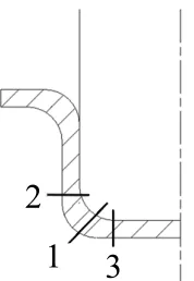
In this case the process suffers from a problem. During or after the production of the bearing tubes cracks appear. The location of the cracks are indicated by the black lines in Figure 1.2. The production process has been modified by adding an annealing step, which reduces the scrap rate, and by adding a 100% crack control to preclude that a bearing tube with a crack leaves the factory.
INPRO already investigated the problem of the bearing tube. The process was simulated with FEM software and on the basis of this simulation several adjustments were tested. The outcome of this investigation led to modifying the process by adding an extra deep drawing step with a blank holder force. More information on this investigation can be found in Appendix A. The modification resulted in a better process and significantly reduced the scrap rate. But still, some cracks occurred. In the project described in this report optimisation techniques are applied to prevent the cracks from occurring. These techniques are as well applied to the original process as to the modified process. In the remaining of the report we will refer to the original process as the
reference process.
For the optimisation the deep drawing process is simulated in the FEM simulation software Auto-Form. To the simulation results of the deep drawing process the optimisation strategy developed at the UT is applied. There are two possibilities for optimisation:
1. Optimise the reference process to compare these results with the modified process
1.3 Outline report 5
Figure 1.2: The locations where the cracks occur
2. Optimise the modified process to further reduce the scrap rate
Both optimisations are performed during this project. It shows whether the at the UT developed strategy is good applicable for an industrial case as the bearing tube and whether it is successful. The knowledge which is gained during this project can be used for further improvement of the optimisation strategy for metal forming processes using FEM.
1.3 Outline report
Chapter 2
Problem analysis: failure in deep drawing
In order to effectively remove the cracks in the bearing tube by optimisation techniques, it is es-sential to clearly understand the problem and the quantities (e.g. strains, residual stresses) that cause these cracks. If the wrong quantity is optimised, applying optimisation techniques is use-less since it will never solve the occurrence of the cracks. The cause of the cracks is therefore thor-oughly investigated in this chapter. Besides identifying which quantity needs to be optimised, it is important to know which boundaries limit the process. After all, the optimal process needs to be a feasible one. Also, for optimisation we need to know which parameters influence the process: which parameters influence the quantities that cause the cracks and which parameters influence the process boundaries. All these matters are treated in this chapter.
In Section 2.1 the deep drawing process of a simple cylindrical cup is treated to get a feeling of deep drawing processes in general. In this section possible failure mechanisms which limit this process are also described. This gives insight into the process boundaries and the parameters that are involved. The process of the bearing tube is the subject of Sections 2.2 and 2.3. In the first of these two sections, a complete picture of the situation is made and the simulation of the process is discussed. In the next section on the bearing tube, possible causes for the cracks are discussed. Finally, Section 2.4 contains some conclusions.
2.1 A cylindrical cup
This section handles the deep drawing process of a simple cylindrical cup. First, the process is treated in Section 2.1.1, including the forces which influence this process. In Section 2.1.2 dif-ferent failure mechanisms which limit the deep drawing process of a simple cylindrical cup are discussed.
2.1.1 The deep drawing process
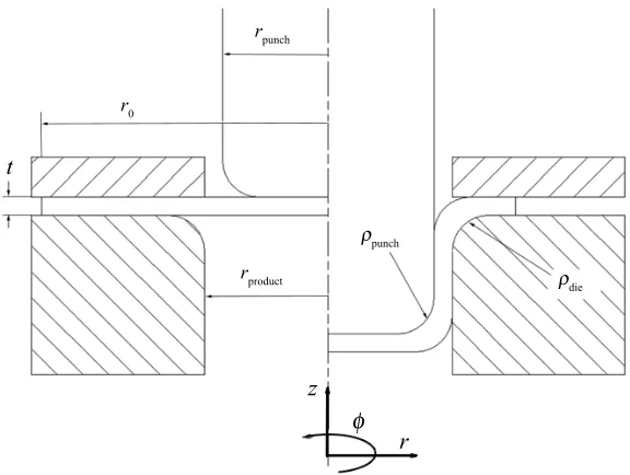
In Figure 2.1 the deep drawing process of a simple cylindrical cup is shown. It is a forming process under combined compression and tension. A flat plate is forced trough a die by a punch to form a closed-contoured, thin-walled product (circular, rectangular, oval, etc.). The material from the
flange which is drawn inside forms the wall and is stretched in axial direction (εz > 0), while
the material in the flange is stretched in radial direction, but compressed in tangential direction
(εr >0, εφ <0). An example of a deep drawn product is a sink or an aluminium beverage can.
Also, a lot of automotive parts, like body panels, are formed by the process of deep drawing.
Figure 2.1: The deep drawing process of a cylindrical cup
The process of deep drawing includes radial drawing between the die and the blank holder (the deformation of the flange), bending and unbending under tension over the rounding of the die and the rounding of the punch, stretching of the blank between the die and the punch and stretch-ing over the punch nose.
The total needed deep drawing force can be split up in the different partial forces needed to
accomplish these parts of the process. These forces are the force needed to deform the flangeF1,
the force to bend the blankF2 and the forces to overcome the friction between the flange and
the tools F3 and between the blank and the rounding of die F4. From the derivation of these
(dimensionless) forces in [24], it follows that:
F1 max = F(n, β, ε0)≈(0,75 + 0,15√n−0,35n2)(β−1)·
³n
e
´n
eε0 (2.1)
F2 = F(ε0, ρdie, t)≈
1 2ρdie
t + 1
·³ne´neε0 (2.2)
F3 = F(µflange, r0, t, n, ε0)≈0,012µflange
r0
t
³n
e
´n
eε0 (2.3)
F4 = F(µdie rounding, µflange, r0, t, n, β, ε0)≈1,6µdie rounding(F1+
1
2F2+F3) (2.4)
All parameters in these equations are summarised in Table 2.1. The total deep drawing force exists from these partial forces and thus depends on all these parameters. For the derivation of these forces, the strain hardening function defined by Equation 2.5 has been applied.
σf = (ε−ε0)n (2.5)
In this equationσfdenotes the deformation resistance,Ca characteristic value depending on the
material andεthe true strain.
2.1.2 Failure mechanisms
2.1 A cylindrical cup 9
Material parameters
n strain-hardening coefficient
ε0 prestrain
Process parameters
µflange coefficient of friction along the flange
µdie rounding coefficient of friction near the rounding of the die
Design parameters
β deep drawing ratio r0
rproduct
r0 original radius of the blank
t original thickness of the blank
ρdie rounding of the die
Table 2.1: Parameters of the deep drawing process of a simple cup
the process, because the product will fail if the total force exceeds the maximum allowable force. Failing due to too large a force is a common failure mechanism. However, there are other situa-tions in which the product does not satisfy the designed shape. In this section we will take a look into these different failure mechanisms. The most common failure mechanisms which determine the constraints of a deep drawing process are:
• fracture;
• necking;
• primary and secondary wrinkling;
• earing.
Fracture
The most important process boundary which limits the critical deep drawing force is fracture. Fracture occurs when the maximum allowable tensile stress is exceeded. The fractures mostly occur in the wall or in the bending region of the product, because the wall and the bending region have to transmit the punch load to the flange and this causes a large tensile stress. In the literature three different types of fractures during the deep drawing process of a cylindrical cup are distinguished [24]:
1. The most common fracture which acts in the transition zone between wall and bottom in the bending region near the punch radius
2. The fracture just above the bending region in the wall
3. The premature fracture which acts in the bottom at the start of the deep drawing process
occurs in the bending region, this means that the curvatures of the punch have influence on the tensile stress. The critical force then becomes:
Fcr=F(R, n, ε0, t, ρpunch, rpunch) =
µ R+ 1
√
2R+ 1
¶n+1
nn
½ t
ρpunch +
t
rpunch +e
³
n−√2R+1
R+1 ε0
´¾−1
(2.7)
whereρpunchis the rounding of the punch andrpunchthe radius. The premature fracture is caused
by badly chosen process conditions, for example the deep drawing ratioβor the rounding of the
punchρpunch. Hence, the first two types of fracture are the most common ones. The size of the
total deep drawing force depends on the parameters mentioned in Section 2.1.1. With a look at
these partial forces it can be concluded that for a chosen material (with a givenn, ε0andR) the
friction coefficients may not exceed certain limits and also the ratios ρt
die,
r0
t andβ may not be
too large. Besides that, the critical force tells us that the ratios ρpunch
t and rpunch
t are limiting the
process.
Necking
An engineering stress-strain curve for the most common steels looks like Figure 2.3 [15]. Until the
stressσethe material behaves elastically. After this point the material starts to deform plastically
and gets a higher yield strength due to hardening. However, the cross section decreases. At first the decrease of the cross section is compensated by the higher yield strength, but at a certain point the yield strength cannot compensate for it anymore. Now, the cross section reduces heavily until the material fails. This phenomenon is called necking. Also in deep drawing processes necking can be the cause of product failure: it causes the wall of the deep drawn product to thin and after excessive thinning the cup will finally break. However, this necking is localised necking.
The difference between diffuse and localised necking is shown in Figure 2.4. Diffuse necking precedes localised necking. After the diffuse neck has started to form, it is accompanied by con-traction strains in both the width and thickness direction. With a wide specimen, the width strain cannot localise rapidly, so the whole neck develops gradually and considerable extension is still possible after onset of diffuse necking. A condition will finally be reached where a sharp localised
neck can form at an angleθto the loading axis. Typically, the widthbof the neck is of the order
of the blank thicknesst, so very little additional elongation is possible before failure [14].
2.1 A cylindrical cup 11
Figure 2.4: Diffuse necking (a) and localised necking (b) [23]
Necking is mainly influenced by the n-value of the material, by the prestrain ε0 and by the
anisotropy factorR. For material with higherR-values necking occurs less rapidly and thus high
R-values positively affect the height of the deep drawn product.
It is not easy to express necking with a formula including these variables. To overcome this, Keeler and Goodwin introduced the Forming Limit Diagram (FLD). An example of an FLD is given in Figure 2.5. The Forming Limit Curve (FLC) which is shown in this figure indicates the limiting strains that sheet metal can sustain over a wide range of major to minor strain ratios. Usually the FLC is measured experimentally because, as mentioned, the theory for FLDs is not that straightforward. Once the FLC is determined the curve is supposed to stay the same. How-ever, because the limit curve is dependent on several factors you should be careful assuming this.
In case of low carbon steel, it can be shown that then- andR-values are not subject to a significant
change during deformation and indeed can be assumed constant. However, when a product is
deep drawn in different steps, the prestrainε0 differs in these steps. The influence of different
values of the prestrain on the shape of the FLC of aluminium alloy 2008-T6 is shown in Figure
2.6. In Figure 2.6a the prestrains were in uniaxial tension (forε2<0the prestrains were along the
1-direction and forε2 >0the prestrains were along the2-direction). In each case the minimum
corresponded to plane strain (ε2 = 0) during testing. In the Figure 2.6b the prestrains were in
biaxial tension.
It can also happen that there are some deviations between an experimental FLC and a theoretical
approach of the FLC. These deviations can be caused by the strain rate exponent mwhich is
Figure 2.6: Influence of prestrains in (a) uniaxial tension and (b) biaxial tension on the FLC of 2008-T6 aluminium [14]
not taken into account. The strain rate exponent can be defined asm = δlnσ
δln ˙ε and is in his turn
dependent on the temperature. Thism-value has influence on the minimum of the FLC. A change
inmcan cause critical strains to be up to 30% larger. Another deviation can be that the minimum
of the FLC is not situated atε2 = 0like theory tells us, but at slightly positive values ofε2. This
happens when the strains are measured at the outside surface of the blank while the plane strain situation is at the mid-plane of the blank.
Primary wrinkling
The compressive stress in tangential direction of the flange can be a cause of wrinkling. The remedy for this is to apply a blank holder. However, if the blank holder force is too large, the friction between the blank and the blank holder will become so large that the force to overcome this friction makes the total deep drawing force to exceed the maximum allowable force and fracture will occur. In Figure 2.7 it is shown how wrinkling depends on the blank holder force
F and the deep drawing ratioβ. For thinner blanks, the first critical line moves upwards (so
wrinkling still occurs for a larger hold-down force than thicker blanks) while the second critical line moves downwards (so fracture occurs for a smaller hold-down force than for thicker blanks), narrowing the range where a good draw occurs. Wrinkling can also be indicated with help of an
2.2 The bearing tube: the process 13
FLD, this is shown in Figure 2.5.
Besides the thicknesst, experiments have shown that higher values of the Young’s modulusE
and the strain-hardening exponentnreduce the tendency of wrinkling. Also, it is shown that the
R-value has influence on this type of wrinkling; higherR-values reduce the problem of wrinkling
[23].
Another measure which is used to prevent wrinkling, is applying draw beads. Draw beads limit the amount of material drawn into the die, which has a beneficial effect on preventing compres-sive instabilities.
Secondary wrinkling
Another form of compressive instability is called secondary wrinkling. When the rounding of
the die ρdie is too large compared to the thickness of the blank t, a large part of the blank is
not supported by the die which causes secondary wrinkling. In the same way, the ratio between
the rounding of the punch and the thickness ρpunch
t may not be too large, to prevent secondary
wrinkling near the rounding of the punch.
Earing
Anisotropy causes uneven flow, resulting in an uneven rim at the open end of the cup. When an even number of valleys and peaks are evident on the rim of the cup, the defect is called earing. A measure for the differences in the planar anisotropy, and therefore a measure for earing, is:
∆(R) =1
2(R0−2R45+R90) (2.8)
When∆(R)differs more from 0, the earing will be stronger. More earing means that the blank
needs to be larger, which results in a largerβand the process becomes more critical [1].
2.2 The bearing tube: the process
In this section the deep drawing process of the bearing tube is treated. In Section 2.2.1 the process of the bearing tube is discussed and in Section 2.2.2 the simulation of the process is treated.
2.2.1 The process
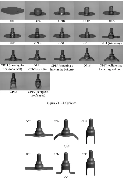
The bearing tube is being deep drawn in ten different steps. The process is shown in Figure 2.8. In OP02 to OP10 the bolt is formed. Next, the flange is trimmed and thereafter the flanges are further formed in two more deep drawing steps, OP16 and OP18. The blank is made of 3 mm thick steel; for deep drawing processes this is rather thick. The steel is a hot-rolled low carbon steel which has good deep drawing abilities. The European norm EN 10111 indicates the different qualities of hot-rolled steel for cold forming with the numbers DD10 through DD14 [3]. The higher the number, the better the formability of the steel. The steel used for this automotive part satisfies the norm for DD13. The material properties of the steel used for the bearing tube can be found in Appendix B.
The production of the parts takes place in the factory of Fischer & Kaufmann (FIuKA) which is the supplier of the product. After the production the parts are transported to a Volkswagen (VW) plant.
After the cracks had been signalised, FIuKA added an annealing step. During this annealing step,
which takes place directly after the production, the parts are kept at a temperature of200◦C for
Figure 2.8: The process
2.2 The bearing tube: the process 15
deep drawing step with a blank holder force before the last deep drawing step OP18. In this step the first part of the flanges are deformed while a blank holder forces keeps the second part of the flanges in place. The original process, referred to as the reference process, and the modified process are shown in Figure 2.9.
These two adjustments reduced the scrap rate significantly, but did not prevent all cracks from occurring [29]. Now, VW is applying a 100% crack control to prevent a part with a crack from leaving the plant. This control takes place two days after the production of the parts in the FIuKA factory when the parts arrive at the VW plant.
2.2.2 Finite Element simulation of the process
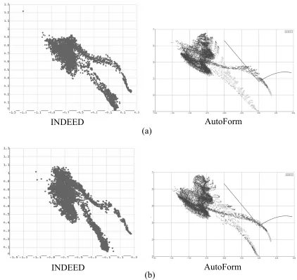
The optimisation of complex forming processes like the bearing tube is becoming possible through the use of Finite Element (FEM) simulations. Therefore, simulating the process is an important part of the optimisation procedure. INPRO already simulated the process in the simulation pro-gramme INDEED, but since INDEED is not available at the University of Twente, AutoForm is chosen to be the FEM simulation software which is being used for optimising the process of the bearing tube. Both the reference process and the modified process were modelled in AutoForm and the results were validated by comparing them to the results of INDEED and to reality.
Comparison between the AutoForm and INDEED simulations
The process was already simulated in the computer programme INDEED by INPRO. Some re-sults of the simulation in INDEED can be found in Appendix A. To be able to compare the sim-ulation in INDEED with the simsim-ulation in AutoForm the used material models were made in
Figure 2.11: The forming limit diagrams after OP18 (a) in case of the reference process and (b) in case of the modified process
accordance with each other. In Figure 2.10 the stress-strain curves and the yield loci which are used for the simulation in AutoForm and for the simulation in INDEED can be seen. Besides the used material models, differences between the outcome of both simulations can be due to for example the use of different elements or different contact algorithms. Moreover, the blank used in the INDEED simulation has a slightly different shape than the blank used in the AutoForm simulation.
2.2 The bearing tube: the process 17
Figure 2.12: Change in thickness in % (a) in case of the reference process and (b) in case of the modified process
Comparison between AutoForm and reality
The thickness over the length of the bearing tube was measured with a part of a cross-section of the bearing tube that has been produced by the modified process. This thickness is compared to the thickness resulting from the AutoForm simulation of the modified process. The measured values of the thickness can be found in Figure 2.13c and the values of the thickness as simu-lated by AutoForm in Figure 2.13b. It appears that the AutoForm simulation underestimates the thickness in the top of the tube and overestimates the thickness near the edge.
Because we are most interested in thickness over the edge where the cracks occur (the edge is indicated in Figure 2.13a), this thickness was measured for more bearing tubes. Eleven bearing tubes which are made with the modified process and two which are made with the reference process are used for this measurement. The average thickness over the edge of these tubes for both the reference and the modified process are presented in Figure 2.14. The thickness over the edge that AutoForm simulates is also presented in this figure for both processes. It is clear that magnitude of the thickness over the edge between AutoForm and reality is rather different. However, the trend in the thickness is more or less comparable and for the modified process the thickness reduced in both cases.
For optimisation, the AutoForm simulations are used as a reference situation and the differences that exist between AutoForm and INDEED and between AutoForm and reality are no further
Figure 2.14: The thickness over the edge of the bearing tube, from the left till the right corner
discussed for this project.
2.3 The bearing tube: possible causes of failure
As could be read in Section 2.2.1, some modifications to the process have been implemented after the cracks were discovered. Although this reduced the scrap rate, it did not prevent all the cracks from occurring. There have been some tests, but it was not exactly clear yet what the problem is. To gather information that could reveal the cause of the cracks several initiatives have been undertaken. These initiatives and the resulting sources of information are indicated below.
• The meeting with Mr Maschke (VW) and INPRO in Berlin
– Presentation Mr Maschke [18]
– Presentation Mr Nitsche [22]
– Material data DD13 (Norm EN 10111 - DD13) [3]
– Metallographic photos
– Bearing tubes with cracks and A-arm
• E-mail contact with Mr Maschke [17]
– Metallographic photos
– Report Volkswagen Qualit¨atssicherung [25]
• Communication with metallurgists
– Conversation with metallurgists [4]
– E-mail contact with a metallurgist [2]
– Scientific publication on Cold Work Embrittlement [20]
• A visit to the manufacturer of the bearing tubes (FIuKA, M. Schr ¨oder and J. M ¨uller) in
Finnentrop [29]
– Report Access [19]
– Metallographic photos
– Material data Hoesch (see Appendix B and [13])
– Raw material
These contacts led to two possible causes for the cracks in the bearing tube.
1. Brittle fracture or Cold Work Embrittlement 2. Large deformations due to forming
2.3 The bearing tube: possible causes of failure 19
Figure 2.15: A transgranular fracture surface (a) and an intergranular fracture surface (b) [12]
2.3.1 Brittle fracture in deep drawing processes
The most common failure mechanisms in deep drawing processes have been discussed in Section 2.1.2. These failure mechanisms do not include brittle fracture. Brittle fracture does normally not occur in deep drawing processes, because in the process the material is subject to plastic deformation and therefore it needs to be ductile. However, with the development of stronger steels which are well deformable brittle fracture is an increasing problem. In this section brittle fracture within ductile materials will be treated.
A brittle fracture occurs by rapid crack propagation and without appreciable macroscopic defor-mation [12]. There are two types of brittle fracture that differ in relation to the strain rate and the temperature. In case of the first type, a change in temperature and in strain rate causes a ductile to brittle transition. The fracture is characterised by the propagation of a brittle crack along
cer-tain crystallographic planes and istransgranular(ortranscrystalline) because the fracture passes
through the grains. The other type is anintergranularfracture (crack propagation is along grain
boundaries). This type of fracture normally results subsequent to processes that weaken or em-brittle grain boundary regions [27]. Examples of a fracture surface for both these types of fracture are shown in Figure 2.15.
As mentioned before, deep drawing processes become more susceptible to brittle fracture. This is because more low carbon interstitial free (IF) steels are used. These steels have excellent deep
drawing abilities which result from extra low carbon and nitrogen contents (<50 ppm) in
addi-tion to titanium and niobium microalloying for stabilising interstitial elements such as carbon. Thus these strong, good deformable steels seem very suitable for deep drawing processes and
therefore it is more and more used. However, IF steels are susceptible toCold Work
Embrittle-ment(CWE). CWE is a phenomenon which occurs in secondary forming operations and causes a
Figure 2.16: A fracture limit in an FLD
The propagation of the crack is dependent on the temperature and the applied stress (residual stresses in the material and externally applied stresses). Besides that, grain boundary weaken-ing elements, such as phosphorus, increase the susceptibility to CWE, where grain boundary strengthening elements, such as boron and free carbon, decrease the susceptibility. Another in-teresting note is that there seems to exist a relation between the equivalent plastic strain and the ductile to brittle transition temperature which is of importance in case of CWE [20].
2.3.2 Large deformations
Large deformations due to forming can cause fracture. The ten step deep drawing process of the
bearing tube causes the prestrainε0 to differ. In Section 2.1.2 it was mentioned that this
influ-ences the position of the Forming Limit Curve (FLC). Figure 2.6a showed that prestraining in
1-direction, which is the case in the flange during deep drawing processes, causes the FLC to
raise for larger minor strains and the necking limit will be exceeded at higher strains. For small minor strains the FLC barely changes. The variation in prestrain is thus not expected to be the cause of the cracks in the critical areas which are dealing with small minor cracks after the last deep drawing step.
However, besides the necking limit it is also possible to show a fracture limit in a Forming Limit Diagram (FLD). An example of a fracture limit curve in an FLD is shown in Figure 2.16. Usually local necking occurs before fracture, but with an unfavorable combination of load and material structure, fracture can occur before necking becomes a problem.
2.3.3 Discussion
In case of the bearing tube there are reasons to believe that the brittle fracture as described in Section 2.3.1 is causing the cracks. Brittle fracture as cause for the cracks in the bearing tube is supported by the following observations:
• Delayed cracking is reported for the bearing tubes [18, 29];
• Metallographic photos present intergranular cracks (see Figure 2.18);
• The DD13 material norm indicates a quite high percentage of phosphorus (0.030%) [3],
which weakens the grain boundaries;
• An annealing heat treatment to reduce the residual stresses has significantly reduced the
scrap rate [29, 17].
2.4 Conclusions 21
Figure 2.17: The equivalent strain in (a) the reference process and (b) the modified process.
plastic strain. This supports the conclusion that the cause of the cracks is not influenced by the equivalent plastic strain which seems to be related to CWE [20].
On the other hand, an investigation of VW tells us that the cause of the cracks should be sought in a critical forming step when the flange is drawn in the direction of the bolt (OP18). During this forming step the strains at the critical areas increase considerably. Due to work hardening at this location, the material loses its ductility which can finally lead to cracks [25]. Metallurgist confirm that this can be a possible cause [4]. This cause is supported by the following observations:
• Finite Element simulations performed by INPRO have shown large strains in the critical
areas (see Figure 2.11. Reducing these strains by adding another forming step before Oper-ation 18 has significantly reduced the scrap rate [29, 22];
• An annealing heat treatment to reduce the effect of work hardening in the critical areas has
also reduced the scrap rate [29, 17].
The above observations lead us to believe that the large deformations due to forming is the cause to focus on for optimisation. The cracks are not (always) there directly after the deep drawing process (in that case, annealing would not help), but the large amount of deformation and work hardening is responsible for the delayed crack occurrence. Therefore, we will - just as was done by INPRO - focus on reducing the major- and minor-strains, rather than the equivalent plastic strain and residual stresses that would have been more interesting in case brittle fracture were the cause.
2.4 Conclusions
This chapter provided background on deep drawing processes by treating the deep drawing process of a simple cylindrical cup. Also, the most common failure mechanisms for deep drawing processes are treated:
• fracture;
• necking;
• primary and secondary wrinkling;
Figure 2.18: Intergranular crack
This gave insight into the different parameters that influence the deep drawing process. Table 2.2
gives an overview of the variables that influence the deep drawing process. In this tableFis the
deep drawing force andFcrthe critical force related to fracture.rpunch,r0,ρpunchandρdiedenote
respectively the radius of the punch and the original radius of the blank and the rounding of the punch and the die.
This chapter also introduced the process of the bearing tube. Both the reference and the modified process as proposed by INPRO are mentioned. FEM simulations of both processes have been made in AutoForm. These simulations are compared to reality and to the simulations made by INPRO in the FEM programme INDEED. The differences are discussed, however the AutoForm simulations are used as a reference situation for the optimisations that are performed in Chapters 4 and 5.
After having gathered further information on the process, two possible causes for the cracks were identified:
1. Brittle fracture or Cold Work Embrittlement (CWE) 2. Large deformation due to forming
parameter influence parameter on the deep drawing forceF and on the different failure mechanisms
Material parameters
n strain-hardening coefficient F, Fcr, necking, primary wrinkling
ε0 prestrain F, Fcr, necking
R anisotropy factor Fcr, necking, primary wrinkling, earing
E Young’s modulus primary wrinkling
Process parameters
µ friction coefficient F
Design parameters
β deep drawing ratio F
t thickness primary wrinkling
rpunch
t Fcr
r0
t F
ρpunch
t Fcr, secondary wrinkling
ρdie
t F, secondary wrinkling
2.4 Conclusions 23
Chapter 3
Optimisation theory
For this project the optimisation strategy for metal forming processes which is being developed at the University of Twente (UT) is applied. In this chapter the theory behind this strategy is treated. Section 3.1 starts with a short overview of the optimisation strategy. The other sections treat the theory behind the different steps in this optimisation strategy as can be seen in Figure 3.3. Section 3.9 finalises this chapter with some conclusions.
3.1 The optimisation strategy developed at the University of Twente
The optimisation strategy couples a mathematical optimisation procedure to Finite Element Method (FEM) calculations. Making the optimisation problem suitable for optimisation is an important part of the procedure, this is done by modelling. The interaction between modelling the problem and solving it is shown in Figure 3.1.
The modelling should be done cleverly to prevent that the optimisation problem that was mod-elled can finally be solved efficiently by a suitably chosen optimisation algorithm. Modelling should result in a set of variables to describe the design alternatives, an objective function and a set of constraints. How these quantities relate to FEM is displayed in Figure 3.2. Some quantities are known beforehand, where others are not. Design variables and explicit constraints which ex-plicitly depend on these design variables are known beforehand and are the input for FEM. The output of the FEM simulation delivers quantities which implicitly depend on the design vari-ables. The objective function is generally such an implicit quantity and it is also possible to have implicit constraints.
After the problem is modelled it can be solved by applying a suitable optimisation algorithm. For the strategy a metamodel based sequential approximate optimisation algorithm is chosen. This algorithm is extensively described by Bonte in [11]. Background on choices made for this algorithm is provided in [6, 8, 9, 16]. The steps the algorithm comprises are shown in Figure
3.3. It starts with a Design Of Experiments for cleverly choosing experimental points for which responses should be calculated by running FEM simulations. Next, a metamodel is fitted through these responses. This metamodel approximates the true response function. Optimising this model by applying an algorithm will give the solution of the optimisation problem. Because this is an approximation it needs to be validated by running a FEM calculation with the optimal settings. When the solution is not accurate enough more experimental points need to be added and the process starts over again until an optimum is found which is accurate enough. This process is called sequential improvement. Finally, the result of the optimisation procedure provides the optimal values for the design variables.
As shown in Figure 3.1 there exists interaction between the modelling and the solving of the optimisation problem. It means that the optimisation algorithm should be compatible with the model of the optimisation problem in order to solve the optimisation problem both effectively and efficiently. With this in mind it should be noted that the optimisation algorithm which is
used for the strategy suffers from thecurse of dimensionality, which means that it becomes
ex-ponentially more time consuming to solve when more design variables are taken into account. Therefore the number of variables will be limited as much as possible. This is done by screening the variables. In the screening process the influence of every variable on the objective function is evaluated (taking into account the set of constraints), making it possible to choose an appropriate set of variables for the optimisation.
The different steps of the optimisation strategy are treated in the next sections as displayed in Figure 3.3.
3.2 Modelling 27
3.2 Modelling
The first step of any mathematical optimisation procedure is modelling the problem. This is an important step which always should be done carefully, because if the problem is not properly modelled, the optimisation will not give a useful result. A mathematical optimisation model consists of:
• design variables;
• an objective function;
• constraints.
Bonte proposes a structured procedure to model optimisation problems in metal forming pro-cesses [10]. With this procedure the variables, the objective function and the constraints are iden-tified by following different steps. This procedure is applied to the optimisation strategy. In this section this procedure as elaborated in [10] is summarised.
The procedure is based on the Product Development Cycle, which is a part of the Product Life Cycle. The Product Development Cycle is equal to the Product Life Cycle minus the stages 6 and 7 as presented in Figure 3.4. The Product Development Cycle is applicable to any kind of product. When applied to metal formed products, there are five groups of quantities which can be identified to be influencing the Production Development Cycle (these are indicated in Figure 3.4):
• Functional Requirements: these are product properties that are critical to customer
satisfac-tion and product funcsatisfac-tionality;
• Design Parameters: these define the product design;
• Process Variables: these are process settings necessary to manufacture the product;
• Defects;
• Costs.
Relevant metal forming quantities can be subdivided into these groups. With help of top-down structures which are made for each group all metal forming related quantities can be defined. Examples of these top-down structures can be found in [[10]]. For modelling optimisation prob-lems in metal forming a seven step procedure based on this Product Development Cycle can be
the constraints. It includes the following steps:
1. Determine the appropriate optimisation situation 2. Select only the necessary responses
3. Select one response as objective function, the others as implicit constraints 4. Quantify the objective function and implicit constraints
5. Select possible design variables
6. Define the ranges on the design variables 7. Identify explicit constraints
Step 1: Determine the appropriate optimisation situation
For modelling optimisation problems in metal forming processes, we focus on the stages 2 through 5 of of the Product Life Cycle. Within this part of the Product Design Cycle, four situations in which the optimisation of metal products and their manufacturing processes can play a role are distinguished:
• Part Design, where it is aimed to optimise the metal formed product’s Functional
Require-ments by determining the Design Parameters.
• Process Design Type I, where it is aimed to exactly obtain the Design Parameters set by
the part designer by determining the Process Variables. Alternatively, one can aim to man-ufacture a defect free product or minimise production costs by determining the Process Variables.
• Process Design Type II, where it is aimed to optimise the metal formed product’s Functional
Requirements by determining the Process Variables. Design Parameters, Defects and Costs can still play a role in parallel to the Functional Requirements.
• Production, where optimisation techniques can be used to solve manufacturing problems.
These situations and their relations to the Product Development Cycle are also presented in Fig-ure 3.4. To demonstrate how optimisation can be applied to one of these four situations, compare the input-response model for optimisation in Figure 3.2 to that for a Process Design Type I prob-lem in Figure 3.5. Note the resemblance: one can immediately observe that for a Process Design Type I problem, the objective function and implicit constraints are the Design Parameters, Defects and Costs, whereas the design variables are related to the Process Variables.
Steps 2 to 4: Define responses
In steps 2 to 4 the responses are defined. In step 2, top-down structures can be used to select the necessary responses for the specific problem. Subsequently, in step 3, one of the defined response quantities is selected as objective function, the others as implicit constraints. Next, the responses need to be quantified. This is done in step 4.
3.3 Screening 29
Type of response No nodal/element Nodal/element Nodal/element
value value, critical value, non-critical
Objective function, no target minX min maxNX min
P
N(X)
N
Objective function, target =X0 min|X−X0| min maxN|X−X0| min||X−√XN0||2
Implicit constraint, USL X−U SL≤0 maxN(X−U SL)≤0
Implicit constraint, LSL LSL−X ≤0 maxN(LSL−X)≤0
Table 3.1: Response quantification [10]
further into critical and non-critical values. Critical values are the values for which none of the nodal/element values is allowed to exceed a specified level. If it is acceptable that some of the nodal/element values exceed this specified level, but important that the average response value performs well, the response is non-critical. Constraints are by definition critical values.
For the usage of the software belonging to the applied optimisation strategy, the objective func-tion needs to be defined in such a way that it is minimised. The formulafunc-tion of a constraint should be such that it delivers a positive value when the limit is exceeded and the response does not sat-isfy the constraint.
Step 5 to 7: Define input quantities
In steps 5 to 7 the FEM inputs are defined. These are the design variables and explicit constraints which depend on these variables. Steps 5 and 6 comprise the selection and quantification of the design variables. The optimisation problem selected in step 1 determines the groups of design variables to take into account. Subsequently, top-down structures can be used to select the vari-ables. This is done in step 5. In step 6 the upper and lower bounds of all design variables are determined. Step 7 deals with the explicit constraints. Explicit constraints describe impossible combinations of the design variables.
This 7 step methodology is generally applicable to any metal forming problem and yields a spe-cific mathematical optimisation model, which can subsequently be solved using a suitable opti-misation algorithm.
3.3 Screening
Since the applied optimisation strategy suffers from thecurse of dimensionality, it is useful to
limit the number of variables taken into account for optimisation. This is done by a screening ex-periment. Such an experiment is designed to investigate variables with a view toward eliminating the unimportant ones. The influences of the different variables on the responses are investigated and these influences are evaluated by a Pareto analysis. A Pareto analysis is based on the 80-20 rule which is supported by experiences in many fields. For example, in many stores 80% of the profit is realised by 20% of the products. Likewise, it is often the case that 80% of quality prob-lems are caused by 20% of the possible causes. In this case, it will be tried to obtain the variables that determine 80% of the variations in the responses by a Pareto analysis. After the number of variables is reduced, optimisation will be more efficient and require fewer FEM runs.
Figure 3.6: The response function of a22factorial design
this section [21]. After running the FEM simulations, the effect of the variables on the responses is analysed by Pareto and effect plots.
3.3.1 Two-level full factorial designs
In case of screening for the optimisation strategy the variables vary between only two values, their minimum and their maximum value. It is tried, by setting up several computer experiments with different combinations of these input values, to determine the influence of the different variables on the optimisation problem. This is an efficient way for getting a rough estimation on the influence, because it requires only few calculations.
Such an experimental design is called2k factorial design because it defines exactly2k runs. We
will demonstrate this by giving the example of a22full factorial design which can be used in case
of two variables. This design denotes four experiments with the following combinations of the
variablesaandb:
• (amin,bmin)
• (amin,bmax)
• (amax,bmin)
• (amax,bmax)
An example of such an experimental design and its response can be seen in Figure 3.6. With
the response of these runs the main effects and interaction effect of the variablesa and b on
the response can be evaluated. The magnitude and direction of the effects can be examined to determine which variables are likely to be important. For example, in Figure 3.6 it can be seen
that the main effect of variableais significantly larger than the main effect of variableb.
3.3.2 Fractional factorial designs
With an increasing number of variables in a2k factorial design, the number of required runs
for a complete replicate of the design grows rapidly. For example, a complete replicate of the26
3.3 Screening 31
interactions may be obtained by running only a fraction of the complete factorial experiment. These fractional factorial designs are among the most widely used types of design in industry. The purpose of screening is to identify the variables that have large effects and therefore it can be satisfactory only to look at a fraction of the factorial experiment.
The successful use of fractional factorial designs is based on three key ideas [21]:
• The sparsity-of-effects principle. When there are several variables, the system or process is
likely to be driven primarily by some of the main effects and low-order interactions.
• The projection property. Fractional factorial designs can be projected into stronger (larger)
designs in the subset of significant variables.
• Sequential experimentation. It is possible to combine the runs of two (or more) fractional
factorials to assemble sequentially a larger design to estimate the factor effects and interac-tions of interest.
On account of the sparsity-of-effects principle, in many cases we learn enough from the fractional design to proceed to the next stage of experimentation, which might involve adding or removing variables, changing responses, or varying some of the variables over new ranges. And if we have not learned enough, we can apply sequential experimentation and expand the experiment.
3.3.3 The resolution of a design
A2k fractional design containing2k−p runs is called a1/2p
fraction of the 2k design or, more
simply, a 2k−p fractional factorial design. An example of a fractional factorial design is a23−1
resolutionIIIdesign (see Figure 3.7). A resolutionIIIdesign means that main effects are aliased
with two-factor interactions. A design is of resolutionRif nop-factor effect is aliased with another
effect containing less thanR−pfactors. Designs of resolutionIII,IVandVare used for screening
for the optimisation strategy treated in this chapter. The definitions of these designs follow below [21].
• ResolutionIIIdesigns. These are designs in which no main effects are aliased with any other
effect, but main effects are aliased with two-factor interactions and two-factor interactions may be aliased with each other.
• ResolutionIVdesigns. These are designs in which no main effect is aliased with any other
main effect or with any two-factor interaction, but two-factor interactions are aliased with each other.
• ResolutionVdesigns. In these designs main effects are not aliased with each other nor with
two-factor interactions, two-factor interactions are not aliased with each other either, but they are aliased with three-factor interactions.
x2 x3 x1
0 0%
(a)
−1 −0.5 0 0.5 1 3500 4000 4500 5000 5500 6000 6500 x1 f1
−1 −0.5 0 0.5 1 3500 4000 4500 5000 5500 6000 6500 x2 f1
−1 −0.5 0 0.5 1 3500 4000 4500 5000 5500 6000 6500 x3 f1 (b)
Figure 3.8: Analysis of the effect of the variables on the response by (a) a Pareto plot and (b) effect plots
We usually like to employ fractional designs that have the highest possible resolution consis-tent with the degree of fractionation required. The higher the resolution, the less restrictive the assumptions that are required regarding which interactions are negligible in order to obtain a unique interpretation of the data. However, for a higher resolution design more calculations are required. The choice thus depends on the desired accuracy considering the calculation time.
3.3.4 Analysis with Pareto and effect plots
The responses of the the design points are analysed by applying an ANalysis Of VAriance (ANOVA), see Myers and Montgomery [21]. This statistical technique is used to determine the effects of the different variables on the responses. The figures following from the ANOVA are used for Pareto and effect plots. Examples of a Pareto and effect plots are presented in Figure 3.8. The propor-tional effects on the responses are displayed by the Pareto plot and the amount and direction of the effect of each variable on the response is displayed in the effect plots. In the example of Figure
3.8 the variablex2determines almost 80% of the effect on the response and could thus be chosen
to be kept in the optimisation model whereas the variablesx1andx3may be omitted.
3.4 Design Of Experiments
3.4 Design Of Experiments 33
Figure 3.9: The bias error of a linear metamodel which approximates a quadratic response func-tion constructed from (a) DOE points on the boundary of the design space and (b) from DOE points in the interior of the design space [11]
functions. The metamodels used in this optimisation strategy are based on two methods, referred to as Design and Analysis of Computer Experiments (DACE) and Response Surface Methodol-ogy (RSM). The metamodels based on DACE and RSM are further discussed in Section 3.5. In this section it is also concluded that DACE seems to be slightly more suitable for optimisation problems of metal forming processes than RSM. Therefore the applied DOE strategy is primary adjusted to a DACE based metamodel.
3.4.1 Properties of the DOE strategy
For DACE a good experimental design should:
• result in a good fit of the response;
• be cost-effective.
For a good fit of the response the design points should cleverly be chosen taking into account the shape of the metamodel. In the case of DACE the functions determining the metamodel are extremely flexible. Therefore, no assumption can be made for the final shape of the metamodel and it is important to gather information on the investigated phenomenon throughout the entire design space. Another interesting issue is the presence of a random error. This error is present in stochastic models. The metamodels based on RSM possess such an error (see Equation 3.1 in Section 3.5). The random error has an influence on the metamodel. However, for deterministic computer experiments no random error term is present. If an error is present, this is a bias error. A bias error is an error which evolves when the true response is of a different shape than the presumed metamodel. Generally, the bias error increases when DOE points are located on the boundaries of the design space. This is demonstrated in Figure 3.9. Noticing these facts gives reason to choose a DOE strategy for which the experimental design points are evenly spread over the (interior of the) entire design space [11]. Such a design is called a spacefilling design. Besides points in the interior of the design space, points on the boundary are also of interest in case of optimisation. For optimisation it is important that the metamodel gives accurate results in the neighbourhood of the optimum. Often, this optimum will be constrained and thus will be located at the boundary of the design space. Therefore, an accurate prediction is needed on the boundary, which implies performing measurements on the boundary.
misations strategy and is treated in Section 3.8.
Concluding, the DOE strategy should satisfy the following properties:
• be spacefilling;
• have design points on the boundaries of the design space;
• eliminate replicate points.
3.4.2 The DOE strategy
Bonte conducted a study to different DOE strategies and concluded that a Latin Hybercube De-sign (LHD) is a suitable strategy for the applied optimisation algorithm for metal forming pro-cesses [11]. Such a design excludes duplicate points and is easily made spacefilling.
Applying LHD comprises dividing the design space into a number of cubes and choosing one measurement randomly in one cube. In Figure 3.10a this is presented for a two-dimensional case; each column or row of the design comprises only one measurement. Since spacefillingness is
es-sential the LHD is modified with themaximin criterion, which maximises the minimum distance
between the design points. The maximin criterion ensures that no two design points are too close to each other. The combination results in a spacefilling Latin Hypercubes Design as shown in Figure 3.10b, which is a very powerful DOE strategy for DACE [26]. The maximin criterion is also applied when new design points are added by the user for improving the accuracy of the metamodels.
An LHD will generally provide design points in the interior of the design space and hardly any on the boundary. To compensate for this lack of points on the boundary, the LHD is combined with a full factorial design, which places DOE points right in the corners of the design space in a 2-dimensional case (see Figure 3.10c).
An advantage of LHD is that it provides excellent projection properties. Suppose one of two design variables appear to be not significant, then all measurements in that dimension can be
3.5 Fitting the metamodel 35
skipped. Using LHD, the expensive simulations that have already been preformed by then, can be projected onto the other dimension resulting in a uniform distribution in this other dimension.
3.5 Fitting the metamodel
To approximate the response functions metamodelling is applied. A metamodel approximates the response function knowing only the response values for a number of points, namely the DOE points. Two types of metamodelling are applied: Response Surface Methodology (RSM) and Design and Analysis of Computer Experiments (DACE) [7].
3.5.1 RSM
Applying RSM, natural variables are first transformed to coded variables which are dimension-less with mean zero and with the same spread or standard deviation, i.e. the errors are assumed to be uncorrelated and to have no regularities between them. Next, regression coefficients are
obtained by least square regression. The response functionycan now be expressed by the design
matrixXcontaining the coded experimental design points, the regression coefficientsβand the
random error termεaccording to the following equation [21]:
y=Xβ+ε (3.1)
The metamodel approximates the response function with:
ˆ
y=X ˆβ (3.2)
The metamodels can have different shapes. For the optimisation algorithm four metamodels with a different shape are defined. The response is approximated by the models mentioned below. The definition of the models are given in case of two variables.
• Linear:yˆ=β0+β1x1+β2x2
• Interaction:yˆ=β0+β1x1+β2x2+β12x1x2
• Elliptic:yˆ=β0+β1x1+β2x2+β11x12+β22x22
• Quadratic:yˆ=β0+β1x1+β2x2+β11x12+β22x22+β12x1x2
The linear model is a model including only the main effects between the variables. The interaction model includes interaction between variables. These first order models are suitable for a small region where there is only little curvature in the response function. Second order models are better suitable for regions with substantial curvature in the true response functions as is the case in the neighbourhood of an optimum. An advantage of RSM is that the regression coefficients
βare determined easily by applying the method of least squares. An example of a linear RSM
based metamodel is shown in Figure 3.11 [11].
When the model is fitted, the metamodel predicted variance of any point var(ˆy∗)can be
deter-mined, and also the error varianceσ2can be estimated by the mean squared error (MSE):
MSE = SSE
n−p=
Pn
i=1(yi−yˆi)2
n−p (3.3)
where SSE is the sum of squared errors, which equals the square of the difference between the
measured response points and the response points predicted by the polynomial metamodel.nis
the total number of measurements, whereaspis the number of regression coefficients. The
Figure 3.11: Fitting a RSM and a DACE metamodel [11]
3.5.2 DACE
A variant on the Response Surface Methodology is Design and Analysis of Computer Experi-ments (DACE), also called Kriging. Using Kriging, an interpolation model is fitted through all
responses of the experimental points using a stochastic functionZ. Whereas RSM is known to
have restricted model flexibility and is primarily used for the global investigation of optima, Kriging models are known to capture local behaviour better. A Kriging metamodel is defined as:
ˆ
y=Xβ+Z(x) (3.4)
The first part of the equation covers a global trend. The Gaussian stochastic processZ which
ac-counts for the local deviation of the data from the linear regression metamodel has zero mean,
varianceσ2
z, and a covariance which includes a Gaussian exponential correlation functionR(θ,x).
The unknown parameters β, σz and θ are estimated using Maximum Likelihood Estimation,
which is generally considered to be the best way [26]. The influence of the magnitude of θ is
visualised in Figure 3.12 [11].
For the optimisation strategy three types of Kriging models are applied. For the different types different polynomials are used as a regression model:
• Kriging with a0thorder polynomial as a trend function
• Kriging with a1storder polynomial as a trend function
• Kriging with a2ndorder polynomial as a trend function
The DACE based metamodel shown in Figure 3.12 for example makes use of a0thorder
polyno-mial.
After fitting the metamodel, it can predict the response value of an unknown pointy∗(x∗)at the
location defined by the design vectorx∗. Just as for RSM, the mean squared error (MSE) can be
determined. The MSE aty∗is expressed by:
MSE (y∗) =σ2
z
µ
1−£
fT rT ¤ ·
0 FT
F R
¸ ·
f r
¸
(3.5)
This MSE equals0in casey∗equals a known measurement point. In case of applying DACE the


![Figure 2.4: Diffuse necking (a) and localised necking (b) [23]](https://thumb-us.123doks.com/thumbv2/123dok_us/1166112.1146739/19.595.219.381.599.729/figure-diffuse-necking-a-and-localised-necking-b.webp)
![Figure 2.6: Influence of prestrains in (a) uniaxial tension and (b) biaxial tension on the FLC of2008-T6 aluminium [14]](https://thumb-us.123doks.com/thumbv2/123dok_us/1166112.1146739/20.595.225.382.567.722/figure-inuence-prestrains-uniaxial-tension-biaxial-tension-aluminium.webp)