R E S E A R C H
Open Access
SSIM-inspired image restoration using sparse
representation
Abdul Rehman
1*, Mohammad Rostami
1, Zhou Wang
1, Dominique Brunet
2and Edward R Vrscay
2Abstract
Recently, sparse representation based methods have proven to be successful towards solving image restoration problems. The objective of these methods is to use sparsity prior of the underlying signal in terms of some dictionary and achieve optimal performance in terms of mean-squared error, a metric that has been widely criticized in the literature due to its poor performance as a visual quality predictor. In this work, we make one of the first attempts to employ structural similarity (SSIM) index, a more accurate perceptual image measure, by incorporating it into the framework of sparse signal representation and approximation. Specifically, the proposed optimization problem solves for coefficients with minimum L0 norm and maximum SSIM index value.
Furthermore, a gradient descent algorithm is developed to achieve SSIM-optimal compromise in combining the input and sparse dictionary reconstructed images. We demonstrate the performance of the proposed method by using image denoising and super-resolution methods as examples. Our experimental results show that the proposed SSIM-based sparse representation algorithm achieves better SSIM performance and better visual quality than the corresponding least square-based method.
1 Introduction
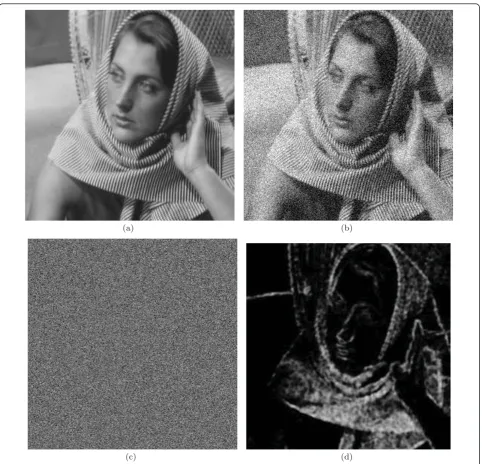
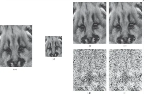
In many signal processing problems, mean squared error (MSE) has been the preferred choice as the optimization criterion due to its ease of use and popularity, irrespec-tive of the nature of signals involved in the problem. The story is not different for image restoration tasks. Algorithms are developed and optimized to generate the output image that has minimum MSE with respect to the target image [1-6]. However, MSE is not the best choice when it comes to image quality assessment (IQA) and signal approximation tasks [7]. In order to achieve better visual performance, it is desired to modify the optimization criterion to the one that can predict visual quality more accurately. SSIM has been quite suc-cessful in achieving superior IQA performance [8]. Fig-ure 1 demonstrates the difference between the performance of SSIM and absolute error (the bases for Lp, MSE, PSNR, etc.). Figure 1c shows the quality map
of the image 1b with reference to 1a, obtained by calcu-lating the absolute pixel-by-pixel error, which forms the basis of MSE calculation for quality evaluation. Figure
1d shows the corresponding SSIM quality map which is used to calculate the SSIM index of the whole image. It is quite evident from the maps that SSIM performs a better job in predicting perceived image quality. Specifi-cally, the absolute error map is uniform over space, but the texture regions in the noisy image appear to be much less noisier than the smooth regions. Clearly, the SSIM map is more consistent with such observations.
The SSIM index and its extensions have found a wide variety of applications, ranging from image/video coding i.e., H.264 video coding standard implementation [9], image classification [10], restoration and fusion [11], to watermarking, denoising and biometrics (see [7] for a complete list of references). In most existing works, however, SSIM has been used for quality evaluation and algorithm comparison purposes only. SSIM possesses a number of desirable mathematical properties, making it easier to be employed in optimization tasks than other state-of-the-art perceptual IQA measures [12]. But, much less has been done on using SSIM as an optimiza-tion criterion in the design and optimizaoptimiza-tion of image processing algorithms and systems [13-19].
Image restoration problems are of particular interest to image processing researchers, not only for their prac-tical value, but also because they provide an excellent
* Correspondence: [email protected] 1
Department of Electrical and Computer Engineering, University of Waterloo, Waterloo, ON, N2L 3G1 Canada
Full list of author information is available at the end of the article
test bed for image modeling, representation and estima-tion theories. When addressing general image restora-tion problems with the help of Bayesian approach, an image prior model is required. Traditionally, the pro-blem of determining suitable image priors has been based on a close observation of natural images. This leads to simplifying assumptions such as spatial smooth-ness, low/max-entropy or sparsity in some basis set. Recently, a new approach has been developed for learn-ing the prior based on sparse representations. A diction-ary is learned either from the corrupted image or a
high-quality set of images with the assumption that it can sparsely represent any natural image. Thus, this learned dictionary encapsulates the prior information about the set of natural images. Such methods have pro-ven to be quite successful in performing image restora-tion tasks such as image denoising [3] and image super-resolution [5,20]. More specifically, an image is divided into overlapping blocks with the help of a sliding win-dow and subsequently each block is sparsely coded with the help of dictionary. The dictionary, ideally, models the prior of natural images and is therefore free from all
(a) (b)
(c) (d)
kinds of distortions. As a result the reconstructed blocks, obtained by linear combination of the atoms of dictionary, are distortion free. Finally, the blocks are put back into their places and combined together in light of a global constraint for which a minimum MSE solution is reached. The accumulation of many blocks at each pixel location might affect the sharpness of the image. Therefore, the distorted image must be considered as well in order to reach the best compromise between sharpness and admissible distortions.
Since MSE is employed as the optimization criterion, the resulting output image might not have the best per-ceptual quality. This motivated us to replace the role of MSE with SSIM in the framework. The solution of this novel optimization problem is not trivial because SSIM is non-convex in nature. There are two key problems that have to be resolved before effective SSIM-based optimization can be performed. First, how to optimally decompose an image as a linear combination of basis functions in maximal SSIM, as opposed to minimal MSE sense. Second, how to estimate the best compro-mise between the distorted and sparse dictionary recon-structed images for maximal SSIM. In this article, we provide solutions to these problems and use image denoising and image super-resolution as applications to demonstrate the proposed framework for image restora-tion problems.
We formulate the problem in Section 2.1 and provide our solutions to issues discussed above in Sections 2.2 and 2.3. Section 3.1 describes our approach to denoise the images. The proposed method for image super-reso-lution is described in Section 3.2 and finally we con-clude in Section 4.
2 The proposed method
In this section we will incorporate SSIM as our quality measure, particularly for sparse representation. In con-trast to what we may expect, it is shown that sparse representation in minimal L2 norm sense can be easily
converted to maximal SSIM sense. We will also use a gradient descend approach to solve a global optimiza-tion problem in maximal SSIM sense. Our framework can be applied to a wide class of problems dealing with sparse representation to improve visual quality.
2.1 Image restoration from sparsity
The classic formulation of image restoration problem is as following:
y=x+n (1)
wherexÎℝn,yÎℝm,nÎ ℝm, and F Îℝmxn. Here
we assume x andy are vectorized versions, by column
stacking, of original 2-D original and distorted images,
respectively. n is the noise term, which is mostly
assumed to be zero mean, additive, and independent Gaussian. Generally m<nand thus the problem is ill-posed. To solve the problem assertion of a prior on the original image is necessary. The early approaches used least square (LS) [21] and Tikhonov regularization [22] as priors. Later minimal total variation (TV) solution [23] and sparse priors [3] were used successfully on this problem. Our focus in the current work is to improve algorithms, in terms of visual quality, that assert sparsity prior on the solution in term of a dictionary domain.
Sparsity prior has been used successfully to solve dif-ferent inverse problems in image processing [3,5,24,25]. If our desired signal, x, is sparse enough then it has been shown that the solution to (1) is the one with
maximum sparsity which is unique (within some -ball
around x) [26,27]. It can be easily found by solving a linear programming problem or by orthogonal matching pursuit (OMP). Not all natural signals are sparse but a wide range of natural signals can be represented sparsely in terms of a dictionary and this makes it possible to use sparsity prior on a wide range of inverse problems. One major problem is that the image signals are considered to be high dimensional data and thus, solving (1) directly is computationally expensive. To tackle this pro-blem we assume local sparsity on image patches. Here, it is assumed that all the image patches have sparse representation in terms of a dictionary. This dictionary can be trained over some patches [28].
Central to the process of image restoration, using local sparse and redundant representations, is the solution to the following optimization problems [3,5],
ˆ
αij= arg min
α μijα0+
α−RijX 2
2, (2)
ˆ
X= arg min
x
X−W22+λDHX−Y22. (3)
where Y is the observed distorted image, X is the
unknown output restored image, Rij is a matrix that
extracts the (ij) block from the image,Ψ Îℝnx kis the dictionary with k>n, aij is the sparse vector of coeffi-cients corresponding to the (ij) block of the image, Xˆ is the estimated image,l is the regularization parameter,
and W is the image obtained by averaging the blocks
obtained using the sparse coefficients vectors αˆij
equivalent to (4). As to the coefficients μij, those must be location dependent, so as to comply with a set of constraints of the form α−RijX
2
2≤T. Solving this
using the orthonormal matching pursuit [29] is easy, gathering one atom at a time, and stopping when the error α−RijX22 goes belowT. This way, the choice
ofμijhas been handled implicitly Equation (3) applies a global constraint on the reconstructed image and uses the local patches and the noisy image as input in order to construct the output that complies with local-sparsity and also lies within the proximity of the distorted image which is defined by amount and type of distortion.
ˆ
αij= arg min
α α0subject to
α−RijX22≤T (4)
In (3), we have assumed that the distortion operatorF
in (1) may be represented by the productDH, whereH
is a blurring filter andD the downsampling operator.
Here we have assumed each non-overlapping patch of the images can be represented sparsely in the domain of
Ψ. Assuming this prior on each patch (2) refers to the sparse coding of local image patches with bounded prior, hence building a local model from sparse repre-sentations. This enables us to restore individual patches by solving (2) for each patch. By doing so, we face the problem of blockiness at the patch boundaries when denoised non-overlapping patches are placed back in the image. To remove these artifacts from the denoised images overlapping patches are extracted from the noisy image which are combined together with the help of (3). The solution of (3) demands the proximity between the noisy image, Y, and the output image X, thus enforcing
the global reconstruction constraint. The L2 optimal
solution suggests to take the average of the overlapping patches [3], thus eliminating the problem of blockiness in the denoised image.
As stated earlier, we propose a modified restoration method which incorporates SSIM into the procedure defined by (2) and (3). It is defined as follows,
ˆ
αij= arg min
α μijα0+ (1−S(α,RijX)), (5)
ˆ
X= arg max
x
S(W,X) +λS(DHX,Y), (6)
whereS(·,·) defines the SSIM measure. The expression for SSIM index is
S(a,y) = 2μaμy+C1
μ2
a+μ2y+C1
2σa,y+C2
σ2
a +σy2+C2
, (7)
with μa andμythe means of a andyrespectively, σ2
a
and σy2 the sample variances of a and y respectively, andsaythe covariance between aandy. The constants
C1 andC2are stabilizing constants and account for the
saturation effect of the HVS.
Equation (5) aims to provide the best approximation of a local patch in SSIM-sense with the help of mini-mum possible number of atoms. The process is per-formed locally for each block in the image which are then combined together by simple averaging to con-structW. Equation (6) applies a global constraint and outputs the image that is the best compromise between the noisy image, Y, andW in SSIM-sense. This step is very vital because it has been observed that the image
W lacks the sharpness in the structures present in the image. Due to the masking effect of the HVS, same level of noise does not distort different visual content equally. Therefore, the noisy image is used to borrow the con-tent from its regions which are not convoluted severely by noise. Use of SSIM is very well-suited for such a task, as compared to MSE, because it accounts for the masking effect of HVS and allows us to capture improve structural details with the help of the noisy image. Note the use of 1 - S(·, ·) in (5). This is motivated by the fact that 1- S(·,·) is a squared variance-normalized L2
dis-tance [30]. Solutions to the optimization problems in (5) and (6) are given in Sections 2.2 and 2.3, respectively.
2.2 SSIM-optimal local model from sparse representation This section discusses the solution to the optimization problem in (5). Equation (2) can be solved approxi-mately using OMP [29] by including one atom at a time and stopping when the error αij−RijX22 goes below
Tmse = (Cs)2.Cis the noise gain andsis the standard deviation of the noise. We solve the optimization pro-blem in (5) based on the same philosophy We gather one atom at a time and stop whenS(Ψa,xij) goes above Tssim, threshold defined in terms of SSIM. In order to
obtain Tssim, we need to consider the relationship
between MSE and SSIM. For the mean reducedaand y,
the expression of SSIM reduces to the following equa-tion
S(a,y) = 2σa,y+C2
σ2
a +σy2+C2
, (8)
Subtracting both sides of (8) from 1 yields
1−S(a,y) = 1− 2σa,y+C2
σ2
= σ 2
a +σy2−2σa,y σ2
a +σy2+C2
(10)
= a−y 2 2
σ2
a +σy2+C2
, (11)
(12)
Equation (12) can be re-arranged to arrive at the fol-lowing result
S(a,y) = 1− a−y 2 2
σ2
a +σy2+C2
(13)
With the help of the equation above, we can calculate the value ofTssimas follows
Tssim= 1−
Tmse
σ2
a +σy2+C2
, (14)
whereC2 is the constant originally used in SSIM index
expression [8] and σa2 is calculated based on current approximation of the block given bya: =Ψa.
It has already been shown that the main difference between SSIM and MSE is the divisive normalization [30,31]. This normalization is conceptually consistent with the light adaptation (also called luminance mask-ing) and contrast masking effect of HVS. It has been recognized as an efficient perceptually and statistically non-linear image representation model [32,33]. It is shown to be a useful framework that accounts for the masking effect in human visual system, which refers to the reduction of the visibility of an image component in the presence of large neighboring components [34,35]. It has also been found to be powerful in modeling the neuronal responses in the visual cortex [36,37]. Divisive normalization has been successfully applied in IQA [38,39], image coding [40], video coding [31] and image denoising [41].
Equation (14) suggests that the threshold is chosen adaptively for each patch. The set of coefficientsa= (a1,
a2,a3,...,ak) should be calculated such that we get the best approximation a in terms of SSIM. We search for the stationary points of the partial derivatives ofSwith respect toa. The solution to this problem for orthogonal set of basis is discussed in [30]. Here we aim to solve a more general case of linearly independent atoms. The L2-based optimal coefficients,{ci}ki=1, can be calculated
by solving the following system of equations
k
j=1
cj
ψi,ψj
=y,ψi
, 1≤i≤k, (15)
We denote the inner product of a signal with the con-stant signal (1/n, 1/n,..., 1/n) of lengthn by <ψ>: = <ψ, 1/n>, where < ·, · > represents the inner product.
First, we write the mean, the variance and the covar-iance of a in terms ofa withn the size of the current block:
μa=
k
i=1
αiψi
= k
i=1
αiψi (16)
(n−1)σa2=a,a −na2
= k i=1 k j=1
αiαj
ψiψj
−nμ2a, (17)
(n−1)σay=a,y−nay
= k i=1 αi
y,ψi
−nμaμy, (18)
where < · > represents the sample mean. The partial derivatives are given as follows
∂μa
∂αi =ψi, (19)
(n−1)∂σ 2 a ∂αi = 2 k j=1 αj
ψi,ψj
−2nμaψi, (20)
(n−1)∂σay
∂αi
=y,ψi
−nμyψi, (21)
The structural similarity can be written as
logS= log2μaμy+C1 + log(2σa,y+C2)
−log
σ2
a +σy2+C2
−log
μ2
a+μ2y +C2
(22)
From logarithmic differentiation of (7) combined with (19)-(21), we have
1
S
∂S
∂αi=
2μyψi
2μaμy+C1− 2μaψi
μ2 aμ2y+C1+
2y,ψi
−nμyψi
(n−1)[2σa,y+C2]− 2kj=1αj
ψi,ψj
−nμaψi
(n−1)σ2 a+σy2+C2
(23)
After subtracting the corresponding DC values from all the blocks in the image, we are interested only in the parti-cular case where the atoms are made of oscillatory func-tions, i.e., when〈ψi〉= 0 for 1≤i≤k, thus reducing (23) to
1 S ∂S ∂αi = 2 y,ψi
(n−1)2σa,y+C2
− 2
k j=1αj
ψi,ψj
(n−1)
σ2
a +σy2+C2
We equate (24) to zero in order to find the stationary points. The result is the following linear system of equa-tions
k
j=1
αj
ψi,ψj
=βy,ψi
, 1≤i≤k, (25)
where
β= σ
2
a +σy2+C2 2σay+C2
. (26)
where bis an unknown constant dependent on the
statistics of the unknown image blocka. Comparing a
with the optimal coefficients in Lp sense denoted byc
and given by (15) results in the following solution:
αi=βci, 1≤i≤k, (27)
which implies that the optimal SSIM-based solution is just a scaling of the optimal L2-based solution. The
last step is to find b. It is important to note that the value of bvaries over the image and is therefore con-tent dependent. Also, the scaling factor, b, may lead to selection of a different set of atoms from the
diction-ary, as compared to L2 whereb = 1, which are better
suited to providing a closer and sparser approximation of the patch in SSIM-sense. After substituting (27) in
the expression (26) for b via (16), (17) and (18) and
then isolating for b gives us the following quadratic
equation
β2(B−A) +βC
2−σy2−C2= 0. (28)
where
A= 1
n−1
k
i=1 k
j=1
cicj
ψi,ψj
, (29)
B= 2
n−1
k
j=1
cj
y,ψj
. (30)
Solving forband picking a positive value for maximal SSIM gives us
β= −
C2+
C22+ 4(B−A)(σ2
y +C2)
2(B−A) .
(31)
Now we have all the tools required for an OMP algo-rithm that perform the sparse coding stage in optimal SSIM sense. The modified OMP pursuit algorithm is explained in Algorithm 1. There are two main
differences between the OMP algorithm [29] and the one proposed in this work. First, the stopping criterion is based on SSIM. Unlike MSE, SSIM is adaptive accord-ing to the reference image. In particular, if the distortion is consistent with the underlying reference e.g., contract enhancement, the distortion is non-structural and is much less objectional than structural distortions. Defin-ing the stoppDefin-ing criterion accordDefin-ing to SSIM essentially means that we are modifying the set of acceptedpoints (image patches) around the noisy image patch which can be represented as the linear combination of diction-ary atoms. This way, in the space of image patches, we are omitting image patches in the direction of structural distortion and including the ones which are in the same direction as the original image patch in the set of accep-table image patches. Therefore, we can expect to see more structures in the image constructed using sparsity as a prior. Second, we calculate the SSIM-optimal coeffi-cients from the optimal coefficoeffi-cients in L2-sense using
the derivation in Section 2.2, which are scalar multiple of the optimal L2-based coefficients.
2.3 SSIM-based global reconstruction
The solution to this optimization problem defined in Equation (6) is the image that is the best compromise between the distorted image and the one obtained using sparse representation in the maximal SSIM sense. With the assumption of known dictionary, the only other thing the optimization problem in (6) requires is the coefficients aij which can be obtained by solving optimization problem in (5). SSIM is a local quality measure when it is applied using a sliding win-dow, it provides us with a quality map that reflects the variation of local quality over the whole image. The global SSIM is computed by pooling (averaging) the
local SSIM map. The global SSIM for an image, Y,
with respect to the reference image,X, is given by the following equation
S(X,Y) = 1
Nl
ij
S(xij,yij), (32)
wherexij=RijXand yij=RijY whereRijis an Nw ×N matrix that extracts the (ij) block from the image. The expression for local SSIM,S(xij,yij), is given by (7).Nlis the total number of local windows and can be calculated as
Nl= 1
Nw
tr
⎛ ⎝
ij
RTijRij
⎞
⎠. (33)
We use a gradient-descent approach to solve the opti-mization problem given by (6). The update equation is given by
ˆ
Xk+1=Xˆk+λ∇YS(X,Y)
=Xˆk+λ 1
Nl∇Y
ij
S(xij,yij)
=Xˆk+λ 1
Nl
ij
RTij∇yS(xij,yij)
(34)
where
∇yS(x,y) =
2
NwB21B22
A1B1(B2x−A2y+B1B2(A2−A1)μx1 +A1A2(B1−B2)μy1),
A1= 2μxμy+C1, A2= 2σxy+C2, B1=μ2x+μ2y+C1,B2=σx2+σy2+C2,
(35)
where Nw is the number of pixels in the local image patch, μx, σx2 andsxy represent the sample mean ofx, the sample variance of x, and the sample covariance of
x and y, respectively Equation (34) suggests that aver-aging of the gradients of local patches is to be calculated in order to obtain the global SSIM gradient, and thus the direction and distance of thekth update inXˆ. More details regarding the computation of SSIM gradient can be found in [42]. In our experiment, we found this gra-dient based approach is well-behaved and it takes only a few iterations for Xˆ to converge to a stationary point. We initialize xˆ as the best MSE solution. Having the gradient of SSIM we follow an iterative procedure to solve (6), assuming the initial value derived from mini-mal MSE solution.
3 Applications
The framework we proposed provides a general approach that can be used for different applications. To show the effectiveness of our method we will provide two applications: image denoising and super-resolution.
3.1 Image denoising
We use the SSIM-based sparse representations frame-work developed in Sections 2.2 and 2.3 to perform the task of image denoising. The noise-contaminated image is obtained using the following equation
Y=X+N, (36)
whereYis the observed distorted image,Xis the noise-free image andNis additive Gaussian noise. Our goal is to remove the noise from distorted image. Here we train
a dictionary,Ψ, for which the original image can be
represented sparsely in its domain. We use KSVD method [28] to train the dictionary. In this method the dictionary, which is trained directly over the noisy image and denoising is done in parallel. For a fixed number of
iterations,J, we initialize the dictionary by discrete cosine transform (DCT) dictionary. In each step we update the image and then the dictionary. First, based on the current dictionary, sparse coding is done for each patch, and then KSVD is used to update the dictionary (interested reader can refer to [28] for details of dictionary updating). Finally, after doing this procedureJtimes we execute a global construction stage, following the gradient descend procedure. The proposed image denoising algorithm is summarized in Algorithm 2.
The proposed image denoising scheme is tested on various images with different amount of noise. In all the experiments, the dictionary used was of size 64 × 256, designed to handle patches of 8 × 8 pixels. The value of noise gain, C, is selected to be 1.15 and l = 30/s [3].
Table 1 shows the results for images Barbara, Lena,
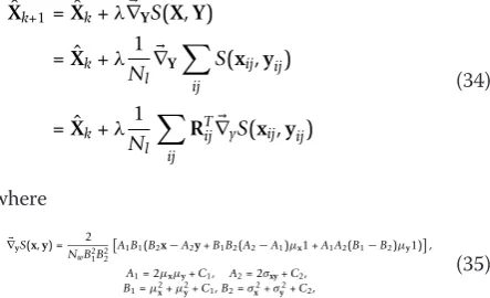
Peppers, House. It also compares the K-SVD method [3] with the proposed denoising method. It can be observed that the proposed denoising method achieves better per-formance in terms of SSIM which is expected to imply better perceptual quality of the denoised image. Figures 2 and 3 show the denoised images using K-SVD [3] and the proposed methods along with corresponding SSIM maps. It can be observed that SSIM-based method out-performs specially in the texture region which confirms that the proposed denoising scheme preserves the struc-tures better and therefore has better perceptual image quality.
3.2 Image super-resolution
In this section we demonstrate the performance of the SSIM-based sparse representations when used for image super-resolution. In this problem, a low resolution image,Y, is given and a high resolution version of the image,X, is required as output. We assume that the low resolution image is produced from high resolution image based on the following equation:
Y=DHX, (37)
where H represents a blurring matrix, and D is a
downsampling matrix. We use local sparsity model as prior to regularize this problem that has infinite many solutions which satisfy (37). Our approach is motivated by recent results in sparse signal representation, which suggests that the linear relationships among high-resolu-tion signals can be accurately recovered from their low-dimensional projections. Here, we work with two coupled dictionaries,Ψhfor high-resolution patches, and
Ψl for low-resolution ones. The sparse representation of a low-resolution patch in terms of Ψl will be directly used to recover the corresponding high resolution patch fromΨh[20]. Given these two dictionaries, each
resolution image,x, can be represented sparsely with the same coefficient vector,ain Algorithm 2.
y=lα (38)
x=hα (39)
The patch from each location of the low-resolution image, that needs to be scaled up, is extracted and spar-sely coded with the help of SSIM-optimal Algorithm 1. Once the sparse coefficients,a, are obtained, high
reso-lution patches, y, are computed using (39) which are
finally merged by averaging in the overlap area to create the resulting image. The proposed image super-resolu-tion algorithm is summarized in Algorithm 3:
The proposed image super resolution scheme is tested on various images. To be consistent with [20] patches of 5 × 5 pixels were used on the low resolution image. Each patch is converted to a vector of length 25. The dictionaries are trained using KSVD [3] with the sizes of 25 × 1024 and 100 × 1024 for the low and the high resolution dictionaries, respectively. 66 natural images are used for dictionary training, which are also used in [43] for similar purpose. To remove artifacts on the patch edges we set overlap of one pixel during patch extraction from the image. Fixed number of atoms (3) has been used by [20] in the sparse coding stage. How-ever SSIM-OMP determines the number of atoms adap-tively from patch to patch based on its importance considering SSIM measure. In order to calculate the Table 1 SSIM and PSNR comparisons of image denoising results
Image Barbara Lena Peppers House
Noise std 20 25 50 100 20 25 50 100 20 25 50 100 20 25 50 100
PSNR comparison (in dB)
Noisy 22.11 20.17 14.15 8.13 22.11 20.17 14.15 8.13 22.11 20.17 14.15 8.13 22.11 20.17 14.15 8.13 K-SVD 30.85 29.55 25.44 21.65 32.38 31.32 27.79 24.46 30.80 29.72 26.10 21.84 33.16 32.12 28.08 23.54 Proposed 30.88 29.53 25.50 21.74 32.26 31.28 27.80 24.53 30.84 29.84 26.25 21.98 33.04 32.09 28.13 23.59
SSIM comparison
Noisy 0.593 0.503 0.241 0.084 0.531 0.443 0.204 0.074 0.529 0.442 0.212 0.076 0.452 0.368 0.166 0.057 K-SVD 0.894 0.859 0.708 0.519 0.903 0.877 0.733 0.550 0.905 0.883 0.782 0.601 0.909 0.890 0.779 0.549 Proposed 0.906 0.875 0.733 0.526 0.913 0.888 0.754 0.573 0.913 0.894 0.797 0.627 0.915 0.901 0.795 0.574
(a)
(b)
(c)
(d)
(e)
(f)
(g)
threshold,Tssim, defined in (14),Tmseis calculated using
MSE-based sparse coding stage in [20]. After calculating sparse representation for all the low resolution patches, we use them to reconstruct the patches and then the difference with the original patch is calculated. We set Tmse to the average of these differences. The
perfor-mance comparison with state-of-the-art method is given in Table 2. It can be observed that the proposed algo-rithm outperforms the other methods consistently in terms of SSIM evaluations. It is also interesting to observe PSNR improvements in some cases, though PSNR is not the optimization goal of the proposed approach. The improvements are not always consistent (for example, PSNR drops in some cases in Table 1, while SSIM always improves). There are complicated reasons behind these results. It needs to be aware that
the so-called “MSE-optimal” algorithms include many
suboptimal and heuristic steps and thus have potentials to be improved even in the MSE sense. Our methods are different from the“MSE-optimal” methods in multi-ple stages. Although the differences are made to improve SSIM, they may have positive impact on improving MSE as well. For example, when using the learned dictionary to reconstruct an image patch, if SSIM is used to replace MSE in selecting the atoms in the dictionary, then essentially the set of accepted atoms in the dictionary have been changed. In particular, since SSIM is variance normalized, the set of acceptable reconstructed patches near the noisy patch may be structurally similar but are significantly different in var-iance. This may lead to different selections of the atoms in the dictionary, which when appropriately scaled to approximate the noisy patch, may result in better recon-struction result. Although the visual and SSIM
(a)
(b)
(c)
(d)
(e)
(f)
(g)
Figure 3Visual comparison of denoising results.(a)Original image;(b)noisy image;(c)SSIM-map of noisy image;(d)KSVD-MSE;(e) SSIM-map of KSVD-MSE;(f)KSVD-SSIM;(g)SSIM-map of KSVD-SSIM.
Table 2 SSIM and PSNR comparisons of image super-resolution results
Image Barbara Lena Baboon House Raccoon Zebra Parthenon Desk Aeroplane Man Moon Bridge
PSNR comparison (in dB)
Yang et al. 30.3 33.4 25.3 34.1 34.0 24.6 28.4 31.9 34.2 33.2 32.2 28.0 Zeyde et al. 31.3 33.8 25.5 35.4 36.5 25.0 28.8 33.8 36.1 34.4 33.3 28.5 Proposed 31.4 33.9 25.6 35.5 37.0 25.1 28.9 33.9 36.4 34.6 33.4 28.6
SSIM comparison
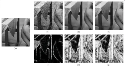
improvements are only moderate, these are promising results as an initial attempt of incorporating a percep-tually more meaningful measure into the optimization problem of KSVD-based superresolution method. Fig-ures 4 and 5 compare the reconstructed images obtained using [5] and the proposed methods for the Raccoon and the Girl images, respectively. It can be seen that the proposed scheme preserves many local structures better and therefore has better perceptual image quality. The visual quality improvement is also reflected in the corresponding SSIM maps, which pro-vide useful guidance on how local image quality is improved over space. It can be observed from the SSIM maps that the areas which are relatively more structured benefit more from the proposed algorithm as the quality measure used is better at calculating the similarity of structures as compared to MSE.
4 Conclusions
In this article, we attempt to combine perceptual image fidelity measurement with optimal sparse signal repre-sentation in the context of image denoising and image
super-resolution to improve two state-of-the-art algo-rithms in these areas. We proposed an algorithm to solve for the optimal coefficients for sparse and redun-dant dictionary in maximal SSIM sense. We also devel-oped a gradient descent approach to achieve the best compromise between the distorted image and the image reconstructed using sparse representation. Our simula-tions demonstrate promising results and also indicate the potential of SSIM to replace the ubiquitous PSNR/ MSE as the optimization criterion in image processing applications. It must be taken into account that this is only an early attempt along a new but promising direc-tion. The main contribution of the current work is mostly in the general framework and theoretical devel-opment. Significant improvement in visual quality can be expected by improving the dictionary learning pro-cess based on SSIM, as dictionary encapsulates in itself the prior knowledge about the image to be restored. An SSIM-optimal dictionary will capture structures con-tained in the image in a better way and the restoration task will result into sharper output image. Further improvement is also expected in the future when some
(a)
(b)
(c)
(d)
(e)
(f)
of the advanced mathematical properties of SSIM and normalized metrics [12] are incorporated into the opti-mization framework.
Algorithm 1: SSIM-inspired OMP
Initialize:D= {} set of selected atoms,Sopt = 0,r=Y while Sopt<Tssim
•Add the next best atom in L2 sense toD
•Find the optimal L2-based coefficient(s) using (15)
• Find the optimal SSIM-based coefficient(s) using
(27) and (31)
•Update the residualr
•Find SSIM-based approximationa
•CalculateSopt=S(a, y)
end
Algorithm 2: SSIM-inspired image denoising 1.Initialize:X =Y,Ψ= overcomplete DCT dictionary
2.Repeat J times
• Sparse coding stage: use SSIM-optimal OMP to compute the representation vectors aijfor each patch
•Dictionary update stage: Use K-SVD [28] to calcu-late the updated dictionary and coefficients. Calculate
SSIM-optimal coefficients using (27) and (31)
3.Global Reconstruction: Use gradient descent algo-rithm to optimize (6), where the SSIM gradient is given by (35).
Algorithm 3: SSIM-inspired image super resolution
1.Dictionary Training Phase:trained high and low reso-lution dictionariesΨl,Ψh, [20]
2.Reconstruction Phase
•Sparse coding stage: use SSIM-optimal OMP to compute the representation vectorsaijfor all the patches
of low resolution image
•High resolution patches reconstruction:Reconstruct high resolution patches byΨhaij
3. Global Reconstruction: merge high-resolution patches by averaging over the overlapped
region to create the high resolution image.
(a)
(b)
(c)
(d)
(e)
(f)
Acknowledgements
This work was supported in part by the Natural Sciences and Engineering Research Council of Canada and in part by Ontario Early Researcher Award program, which are gratefully acknowledged.
Author details
1Department of Electrical and Computer Engineering, University of Waterloo, Waterloo, ON, N2L 3G1 Canada2Department of Applied Mathematics, University of Waterloo, Waterloo, ON, N2L 3G1 Canada
Competing interests
The authors declare that they have no competing interests.
Received: 6 June 2011 Accepted: 20 January 2012 Published: 20 January 2012
References
1. K Dabov, A Foi, V Katkovnik, K Egiazarian, Image denoising by sparse 3D transform-domain collaborative filtering. IEEE Trans. Image Process.16, 2080–2095 (2007)
2. A Buades, B Coll, JM Morel, A review of image denoising algorithms, with a new one. Multi-scale Model Simul.4(2), 490–530 (2005). doi:10.1137/ 040616024
3. M Elad, M Aharon, Image denoising via sparse and redundant
representations over learned dictionaries. IEEE Trans Image Process.15(12), 3736–3745 (2006)
4. H Hou, H Andrews, Cubic splines for image interpolation and digital filtering. IEEE Trans Signal Process.26, 508–517 (1978). doi:10.1109/ TASSP.1978.1163154
5. J Yang, J Wright, T Huang, Y Ma, Image super-resolution via sparse representation. IEEE Trans Image Process.19(11), 2861–2873 (2010) 6. J Yang, J Wright, TS Huang, Y Ma, Image super-resolution as sparse representation of raw image patches. inProc IEEE Comput Vis Pattern Recognit1–8 (2008)
7. Z Wang, AC Bovik, Mean squared error: love it or leave it? A new look at signal fidelity measures. IEEE Signal Process Mag.26, 98–117 (2009) 8. Z Wang, AC Bovik, HR Sheikh, EP Simoncelli, Image quality assessment:
from error visibility to structural similarity. IEEE Trans Image Process.13(4), 600–612 (2004). doi:10.1109/TIP.2003.819861
9. Joint Video Team (JVT) Reference Software [Online], http://iphome.hhi.de/ suehring/tml/download/old_jm
10. Y Gao, A Rehman, Z Wang, CW-SSIM Based image classification, inIEEE International Conference on Image Processing ICIP, Brussels, Belgium, pp. 1249–1252 (2011)
11. G Piella, H Heijmans, A new quality metric for image fusion, inIEEE International Conference on Image Processing (ICIP), vol. 3. Barcelona, Spain, pp. 173–176 (2003)
12. D Brunet, ER Vrscay, Z Wang, in On the Mathematical Properties of the Structural Similarity Index (Preprint), University of Waterloo, Waterloo, 2011 http://www.math.uwaterloo.ca/~dbrunet/
13. SS Channappayya, AC Bovik, C Caramanis, R Heath, Design of linear equalizers optimized for the structural similarity index. IEEE Trans Image Process.17(6), 857–872 (2008)
14. Z Wang, Q Li, X Shang, Perceptual image coding based on a maximum of minimal structural similarity criterion. IEEE Int Conf Image Process.2, II-121–II-124 (2007)
15. A Rehman, Z Wang, SSIM-based non-local means image denoising, inIEEE International Conference on Image Processing (ICIP), Brussels, Belgium, pp. 1–4 (2011)
16. S Wang, A Rehman, Z Wang, S Ma, W Gao, Rate-SSIM optimization for video coding, inIEEE International Conference on Acoustics Speech and Signal Processing (ICASSP 11), Prague, Czech Republic, pp. 833–836 (22–27 May 2011) 17. T Ou, Y Huang, H Chen, A perceptual-based approach to bit allocation for
H.264 encoder, inSPIE Visual Communications and Image Processing, pp. 77441B (11 July 2010)
18. Z Mai, C Yang, K Kuang, L Po, A novel motion estimation method based on structural similarity for h.264 inter prediction, inIEEE Int Conf Acoust Speech Signal Process, vol. 2. (Toulouse, 2006), pp. 913–916
19. C Yang, H Wang, L Po, Improved inter prediction based on structural similarity in H.264, inIEEE Int Conf Signal Process Commun, vol. 2. Dubai, pp. 340–343 (24–27 Nov 2007)
20. R Zeyde, M Elad, M Protter, On single image scale-up using sparse-representations, inCurves & Surfaces, Avignon-France, pp. 711–730 (24–30 June 2010)
21. A Savitzky, MJE Golay, Smoothing and differentiation of data by simplified least squares procedures. Anal Chem.36, 1627–1639 (1964). doi:10.1021/ ac60214a047
22. AN Tikhonov, VY Arsenin,Solutions of Ill-Posed Problem(V. H. Winston, Washington DC, 1977)
23. LI Rudin, S Osher, E Fatemi, Nonlinear total variation based noise removal algorithms. Physica D.60, 259–268 (1992). doi:10.1016/0167-2789(92)90242-F 24. M Protter, M Elad, Image sequence denoising via sparse and redundant
representations. IEEE Trans Image Process.18, 27–35 (2009)
25. J Mairal, G Sapiro, M Elad, Learning multiscale sparse representations for image and video restoration. Multiscale Model Simul.7, 214–241 (2008). doi:10.1137/070697653
26. EJ Candés, J Romberg, T Tao, Robust uncertainty principles: exact signal reconstruction from highly incomplete frequency information. IEEE Trans Inf Theory.52(2), 489–509 (2006)
27. DL Donoho, Compressed sensing. IEEE Trans Inf Theory.52(4), 1289–1306 (2006)
28. M Aharon, M Elad, A Bruckstein, K-SVD: an algorithm for designing overcomplete dictionaries for sparse representation. IEEE Trans Signal Process.54(11), 4311–4322 (2006)
29. Y Pati, R Rezaiifar, P Krishnaprasad, Orthogonal matching pursuit: recursive function approximation with applications to wavelet decomposition, in Twenty Seventh Asilomar Conference on Signals, Systems and Computers, vol. 1. Pacific Grove, CA, pp. 40–44 (Nov 1993)
30. D Brunet, ER Vrscay, Z Wang, Structural similarity-based approximation of signals and images using orthogonal bases, inProc Int Conf on Image Analysis and Recognition, ed. by M Kamel, A Campilho (Springer, Heidelberg, 2010), pp. 11–22. vol. 6111 of LNCS
31. S Wang, A Rehman, Z Wang, S Ma, W Gao, SSIM-inspired divisive normalization for perceptual video coding, inIEEE International Conference on Image Processing ICIP, Brussels, Belgium, pp. 1657–1660 (11–14 Sept 2011)
32. MJ Wainwright, EP Simoncelli, Scale mixtures of gaussians and the statistics of natural images. Adv Neural Inf Process Syst.12, 855–861 (2000) 33. S Lyu, EP Simoncelli, Statistically and perceptually motivated nonlinear
image representation, inProc SPIE Conf Human Vision Electron Imaging XII, vol. 6492. San Jose, CA, pp. 649207-1–649207-15 (2007)
34. J Foley, Human luminance pattern mechanisms: masking experiments require a new model. J Opt Soc Am.11, 1710–1719 (1994). doi:10.1364/ JOSAA.11.001710
35. AB Watson, JA Solomon, Model of visual contrast gain control and pattern masking. J Opt Soc Am.14, 2379–2391 (1997). doi:10.1364/JOSAA.14.002379 36. DJ Heeger, Normalization of cell responses in cat striate cortex. Vis Neural
Sci.9, 181–198 (1992)
37. EP Simoncelli, DJ Heeger, A model of neuronal responses in visual area MT. Vis Res.38, 743–761 (1998). doi:10.1016/S0042-6989(97)00183-1
38. Q Li, Z Wang, Reduced-reference image quality assessment using divisive normalization-based image representation. IEEE J Coupled dictionary training for image s Spec Top Signal Process.3, 202–211 (2009) 39. A Rehman, Z Wang, Reduced-reference SSIM estimation, inInternational
Conference on Image Processing, Hong Kong, China, pp. 289–292 (27–29 Sept 2010)
40. J Malo, I Epifanio, R Navarro, EP Simoncelli, Non-linear image representation for efficient perceptual coding. IEEE Trans Image Process.15, 68–80 (2006) 41. J Portilla, V Strela, MJ Wainwright, EP Simoncelli, Image denoising using
scale mixtures of Gaussians in the wavelet domain. IEEE Trans Image Process.12, 1338–1351 (2003). doi:10.1109/TIP.2003.818640 42. Z Wang, EP Simoncelli, Maximum differentiation (MAD) competition: a
methodology for comparing computational models of perceptual quantities. J Vis.8(12), 1–13 (2008). doi:10.1167/8.12.1
43. J Yang, Z Wang, Z Lin, T Huang, Coupled dictionary training for image super-resolution. http://www.ifp.illinois.edu/~jyang29/ (2011)
doi:10.1186/1687-6180-2012-16
Cite this article as:Rehmanet al.:SSIM-inspired image restoration using sparse representation.EURASIP Journal on Advances in Signal Processing