R E S E A R C H
Open Access
Evaluation of the modified
S
-transform for
time-frequency synchrony analysis and source
localisation
Said Assous
1*and Boualem Boashash
2,3Abstract
This article considers the problem of phase synchrony and coherence analysis using a modified version of theS -transform, referred to here as the ModifiedS-transform (MST). This is a novel and important time-frequency approach to study the phase coupling between two or more different spatially recorded entities with stationary characteristics. The basic method includes a cross-spectral analysis to study the phase synchrony of non-stationary signals, and relies on some properties of the MST, such as phase preservation. We demonstrate the usefulness of the technique using simulated examples and real newborn EEG data. The results show the advantage of using the cross-MST in the study of the connectivity between different signals using the time-frequency
coherence. The MST led to improvements in resolution of almost twofold over the standardS-Transform in the examples presented in the article.
Keywords:time-frequency coherence, cross time-frequency, modifiedS-transform, phase synchrony, array proces-sing, EEG signal, time-frequency signal analysis, Quadratic Time-Frequency Distributions, instantaneous frequency
1 Introduction
1.1 Time-frequency methods
Non-stationary signals have statistical properties that vary with time and hence the traditional time averaged amplitude spectrum obtained using Fourier transform is inadequate to track changes in signal magnitude, fre-quency or phase. In analyzing non-stationary and multi-component signals, time-frequency-based techniques were shown to outperform classical techniques based on either time or frequency domains [1] (Chapter 1). The basic idea of time-frequency analysis is to understand and describe situations where the frequency content of a signal is changing in time. Although time-frequency analysis had its origin almost 50 years ago, significant advances have occurred in the past 20 years or so. In particular, the time-frequency representation has received considerable attention as a powerful high reso-lution and precision tool for analyzing a variety of bio-signals and systems such as speech, ECG, EEG, PCG, EMG, as well as signals arising from other fields [2]. A
time-frequency distribution (TFD) is used to analyze and process non-stationary signals in the joint time-fre-quency domain. Several TFDs exist in the literature [1]. Most of them are based on the Wigner-Ville distribution (WVD) [3], as all the other TFDs can be expressed as a smoothed version of the WVD. A popular candidate of this class is the spectrogram, which is the square modu-lus of the short time Fourier transform (STFT). The spectrogram is the WVD smoothed in time and fre-quency by the ambiguity function of the window used in the STFT [4]; and all the quadratic TFDs (QTFD) are 2D-smoothed versions of the WVD (and therefore of the spectrogram which is the square modulus of the STFT). The spectrogram has been widely used as an initial investigative tool [1] as it has the property of being a cross-terms free TFD; but it also suffers from the undesirable trade-off between time concentration and frequency concentration. To address the problem of cross-terms suppression, while keeping a high time-fre-quency resolution, other TFDs have been proposed. Among these, one can cite the smoothed pseudo WVD (SPWVD) [1], the Cone shaped kernel TFD (ZAMD) [5], Gaussian TFD [6] and the Modified B-distribution * Correspondence: [email protected]
1Weatherford, East Leake, Leicestershire LE12 6JX, UK
Full list of author information is available at the end of the article
(MBD) [1] (Chapter 3) just to name a few. These meth-ods form a class commonly referred to as QTFDs or Bilinear TFDs, as they represent and distribute the energy of a signal in the time-frequency domain. A dif-ferent method, the continuous wavelet transform (CWT) has a wide area of application and can be seen as an extension of the spectrogram in a wide sense, except for representing signals in time-scale space instead of time-frequency space. As it is linear and based on amplitude decomposition, it is also a useful technique for filtering in the time-scale space. A more recently developed method called S-transform (ST) is conceptually a hybrid of the STFT and CWT. The ST uses a variable analyzing window length but preserves the phase information by using a Fourier kernel in the signal decomposition [7].
The above indicates that various methods of perform-ing a time-frequency analysis exist. No method is super-ior to another, since they all have benefits for specific types of signals and applications to which they are adapted, depending on signal characteristics such as spectral contents.
The novel contributions in this article are mostly based on
•The design of the modified ST (a signal-dependent version of the standard ST with an improved time-frequency resolution).
• The design and application of the cross-modified ST to investigate the phase synchrony between sig-nals in the time-frequency plane and source location.
1.2 Phase synchrony and source location
Phase synchrony analysis is a useful measure of linear dependence between two stochastic signals. This approach is based on the concept of phase synchroniza-tion of chaotic oscillators studied by Rosenblum et al. [8]. The phase synchrony (coefficient) takes on values between 0, for two signals at different frequencies, and 1, for signals that exhibit a constant difference in instan-taneous phase (representing the situation where a signal and its time-shifted version are observed). So, phase syn-chrony refers to the interdependence between the instantaneous phases of two signals; the instantaneous phases may be strongly synchronized even when the amplitudes of the two signals are statistically indepen-dent [8]. Estimating this measure requires pre-filtering at a frequency of interest. The interesting properties of the phase synchrony coefficient are its independence of the signal amplitudes and that no assumptions about the nature of the signals are made. Another useful mea-sure of linear dependence between two stochastic signals is the coherence function, which quantifies linear
linear in time for sinusoidal signals, and can thus be applied for phase synchrony. Although the wavelet and STFT-based phase synchrony approaches consider the nonstationarity issue, they suffer from a number of drawbacks. In the case of the wavelet transform, where we have a progressive time-frequency resolution the estimate won’t be the same for the whole bandwidth of the signal, which means a non uniform time-frequency tiling on the analyzed signal and thus results in biased energy representations and corresponding phase esti-mates. In the case of STFT, there is a trade-off between time and frequency resolution due to the window func-tion. For these reasons, there is a need for a higher time-frequency resolution phase distributions that can track dynamic changes in phase synchrony over the whole time-frequency plane. As cited above, and given a measurements made from an array of electrodes or sen-sors, phase synchronization methods are used to detect the phase difference between two signals from two dif-ferent electrodes or sensors, this can be applied for source location. First, appropriate neighborhood of each channel or electrode is constructed. Then phase syn-chronization is measured between the channel and each neighbor. Only those channels have been identified as closest to the potential sources where strong phase syn-chronization is detected will be considered for source location.
The article is organized as follow: The Section 2 intro-duces the ST definition, its key properties and provides a brief comparison between ST, CWT, and QTFD will be also reviewed. The Section 3 presents the concept and formulation of generalized ST and shows the improved resolution using the modified ST on synthetic examples. The Section 4 discusses the Cross-MST for time-frequency coherence analysis on synthetic exam-ples. The Section 5 demonstrates the application of the cross-MST for phase synchrony detection to simulated EEG seizure and real newborn EEG data.
2 Advantages and limitations of the ST
The advent of time-frequency analysis techniques using QTFDs, STFT, and wavelet transforms made the analy-sis of non-stationary signals more precise. The low reso-lution of the STFT and the absence of phase information in the CWT led to the development of the ST, which has the property of retaining the absolute phase information, while preserving a good time-fre-quency resolution for all frequencies. Even though the ST has better time-frequency resolution compared to STFT, the resolution is far from perfect and needs improvement. The CWT uses a basis function which dilates and contracts with frequency; it does not retain the absolute phase information; further, the visual analy-sis of the time-scale plots that are produced by the
CWT is intricate. The ST combines the good features of STFT and CWT and can be viewed either as a variable sliding window STFT or as a phase-corrected CWT [7], as detailed below.
2.1 Definition and key relationships
Given a time seriesx(t), the local spectrum at timet=τ can be determined by multiplying x(t) with a Gaussian window located at t= τand taking the Fourier trans-form of the product. This defines the ST as follows: [7]
S(t,f,σ) =
+∞
−∞
x(τ)g(t−τ,σ)e−j2πfτdτ (1)
The original ST usesg(t- τ,s) as the scaled Gaussian window whose midpoint isτ=t. At any timetand fre-quencyf, the ST can be seen as a set of localised Fourier coefficients, obtained by considering only the portion of the primary function lying within a few cycles on either side ofτ =t. The scaled contraction ofg(t-τ,s) causes the relevant range ofτ to become more localised around tasfincreases.
g(t−τ,σ) = √1 2πσe
−(t−τ)2
2σ2 (2)
If we selectσ = |1f|, Equation (2) becomes
g(t−τ, 1/f) = √f 2πe
−(t−τ)2f2
2 (3)
and its Fourier transform with respect toτ (which is gaussian as well) becomes
G(ν,f) =e −2π2ν2
f2 (4)
By choosingσ =|1f|makesg(t- τ,s) with two control parameters rather than three and add some constraints to the frequency. Hence, the ST can be defined as an adaptative STFT or as a CWT with a specific mother wavelet-like term multiplied by a phase factor.
S(t,f) =e−j2πftWT(t,d) (5) where the scale factor dis inversely proportional to the frequencyfand
WT(t,d) =
+∞
−∞
x(τ)g(t−τ,d)dτ (6)
g(t−τ,f) = √f 2πe
−−f2(t2−τ)2e−j2πf(t−τ) (7)
The ST separates the mother wavelet-like into two parts, the slowly varying envelope (the Gaussian func-tion) which localises in time the amplitude modulated (AM) component, and the oscillatory exponential kernel e-j2πfτ which selects the frequency being localised, the frequency modulated (FM) component. Hence, this separate AM-FM decomposition is similar in concept to the empirical mode decomposition (EMD), which is a local and fully data-driven technique aimed at decom-posing non-stationary multicomponent signals in “intrinsic”AM-FM contributions [15]. The ST analyzing window is actually not a mother wavelet in a strict sense. It is the time localizing Gaussian parameter that is translated while the oscillatory exponential kernel remains stationary. By not translating the oscillatory exponential kernel in Equation (7), the ST localises the real and the imaginary components of the spectrum independently, therefore localizing the phase spectrum as well as the amplitude spectrum. This is referred to as absolutely referenced phase information [7]. Unlike the CWT, the ST produces a time-frequency representation instead of a time-scale representation.
2.2 The ST and signal spectrum
Integrating the ST over time results in the Fourier transform. This direct relation to the Fourier transform and the linearity property of the ST make both the inversion to time domain and the filtering process in the time-frequency domain possible. The ST is thus a representation of local spectrum; The relationship between the ST and the signal spectrum X(f) can be expressed as follows:
+∞
−∞
S(t,f)dt=X(f) (8)
whereX(f) is the Fourier transform of x(t). Hence,x(t) can be retrieved from ST by:
x(t) =
+∞
−∞ ⎧ ⎨ ⎩
+∞
−∞
S(t,f)dt ⎫ ⎬
⎭ej2πftdf (9)
This relationship shows that the concept of the ST is different from both the wavelet transform and QTFDs. The concept of recovering back the signal from the ST time-frequency plane is due to the fact that the phase is referenced at the origin, which means that the phase information given by the ST refers to the argument of the cosinusoid at zero time as it is the case for Fourier transform. In contrast, The phase spectrum of the signal
can be extracted from its wavelet transform CWT, as a convolution of the signal with a complex wavelet, where the phase of the CWT is relative to the center (in time) of the analyzing wavelet (the mother wavelet). Thus as the wavelet translates, the reference point of the phase translates giving a locally referenced phase which is dis-tinguishable from the phase properties of the ST and the signal can’t be recovered from the time-scale plane. On the other hand, the fact that QTFDs are bilinear and real valued energy distributions describing the energy of the signal over time and frequency, simultaneously, they cannot be used for estimating the phase of an individual signal and the phase synchrony between two signals. Moreover, the inverse process also is not straightfor-ward, as it requires some initial conditions.
The relation between the ST and the signal spectrum X(f) is given in [7] and can be written as
S(t,f) =
+∞
−∞
X(ν+f)e−
2π2ν2
f2
ej2πνtdν, f = 0 (10)
The equivalent discrete version of Equation (10) can be used to compute the discrete ST by taking advantage of the computational efficiency of the fast Fourier trans-form (FFT) and the convolution theorem.
2.3 Comparison of ST, CWT, and QTFDs
The similarities and differences between the ST, CWT, and QTFDs are reviewed below.
(1) ST and Morlet wavelet: Although the differences between the ST and Morlet wavelet are suitable, the only difference between ST and Morlet wavelet decom-position is that the ST time-frequency function is scaled by the carrier frequencyf. Additionally, the amplitude modulation term fsmoothes the ST spectrum, but may cause computational artifacts in the Morlet spectrum at low frequencies. Furthermore, the phase correction term in ST enable the ST to preserve absolute referenced phase information of a signal. Also, ST approach has advantages over the Morlet wavelet approach in terms of easy interpretation and fast computation.
(3)Invertibility and recoverable signal parameters: As the ST output is complex, we can read the amplitudeA (t) = abs(S(t, f)), the frequency f, and the phase
informa-tionφ(t) = atan
Im (S(t,f)) Re (S(t,f))
for each time step from
the ST. This allows us to extract the corresponding nal by reproducing it in the time domain as follows: sig-nal(t) = A(t)cos(2πf(t)t+j(t)). The signal parameters were recoverable due to the combination of absolutely referenced phase information and frequency invariant amplitude of the ST, and such direct extraction cannot be done with CWT-based method. Moreover, the direct measurement of phase information makes the ST a potential candidate to estimate the phase synchrony between two signals.
For QTFDs, a signal x(t) can be recovered exactly, apart from a complex scaling factor [1, p. 61].
(4) ST phase: The ST retains the absolute phase information, where as the phase information is lost in the CWT. The absolutely referenced (at time t = 0) phase of the ST leads to a generalization of the instan-taneous frequency to broadband signals and can be used as a local peak-finding algorithm [16,17], for example. In contrast, in the wavelet approach; the phase is relative to the center (in time) of the analyz-ing wavelet, and as the wavelet translates, the reference point of the phase translates, hence the relative phase becomes meaningless. With the ST, the sinusoidal component of the basis function remains stationary, while the Gaussian envelope translates in time. Thus, the reference point for the phase remains stationary and the phase has the same meaning as in the Fourier domain [18]. For QTFDs, the phase information is linked to the time delay or instantaneous frequency [12]. The phase information can be extracted using the cross-WVD or related methods [19].
(5)ST amplitude:The time domain localizing window (the Gaussian function) in Equation (7) is normalized by the factor|f|
2π to the unit area. In contrast to the CWT,
this makes the amplitude response of the ST invariant to the frequency, which means that for a sinusoid with an amplitudeA(x(t) =Acos(2πft)), the ST returns an amplitude Aregardless of the frequency f in a similar concept as the amplitude of the Fourier transform. On the other hand, the amplitude of the CWT is large for the lower frequencies and diminishes at the higher fre-quency components. This lower amplitude estimation at the high frequencies is mainly due to the normalization of the CWT [18]. For QTFDs, it is the signal energy that is distributed in tand f, not the signal amplitude. Hence, the interpretation is different. The spectrogram is the square modulus of the STFT; and as the QTFDS are a 2D convolution of the spectrogram, the spectrum
X(f) can also be recovered subject to the initial complex constantX(f= 0).
(6)Cross-ST analysis: As the ST is complex and its phase characteristic is referenced at the origin, it can be employed in a cross spectrum analysis in a local manner to estimate the phase synchrony between two signals. Consider two signals measured by two receivers (trans-ducers) separated by a known distance. Let a sinusoidal wave propagate through the medium of view of both receivers. What we will get is the same signal in both sensors with an additive noise (assuming a controlled environment conditions), but also with a time shift between the two signals. Since the ST is a linear opera-tion on the signal and localizes spectral components in time, the cross correlation of specific events on two spa-tially separated STs will give the phase difference, hence the time delay between the two signals can be measured [18]. This concept is also found in cross-TFDs using quadratic methods, where the signal and its complex conjugate are used to calculate the cross-spectrum [19].
(7) Co-ST and quadrature-ST: As the local phase information can be extracted from the ST, we can use the cross-ST function to analyze the in-phase and the out-of-phase components in time-frequency space. This is a very useful characteristic for cross-spectral and phase synchrony. This property is exploited later for an array of EEG signals to estimate the phase synchrony between signals recorded from different electrodes and assess the source location of the brain activities. The cross-ST phase can be used to analyze this synchrony or asynchrony, thus providing a significant discriminating feature for potential abnormal brain activity. As with classical co-spectrum analysis, the real part of the cross-ST function gives the in-phase components of the local spectra. The imaginary part of the cross-ST function gives the in-quadrature components. This property is discussed in detail in Section 3.
The above paragraphs indicate that, unlike the QTFDs, the ST is linear with progressive resolution (see Section 3.3.2 for more details). Unlike the CWT and STFT, the ST has a variable analysis window and an absolute phase reference. These useful properties of the ST make it a natural candidate to study the phase syn-chrony between two different spatially recorded signals.
2.4 Limitations of the ST
The ST was defined with two unnecessary restrictions on the window function detailed below.
• Firstly, only a Gaussian window g(t, s) is considered.
• Also, that window has no parameters to allow its width in time or frequency to be adjusted, as shown in Equation (2).
The resolution, on the ST, of the onset times of events can be improved by using a narrower window, for example, using a better controlled parameters of the Gaussian window. However, when a window is nar-rowed in the time domain, it inevitably widens in the frequency domain, with consequent loss of resolution in the frequency direction on the ST compromising the identification of the whole event. One way of addressing this problem is to use extra parameters controlling the scale and the shape of the analyzing window rather than just only making the frequency inversely proportional to the standard deviations.
3 Extension of the ST for resolution improvement
3.1 Concept and definition
To remedy the limitations discussed in the previous sec-tion, a variant of the original ST, introduced by Man-sinha et al. [20], replaces f with γf in Equation (7). By doing this, one standard deviation of the Gaussian win-dow contains g wavelengths of the Fourier sinusoid at all frequencies. This allows a better control of the time and frequency resolution of the ST on the time-fre-quency plane. More recently, McFadden et al. [21] pre-sented a generalized ST which includes windows which are asymmetrical. They applied an asymmetrical window to analyze gearbox vibration signals. Later on, Pinnegar and Mansinha [22] have extended the generalization idea in [21] of the ST to include windows which have complicated scaling properties, including frequency-dependent shape and applied this approach to a broad-band earthquake seismogram contaminated by noise. This generalized form retains the property of invertibil-ity of the originalS-transform [7] and its relation to the Fourier spectrum. The generalized ST is parameterized by a width control adjustment coefficientg; it is given by
S(t,f,γ) =
+∞
−∞
x(τ)g(t−τ,f,γ)e−j2πfτdτ (11)
where g(t- τ, f,g) is the generalized window function of the ST and g denotes the set of parameters that determine the shape and the properties of the window function, and the parameter tcontrols the position of the generalized window on the time axis. The Gaussian window is given by
g(t−τ,f,γ) = f γ√2πe
−f2(t−τ)2
2γ2 (12)
Note that, as in Equation (10), the generalized ST can also be obtained from the signal spectrum as shown below.
S(t,f,γ) =
+∞
−∞
X(ν+f)G(ν,f,γ)ej2πνtdν (13)
3.2 Key properties
The generalized window g(t- τ, f, g) satisfies the follow-ing normalization criteria,
+∞
−∞g(t−τ,f,γ)dt= 1 (14)
This ensures that the time averaging of the ST spec-trumS(t, f,g) yields the spectrum X(f), as shown in (15) below
+∞
−∞
S(t,f,γ)dt=
+∞
−∞
+∞
−∞
x(τ)g(t−τ,f,γ)e−j2πfτdτdt (15)
=
+∞
−∞
x(τ)e−j2πfτ
+∞
−∞
g(t−τ,f,γ)dtdτ (16)
=
+∞
−∞
x(τ)e−j2πfτdτ =X(f) (17)
whereX(f) is the Fourier transform of the signalx(t).
3.3 Modified ST
3.3.1 Formulation of the modified ST
Based on this generalized form, we can examine the Gaussian window at a different scaling rule [23,24]. This can be achieved by getting the scaling parameter g defined above to vary linearly with the frequency to get better progressive control of the window width as fol-lows
γ(f) =mf+k (18)
MST(t,f,m,k) =
+∞
−∞
x(τ)g(t−τ,f,m,k)e−j2πfτdτ (19)
where g(t-τ, f, m, k) denotes the window function of the modified ST (MST), given as follows
g(t−τ,f,m,k) = f (mf+k)√2πe
−f2(t−τ)2
2(mf+k)2 (20)
Using Equations (19) and (20), the modified ST is given by:
MST(t,f,m,k) = +∞
−∞
x(τ) f (mf+k)√2πe
−f2(t−τ)2
2(mf+k)2e−j2πfτdτ (21)
The MST also satisfies the normalization condition for ST window defined in Equation (14) and hence is
invertible.
+∞
−∞
f (mf+k)√2πe
−f2(t−τ)2
2(mf+k)2 dτ = 1 (22)
3.3.2 Improved resolution of the MST
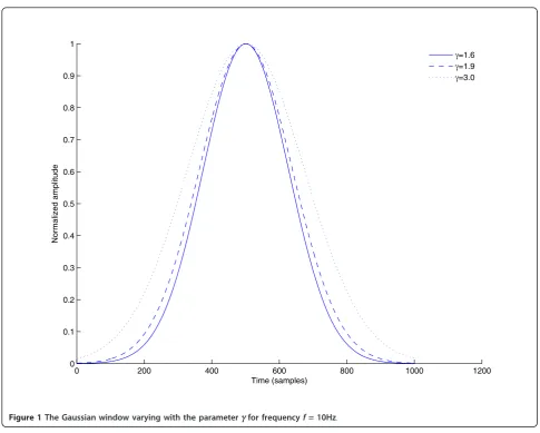
In a similar concept to [20], The parameterγf represents the number of cycles (periods) of a frequency that can be contained within one standard deviation s of the Gaussian window given by Equation (2). Hence, we have a progressive improved resolution in this case. When too small, the Gaussian window retains very few cycles of the sinusoid and the frequency resolution degrades at low frequencies. In contrast, if it is too large, the win-dow retains more cycles within it and in consequence, the time resolution degrades at high frequencies. This trade-off between time and frequency resolution is
0 200 400 600 800 1000 1200
0 0.1 0.2 0.3 0.4 0.5 0.6 0.7 0.8 0.9 1
Time (samples)
Normalized amplitude
=1.6 =1.9 =3.0
governed by the“Heisenberg” uncertainty principle in a similar way as in the FT, ST or the CWT.
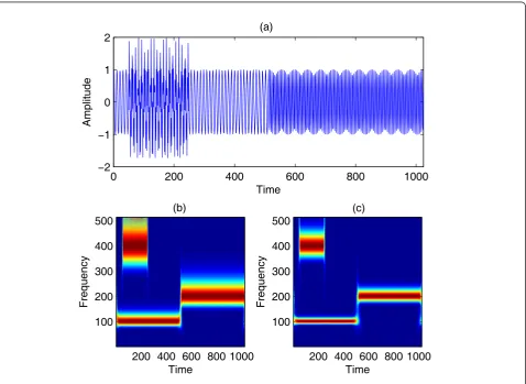
The value of mandkneed to be selected properly to get better resolution depending on the properties of the signal under consideration. Selected values of kequals to N1 andmequals to four times the variance of the sig-nal were found empirically to be appropriate; whereNis the length of the signal in samples. The method is therefore data dependent or adaptive. As an example for illustration, let’s consider a three components signal composed of: a low frequency (100Hz), medium fre-quency (200Hz) and a high frefre-quency burst (400Hz) as shown in Figure 2a. Figure 2b,c represent the ST and the MST, respectively, of the signal in Figure 2a.
Figure 2b,c show clearly the difference in time-fre-quency resolution when the ST and the MST are applied. Using the MST leads to an improvement of almost twofold in resolution over the ST.
3.3.3 Simulated results, discussion and interpretation In the previous example, the values of m and kwere chosen depending on the length and the variance of
the signal to get a better resolution (see Appendix 1 for more details). This indicates that as is the case with power spectral estimation, the approach is not restricted to a Gaussian window and any relevant win-dow or apodising function may be employed to improve resolution. The method is not restricted to a Gaussian window and can be generalized in a similar concept to the CWT for which different windows can be used. Hence, the ST can be seen as a special case of the CWT using a Morlet-type wavelet, with a phase and amplitude correction. This generalized form of ST is more flexible, as it uses two added parameters for varying the frequency in a linear way, resulting in adjustable windows for improved time or frequency resolution. Similar ideas led to the development of transforms based on groups generated by translations, modulations, and dilation of a mother wavelet [25]. All of these approaches give a more versatile choice of transform suitable to particular cases and applications. However, the particular characteristic of absolute phase, make the MST more attractive than wavelet
0 200 400 600 800 1000
−2
−1 0 1 2
Time
Amplitude
Frequency
Time
200 400 600 800 1000 100
200 300 400 500
Frequency
Time
200 400 600 800 1000 100
200 300 400 500
(c) (b)
(a)
when phase need to be estimated (e.g., in coherence analysis and cross-spectral analysis). It can simulta-neously estimate the local amplitude spectrum and the local phase spectrum, whereas a wavelet approach is only capable of probing the local amplitude/power spectrum. The MST fully estimates the amplitude of the signal, in contrast to the CWT which attenuates high frequencies. The MST can be further improved by dealing with issues such as fast algorithms, redun-dancy of representations, Hilbert space properties, resolution of the identity, among others [7].
4 Cross-MST and phase synchrony
4.1 Motivation and illustration
As mentioned above, the MST phase preservation characteristic is an advantage that allows a cross spec-trum analysis in a local manner. Let’s consider two sig-nals measured by two sensors separated by a known distance. What these two sensors see is the same sig-nal, but with a time shift in the arrivals as well as noise. Since the MST localizes spectral components in time, the cross correlation of specific events on two spatially separated MSTs gives the phase difference and hence the phase synchrony can be estimated. The amplitude of the cross-MST indicates coincident or partly overlapped signals. The phase of the cross-MST at local maxima indicates the phase difference between them. The cross-MST of two signal x(t) and y(t) is defined as follows [18]
crossMST(t,f) = MSTx(t,f).MSTy(t,f)∗ (23)
where ()* denotes the complex conjugate. The phase of the cross-MST is given by
arg(crossMST) =φx(t,f)−φy(t,f) (24)
Three key properties of the MST that make the cross-MST useful are detailed below.
(1) The MST translation property in time and fre-quency: As mentioned in [18], the ST (or MST) time translation property is similar to what Fourier transform states that is: if
x(t)⇔MST(t,f) (25)
As MST preserve the same translation property as Fourier transform, if we translate x(t) by an amountr we obtain
x(t−r)⇔MST(t−r,f)e−j2πfr (26) The above equation shows that the phase difference between two signals is equivalent to the cross-power spectrum. By Taking the inverse MST transform of the representation in the frequency domain, the
displacement between two signals can be easily obtained (phase correlation technique).
(2)The MST phase shift: According to [18], if we con-sider a sinusoidal signalx(t)
x(t) =ej2πf0t (27)
with a spectrum
X(ν) = 1
2δ(ν−f0) (28)
Using Equation (13), The MST ofx(t), is given by
MSTx(t)(t,f) =
δ(ν+f −f0)e
−2π2ν2
f2
ej2πνtdν (29) which results in:
MSTx(t)(t,f) =
1 2e
−(f −f0)2
f
2π
2
ej2π(f−f0)t
(30)
(3)Phase in the cross-MST:if we introduce a constant phase shift intox(t), we get
y(t) =x(t)ejφ=ej2πf0t+jφ (31)
with a resulting spectrum
Y(ν) = 1
2δ(ν−f0)e
jφ (32)
this will also introduce a phase shift in the modified ST
MSTy(t)(t,f) =
1 2e
−(mf+k−f0)2
mf+k
2π
ej2π(mf+k−f0)tejφ
(33)
The three above properties indicate that we can per-form a cross spectral analysis between x(t) and y(t) by multiplying the MST ofx(t) with the complex conjugate of the modified ST ofy(t) as follows
crossMST(t,f) = 1 2e
−(mf+k−f0)2
mf+k
2π 2
ej2π(mf+k−f0)t
1 2e
(mf+k−f0)2 ⎛ ⎝mf+k
2π ⎞ ⎠ 2
e−j2π(mf+k−f0)te−jφ
(34)
Which simplifies to:
crossMST(t,f) = 1 4e
hence, the phase of cross-MST is clearly given by
Phase{MSTxMST∗y}=−φ (36)
The above derivation shows that we can use the cross spectral property to detect a time lag between the two signal as a function of t and f. A similar attempt was made in [26,27] by using the cross-WVD for represent-ing non-stationary processes.
4.2 Illustration on simulated signals
Let’s consider the signal x(t) given in Figure 2 with 1,000 samples length and sampled at 1 kHz; it includes three lower (100Hz), medium (200Hz), and high fre-quency (400Hz) components; consider also another sig-nal y(t) with similar three components except that the higher component is translated and partly overlaps in time with the higher component ofx(t) (see Figure 2a). The higher components are out of phase (thex(t) com-ponent is a cosine function, they(t) component is a sine function). The lower and medium components of the
two signals are in phase. Figure 3 shows the two signals x(t) andy(t) and their related MSTs. Figure 4 shows the cross-MST of the signals x(t) andy(t) corresponding to the two MSTs in Figure 3c,d. The figure indicates that, for the higher component, only the overlapped part in time is detected, as expected.
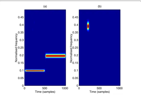
In a similar way to co-spectrum analysis, the real part of the cross-MST gives the in-phase components of the local spectra and the imaginary part of the cross-MST gives the in-quadrature components. Fig-ures 5a,b show the Co-MST and the Quadrature-MST amplitudes corresponding to the two signals x (t) and y(t), respectively. In the co-MST (Figure 5a), only the features that are in phase are present–those being the low and the medium frequency compo-nents. The higher frequency (which is out of phase) does not appear. In the quadrature-MST plot, only the out-of-phase components appear, which is the higher frequency component. As the example above was only for illustration, where the used signals have
0 500 1000
−2
−1 0 1 2
Time (samples)
Amplitude
(a)
Time (samples)
Nomalised frequency (Hz)
(c)
0 500 1000
0 0.1 0.2 0.3 0.4
0 500 1000
−2
−1 0 1 2
Time (samples)
Amplitude
(b)
Time (samples)
Nomalised frequency (Hz)
(d)
0 500 1000
0 0.1 0.2 0.3 0.4
straight and linear IF components and there is no noise; these results show that it is possible to study the coherence with sufficient high resolution using the cross-MST, whether for amplitude or phase cou-pling between two different spatially recorded com-ponents or signals.
5 Application to EEG seizure prediction
5.1 Phase synchrony information
The nonlinear interdependencies between fluctuations of brain physiological activities EEG-based recordings were intensively studied in pairs, and the synchrony flow differ-ences were compared [28]. It was shown in [29] that a neurological disorder in the brain can be detected by the random occurrence of its clinical manifestations, i.e., the seizure. There is also evidence that the nonseizure (inter-ictal) to seizure ((inter-ictal) transition is not an abrupt phenom-enon [29]. Hence, to provide a valuable insight into such mechanism, identification of early changes in EEG signals [28] can be used for prediction, prevention, and control of upcoming seizures. Different approaches have been employed for seizure prediction in the past. Some limited techniques based on visual inspection of the EEG signals or on linear methods have failed to detect specific and
sustained changes preceding seizures [28]. Other methods reported some changes based on the spectral contents [29], complexity [30], or spatio-temporal patterns of spikes [31]. Other recent approaches applied to newborn EEG-based seizure detection have been proposed such as time-frequency signal processing [32,33], and nonlinear signal processing [34,35].
Neuroscientists claim that when a focal seizure is gen-erated, synchronized brain activity is initially observed only in a small area of the brain; and, from this focus, the activity spreads spatially out to other brain areas in the temporal lobe over time [29]. Involving the seizure focus spread into its surrounding, a hyper-synchronous state happens and neighboring areas lose their synchro-nization with the other cortical regions around them [36]. In consequence, the seizure focus becomes isolated from the rest of the brain dynamics, making the consid-ered population of neurons inactive. Methods to track these changes using coherence and synchronization are being explored using EEG, for the purpose of predicting an impending seizure [36]. Phase synchronization was also shown to be a sensitive indicator of coupling between signals and as an important factor in the gen-esis of epileptic phenomenon [36]. Many studies suggest
Time (samples)
Normalised frequency (Hz)
0 200 400 600 800 1000
0 0.05 0.1 0.15 0.2 0.25 0.3 0.35 0.4 0.45
an underlying correlation between neuronal synchroni-zation and seizure development and onset [36,37]. Thus, the concept of phase synchrony helped to measure the synchrony evolution while the amplitude of the signals remained uncorrelated. In contrast with cross-correla-tion that measures linear relacross-correla-tionships only, a phase coupling approach is able to show the presence of non-linear coupling [38]. Moreover, phase synchrony can be used for non-periodic and for chaotic signals such as EEG [8,39]. Some authors used HT to measure phase synchrony between two signals [37,38,40]. However, the use of the HT assumes the signals have a narrow fre-quency band [1, p. 14], and it is not straightforward to extend the same analysis for broadband data. This assumption is usually seen to be ignored in the context of biomedical signals like the EEG [41]. As EEG signals are sometimes broadband (1-100 Hz) [41], the HT may not be able to correctly estimate the instantaneous phase of broadband signals. This raises the concern that the broadband phase synchronization analysis may lead to a misinterpretation of the results [41]. Therefore, when the signal is broadband it is necessary to pre-filter it in the frequency band of interest before applying the
HT, in order to get an better estimate of the phase [42]. Some authors used wavelet-based approach to analyze phase synchrony between pairs of EEG signals [13,43-45]. These time-varying measures of phase syn-chrony using wavelet or HTs are similar in their results. Both give a sharper phase synchrony estimates over time and frequency, especially at the low frequency range [46]. Although the wavelet and Hilbert based phase synchrony estimates address the issue of non-sta-tionarity of EEG signals, they suffer from limited time-scale resolution due to the limited number of available scales in the case of wavelets and the narrowband assumption in the case of HT. Moreover, the role of phase in wavelet analysis is not as well understood as it is for the Fourier transform, especially for orthonormal wavelet representations. Current complex wavelets such as Daubechies, dual tree, and Shannon wavelets do not have a direct relationship to the signal spectrum [18]. For these reasons, this article proposes to use the MST and the cross-MST to analyze the phase synchrony with the required resolution and with meaning, as the phase in the ST is meaningful and has the same concept as in the Fourier transform approach.
Normalised frequency
Time (samples) (a)
0 500 1000
0 0.05 0.1 0.15 0.2 0.25 0.3 0.35 0.4 0.45
Normalised frequency
Time (samples) (b)
0 500 1000
0 0.05 0.1 0.15 0.2 0.25 0.3 0.35 0.4 0.45
Figure 5co-MST and quadrature-MST.(a)The extracted in-phase components ofx(t) andy(t).(b)The extracted out-of-phase components of
5.2 Coherence analysis using cross-MST for simulated EEG seizure
Due to its non-stationarity characteristic, the newborn EEG seizure was modelled in the time-frequency domain [47-49]. using time-frequency characteristics previously identified in the newborn EEG seizure. Three models of newborn EEG seizure simulation were pre-viously proposed. One model is based on some physio-logical parameters of the brain and utilises a stationary sawtooth waveform [50]. This approach is extended in [47] to incorporate a single linear frequency modulation (LFM) signal. Another piecewise LFM model was defined for seizure based on non-stationary inputs to a nonlinear model [51]. We propose here a method of newborn EEG seizure analysis using the piecewise LFM pattern outlined in [47-50] to simulate the nonstationary behavior of the newborn EEG seizures.
The simulated signal is composed of several piecewise LFM components with different LFM slope parameters. Figure 6a represents three LFM piecewise signal with added Gaussian noise simulating the EEG seizure and the corresponding MST analysis. Figure 6b represents another three LFM piecewise signal with its MST, simi-lar to the one in Figure 5a except that the last compo-nent is out of phase compared to the two other components which are in phase in the two signals (More details are given in Appendix 2).
Key parts of the commented Matlab®code written to implement this method are given in Appendix 2.
Figure 7a represents the real part of the cross-MST of the two MSTs in Figure 6. We can see clearly that only the in-phase components are detected. However, in
Figure 7b, only the out-of-phase component is detected (the third component). Key parts of the commented Matlab® code written to implement this method are given in Appendix 1. Cross-MST of the Simulated EEG seizure showing the in-phase components (a) and the out-of-phase component (b).
5.3 Coherence Analysis using cross-MST for newborn EEG data
5.3.1 Background and analysis
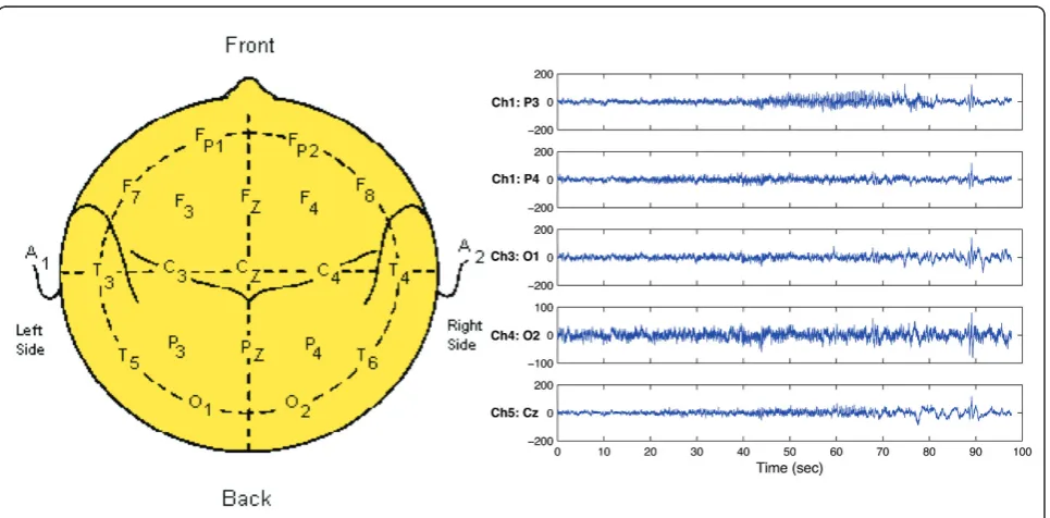
The data was acquired using a 20-channel Medelec Pro-file system (Medelec, Oxford Instruments, Old Woking, UK) at 256Hz sampling rate and marked by a pediatric neurologist from the Royal Children’s Hospital, Bris-bane, Australia. The experiment was conducted as part of a long term collaboration between Prof. Boashash, Director of the SPRC and Prof. Paul Colditz, Director of the Perinatal Research Centre at the University of Queensland. Measurements were made from a number of sick babies and this work was previously reported in [52]. Five monopolar channels (O1, O2, P3, P4, Cz) out of the 14 recorded signals according to the 10-20 stan-dard [53] modified for newborn subjects were selected from newborn EEG dataset. The data were analysed to investigate the coherence and phase coupling interhemi-spheric and intrahemiinterhemi-spheric interactions during an EEG seizure period. Figure 8a shows the 10-20 standard map of the 20-channel EEG recorder.
To study the phase coupling between the five chan-nels; we apply the MST to the five signals recorded from the five channels corresponding to P3, P4, O1, O2, and Cz, respectively. The location of the electrodes for
the five channels is shown in Figure 8a. Then, we apply the cross-MST function to analyze the in-phase and out-of-phase components in time-frequency space between the five channels. As mentioned previously, the real part of the cross-MST function gives the in-phase components of the local spectra; and the imaginary part of the cross-MST function gives the in-quadrature com-ponents. Figure 8 show the in-phase components for the connectivity between channels. From the all 25 possible connectivities shown, Figure 9 indicates that a strong phase synchrony exist in the last few seconds of the recording. This is shown by a peak in the real cross-MST images around 90s. This is in agreement with the
recorded signals shown in the time domain (see Figure 8b) as at the corresponding time (90 s) a peak with high amplitude is appearing in the signals. This may explain that at this time (around 90s) the pulses coming from different group of neurone are in phase and when they are added together, the sum results in high peak ampli-tude. This interpretation will not be possible if we just look at the signals amplitude from Figure 8b. The time signals recorded amplitude does not give a phase infor-mation to justify the synchrony; however, the cross-MST shows clearly this phase synchrony by a high peak amplitude in the real part present in the connectivity images (Figure 9).
Figure 7Cross-MST EEG. Cross-MST of the simulated EEG seizure showing the in-phase components(a)and the out-of-phase component(b).
Figure 10 represents the imaginary part of the cross-STs which reveal the out-phase behavior between the five channels. Note that there is no activity in the diago-nal images of Figure 10. This is because the diagodiago-nal represents the self-coherence between the five channels, hence there is no out-of-phase in this case; which is consistent as a signal can’t be out-of-phase with itself. From the off-diagonal images, we can see that most of the channels exhibit an out of phase behavior mostly in the period 40-80 s corresponding probably to the important duration of the appearance of the seizure. Some out-of-phase components are also present before this 40-80 s period in some channels, which can be explained by the fact that the seizure is not appearing in the same time and with the same way in the spatially different parts of the brain from where the EEG signals are recorded. The end of seizure can be explained by the disappearance of the out-of-phase components and the appearance of the out-of-phase components.
5.3.2 Results, discussion and interpretation
The results on the real newborn EEG data show that the cross-ST can be used as a effective tool to study the phase coupling between channels. These results suggest that during the seizure period, all the components lose synchrony and are out of phase. This can be seen like a disorder in the neuronal activity during the seizure
interval. This observed irregularity in the time-frequency patterns during the seizure period (40-80 s) between two hemispheres in the posterior area suggest that dif-ferent regions and not only one specific region may be causing the seizure. In contrast, the components (neural activity) became synchronized again after the seizure activity vanishes. This EEG seizure application demon-strates that the time-frequency coherence is an appro-priate tool to study the phase coupling between different signals recorded from different spatially sepa-rated electrodes. This study is performed by the cross-MST which has a referenced phase at the origin, a prop-erty that allows the study of phase coupling and time-frequency coherence between the neuronal activities. Although the cross-MST represent a good candidate tool to analyze such coupling behavior, this methodol-ogy can be extended to other cross-time-frequency methods with high time-frequency resolution such as the QTFDs. In particular, the time-frequency coherence using the cross-WVD has a useful property for cross spectral analysis, and can be interpreted as a time and frequency dependent correlation coefficients [26].
6 Conclusions and perspectives
This article applies the concept of time-frequency coherence using the cross-MST which is a
time-Ch1−−−>Ch1
0 0.2 0.4
0 20 40 60 80
Ch1−−−>Ch2
0 0.2 0.4
0 20 40 60 80
Ch1−−−>Ch3
0 0.2 0.4
0 20 40 60 80
Ch1−−−>Ch4
0 0.2 0.4
0 20 40 60 80
Ch1−−−>Ch5
0 0.2 0.4
0 20 40 60 80
Ch2−−−>Ch1
0 0.2 0.4
0 20 40 60 80
Ch2−Ch2
0 0.2 0.4
0 20 40 60 80
Ch2−−−>Ch3
0 0.2 0.4
0 20 40 60 80
Ch2−−−>Ch4
0 0.2 0.4
0 20 40 60 80
Ch2−−−>Ch5
0 0.2 0.4
0 20 40 60 80 Time (sec)
Ch3−−−>Ch1
0 0.2 0.4
0 20 40 60 80
Ch3−−−>Ch2
0 0.2 0.4
0 20 40 60 80
Ch3−−−>Ch3
0 0.2 0.4
0 20 40 60 80
Ch3−−−>Ch4
0 0.2 0.4
0 20 40 60 80
Ch3−−−>Ch5
0 0.2 0.4
0 20 40 60 80
Ch4−−−>Ch1
0 0.2 0.4
0 20 40 60 80
Ch4−−−>Ch2
0 0.2 0.4
0 20 40 60 80
Ch4−−−>Ch3
0 0.2 0.4
0 20 40 60 80
Ch4−−−>Ch4
0 0.2 0.4
0 20 40 60 80
Ch4−−−>Ch5
0 0.2 0.4
0 20 40 60 80
Ch5−−−>Ch1
0 0.2 0.4
0 20 40 60 80
Ch5−−−>Ch2
0 0.2 0.4
0 20 40 60 80
Normalised Frequency (Hz) Ch5−−−>Ch3
0 0.2 0.4
0 20 40 60 80
Ch5−−−>Ch4
0 0.2 0.4
0 20 40 60 80
Ch5−−−>Ch5
0 0.2 0.4
0 20 40 60 80
varying cross-spectral analysis method obtained by extending the S-transform. The article demonstrates the ability of this time-frequency coherence using the cross-MST to study the functional neuronal phase syn-chrony between channels. The performance of the phase synchrony estimation using the cross-MST are evaluated both by simulated EEG seizure using a piece-wise LFM signal to extract the in and out-of-phase components, and through the analysis of seizure EEG abnormalities in the newborn, where the dynamics of brain changes rapidly and the neurones lose their syn-chrony during seizure. Both the simulated and new-born results show cross-MST phase and synchrony estimation to be more robust to noise. The resolution obtained by the MST shows almost twofold improve-ment over the standard ST approach. Future work will concentrate on a comparison study between the pro-posed method and other existing time-frequency tech-niques such as Wigner-Ville and QTFDs based methods, for both simulated and real EEG data to develop more efficient time-varying phase and syn-chrony estimation for nonstationary signals, and such
results will appear elsewhere. The proposed method can be extended to other physiological problems where the phase coupling is relevant, such in cardio-respira-tory relationship, for example, where the coupling can be affected by cardio-vascular diseases.
Acknowledgements
The Authors wish to thank Prof Paul Colditz, Director of the Perinatal Research Centre, and his team for pro-viding the real newborn EEG data presented in this paper. The second author acknowledges funding by QNRF, Qatar Foundation under grant NPRP 09 465 2 174. The first author also acknowledges Weatherford for giving permission to publish this work.
Appendix
1 Computing the MST % Compute the MST
[M,N]=size(sig); % get the
length of the signal N2=fix(N/2); j = 1; if N2*2==N; j = 0;end Ch1−−−>Ch1
0 0.2 0.4
0 20 40 60 80 Ch1−−−>Ch2
0 0.2 0.4
0 20 40 60 80 Ch2−−−>Ch3
0 0.2 0.4
0 20 40 60 80 Ch1−−−>Ch4
0 0.2 0.4
0 20 40 60 80 Ch1−−−>Ch5
0 0.2 0.4
0 20 40 60 80 Ch2−−−>Ch1
0 0.2 0.4
0 20 40 60 80 Ch2−−−>Ch2
0 0.2 0.4
0 20 40 60 80 Ch2−−−>Ch3
0 0.2 0.4
0 20 40 60 80 Ch2−−−>Ch4
0 0.2 0.4
0 20 40 60 80 Ch2−−−>Ch5
0 0.2 0.4
0 20 40 60 80 Time (sec) Ch3−−−>Ch1
0 0.2 0.4
0 20 40 60 80 Ch3−−−>Ch2
0 0.2 0.4
0 20 40 60 80 Ch3−−−>Ch3
0 0.2 0.4
0 20 40 60 80 Ch3−−−>Ch4
0 0.2 0.4
0 20 40 60 80 Ch3−−−>Ch5
0 0.2 0.4
0 20 40 60 80 Ch4−−−>Ch1
0 0.2 0.4
0 20 40 60 80 Ch4−−−>ch2
0 0.2 0.4
0 20 40 60 80 Ch4−−−>Ch3
0 0.2 0.4
0 20 40 60 80 Ch4−−−>Ch4
0 0.2 0.4
0 20 40 60 80 Ch4−−−>Ch5
0 0.2 0.4
0 20 40 60 80 Ch5−−−>Ch1
0 0.2 0.4
0 20 40 60 80 Ch5−−−>Ch2
0 0.2 0.4
0 20 40 60 80
Normalised Frequency (Hz) Ch5−−−>Ch3
0 0.2 0.4
0 20 40 60 80 Ch5−−−>Ch4
0 0.2 0.4
0 20 40 60 80 Ch5−−−>Ch5
0 0.2 0.4
0 20 40 60 80
f=[0:N2 -N2+1-j:-1]/N; %frequency
MST=zeros(N2+1,N); %allocate
mem-ory for positive frequencies of MST.
SIG=fft(sig,N); %compute the
sig-nal spectrum
g=(1/N)*f+4*var(sig); %parameter
gamma
for i = 2:N2
SIGs=circshift(SIG,[0,-(i-1)]); %
circshift the spectrum SIG
W=(g(i)/f(i))*2*pi*f; %
Scale Gaussian
G=exp((-W.^2)/2); %W in
Fourier domain
MST(i,:)=ifft(SIGs.*G);
%Com-pute the complex values of MST end
imagesc(abs(MST)’);
set(gca,’Ydir’,’Normal’); %default Y
axis in imagesc is inverted. 2 Generation of piece-wise LFM
%Piecewise LFM chirp generation for EEG Seizure simulation
fs = 50; %Sampling frequency
t1=(-5:1/50:5); t2=(-2.5:1/50:2.5); t3= (-5:1/50:5); % time for the first,
% the second and the % third segment
t=[t1 t2 t3]; % total time
for the Piecewise LFM.
f00 = 2.626; f01 = 1.83; f10 = 1.751; %
start frequencies
a1=-0.7; a2=-0.6; a3 = 0.2; % chirp
rates or slope
ph1 = 2*pi*f00*t1+0.5*a1*t1.*t1; %
quadratic phase of piecewise LFM1
ph2 = 2*pi*f01*t2+0.5*a2*t2.*t2; %
quadratic phase of piecewise LFM2
ph3 = 2*pi*f10*t3+0.5*a3*t3.*t3; %
quadratic phase of piecewise LFM3
lfm1=exp(1i*ph1);lfm2=exp(1i*ph2);
lfm3=exp(1i*ph3); %generate piecewise
LFMs
lfm=[real(lfm1) real(lfm2) imag(lfm3)]; % put all in one signal LFM.
sig=lfm+0.2*randn(length(lfm),1)’; %
add gaussian noise 3 Computing the cross-MST
%The cross-MST, co-MST and quadrature-MST
%Computing the Cross-MST of two signal x (t) and y(t)
%having as modified ST: MST1 and MST2, respectively.
% 1.Compute MST1 and MST2 using the related code in appendix A.
% 2.Compute the cross-MST between MST1 and MST2
cross MST = MST1.*conj(MST2); %Get the cross-MST.
% 3. Get the out-of-phase components
imagesc(imag(cross_MST)); set
(gca,’Ydir’,’Normal’)
% 4. Get the in-phase components
imagesc(real(cross_MST)); set
(gca,’Ydir’,’Normal’)
Author details
1
Weatherford, East Leake, Leicestershire LE12 6JX, UK2Perinatal Research Centre and UQ Centre for Clinical Research, Royal Brisbane and Women’s Hospital, The University of Queensland, Hertson QLD 4029, Australia3College of Engineering, Qatar University, Doha, Qatar
Competing interests
The authors declare that they have no competing interests.
Received: 3 October 2011 Accepted: 28 February 2012 Published: 28 February 2012
References
1. B Boashash,Time Frequency Signal Analysis and Processing: A Comprehensive Reference(Elsevier, Oxford, 2003)
2. J Imberger, B Boashash, Application of the Wigner-Ville distribution to temperature gradient microstructure: a new technique to study small-scale variations. Phys Oceanograp.16(12), 1997–2012 (1986). doi:10.1175/1520-0485(1986)0162.0.CO;2
3. B Boashash, Note on the use of the Wigner-Ville distribution for time-frequency signal analysis. IEEE Trans Acoust Speech Signal Process.36(9), 1518–1521 (1988). doi:10.1109/29.90380
4. W-k Lu, Q Zhang, Deconvolutive short-time fourier transform spectrogram. IEEE Signal Process Lett.16(7), 576–579 (2009)
5. Y Zhao, LE Atlas, RJ Marks, The use of cone-shape kernels for generalized time-frequency representations of nonstationary signals. IEEE Trans Acoust Speech Signal Process.38(7), 1084–1091 (1990). doi:10.1109/29.57537 6. H Choi, WJ Williams, Improved time-frequency representation of
multicomponent signals using exponential kernels. IEEE Trans Acoust Speech Signal Process.37(6), 862–871 (1989). doi:10.1109/ASSP.1989.28057 7. RG Stockwell, L L Mansinha, RP Lowe, Localisation of the complex
spectrum: theStransform. IEEE Trans Signal Process.44(4), 998–1001 (1996). doi:10.1109/78.492555
8. M Rosenblum, A Pikovsky, J Kurths, Phase synchronization of chaotic oscillators. Phys Rev Lett.76(11), 1804–1807 (1996). doi:10.1103/ PhysRevLett.76.1804
9. WA Gardner,Introduction to Random Processes: with Applications to Signals and Systems(McGraw-Hill Inc., US, 1990)
10. LH Koopmans, inThe Spectral Analysis of Time Series; in Probability and Mathematical Statistics, vol. 22. (Academic Press, London, UK, 1995) 11. JS Bendat, AG Piersol,Random Data Analysis and Measurement Procedures
(Wiley, New York, 2000)
12. B Boashash, Estimating and interpreting the instantaneous frequency of a signal. I. Fundamentals. IEEE, Proceedings.80(4), 520–538 (1992). doi:10.1109/5.135376
13. D Li, R Jung, Quantifying coevolution of nonstationary biomedical signals using time-varying phase spectra. Ann Biomed Eng.28(9), 1101–1115 (2000) 14. K Gochenig,Foundations of Time-Frequency Analysis(Birkhauser, Boston,
2001)
16. W Lin, M Xiaofeng, An adaptative generalizedS-transform for instantaneous frequency estimation. Signal Process.91(8), 1876–1886 (2011). doi:10.1016/j. sigpro.2011.02.010
17. E Sejdic, L Stancovic, M Dakovic, J Jiang, Instantaneous frequency estimation using theS-transform. IEEE Trans Signal Process Lett.15, 309–312 (2008)
18. RG Stockwel, inWhy use the S-transform, vol. 52, ed. by A Wong (Fields Institute Communications, Providence, 2007), pp. 279–309. Pseudo-Differential Operators: PDEs and Time-Frequency Analysis 19. B Boashash, PJ O’Shea, Use of the cross Wigner-Ville distribution for
estimation of instantaneous frequency. IEEE Trans Signal Process.41(3), 1439–1445 (1993). doi:10.1109/78.205752
20. L Mansinha, RG Stockwell, RP Lowe, Pattern analysis with two-dimensional spectral localisation: applications of two dimensionalS-transforms. Phys A.
239, 286–295 (1997). doi:10.1016/S0378-4371(96)00487-6
21. PD McFadden, JG Cook, LM Forster, Decomposition of gear vibration signals by the generalized S transform. Mechan Syst Signal Process.13, 691–707 (1999). doi:10.1006/mssp.1999.1233
22. CR Pinnegar, L Mansinha, TheS-transform with windows of arbitrary and varying shape. Geophysics.68, 381–385 (2003). doi:10.1190/1.1543223 23. G Kondaveeti, MJB Reddy, DK Mohanta, Power quality analysis on EHV
transmission line using modifiedS-transform, in9th International Conference on Environment and Electrical Engineering (EEEIC2010), Prague, Czech Republic, IEEE-PES, pp. 337–340 (16-19 May 2010)
24. GV Nithin, SS Sitanshu, L Mansinha, KF Tiampo, G Panda, Time localised band filtering using modifiedS-transform, inProceedings of the International Conference on Signal Processing Systems (ICSPS09), Singapore, pp. 42–46 (15-17 May 2009)
25. W Czaja, G Kutyniok, D Speegle, The geometry of sets of parameters of wave packet frames. Appl Comput Harmon Anal.20, 108–112 (2006). doi:10.1016/j.acha.2005.04.002
26. LB White, B Boashash, Cross spectral analysis of nonstationary processes. IEEE Trans Inf Theory.36(4), 830–835 (1990). doi:10.1109/18.53742 27. P Boles, B Boashash, The cross Wigner-Ville distribution–a two dimensional
analysis method for the processing of vibroseis seismic signals, inProc International Conference on Acoustics, Speech, and Signal Processing (ICASSP), IEEE-ICASSP, NY, USA, pp. 904–907 (11-14 Apr 1988)
28. M Chavez, MLV Quyen, V Navarro, M Baulac, J Martinerie, Spatio-temporal dynamics prior to neocortical seizures: amplitude versus phase couplings. IEEE Trans Biomed Eng.50(5), 571–583 (2003). doi:10.1109/
TBME.2003.810696
29. MD Alessandro, R Esteller, G Vachtsevanos, A Hinson, J Echauz, B Litt, Epileptic seizure prediction using hybrid feature selection over multiple intracranial EEG electrode contacts: a report of four patients. IEEE Trans Biomed Eng.50(5), 603–615 (2003). doi:10.1109/TBME.2003.810706 30. RG Andrzejak, F Mormann, G Widman, T Kreuz, CE Elger, K Lehnertz,
Improved spatial characterization of the epileptic brain by focusing on nonlinearity. Epilepsy Res.69(2), 30–44 (2006)
31. D Gupta, CJ James, WP Gray, Phase synchronization with ica for epileptic seizure onset detection in the long term EEG, inProc 4th IET Int Conf on Intelligent, Advanced in Medicine, Signal and Information Processing (MEDSIP), IET 2008, Seattle, USA, pp. 1–4 (21-22 July 2008)
32. H Hassanpour, M Mesbah, B Boashash, Timefrequency based newborn EEG seizure detection using low and high frequency signatures. Physiol Meas.
25, 935–944 (2004). doi:10.1088/0967-3334/25/4/012
33. M Rankine, LV Mesbah, B Boashash, Automatic newborn EEG seizure spike and event detection using adaptive windowoptimization, inProc ISSPA 2005, IEEE 2005, Sydney, Australia, pp. 187–190 (Aug 2005)
34. M Roessgen, AM Zoubir, B Boashash, Seizure detection of newborn eeg using a model-based approach. IEEE Trans Biomed Eng.45(6), 673–685 (1998). doi:10.1109/10.678601
35. J Altenburg, R Vermeulen, R Strijers, W Fetter, C Stam, Seizure detection in the neonatal EEG with synchronization likelihood Clin Neurophysiol.114, 50–55 (2003)
36. MLV Quyan, Anticipating epileptic seizures: from mathematics to clinical applications. C R Biol.328(2), 187–198 (2005). doi:10.1016/j.crvi.2004.10.014 37. TI Netoff, SJ Schiff, Decreased neuronal synchronization during experimental
seizures. J Neurosci.22(16), 7297–7307 (2002)
38. M Rosenblum, A Pikovsky, J Kurths, C Schafer, PA Tass, Phase synchronization: from theory to data analysis, inNeuro-Informatics and
Neural Modeling, ed. by F Moss, S Gielen (Elsevier, North-Holland, 2001), pp. 279–321
39. F Mormann, K Lehnertz, P David, CE Elger, Mean phase coherence as a measure for phase synchronization and its application to the EEG of epilepsy patients. Phys D Nonlinear Phen.144(3-4), 358–369 (2000). doi:10.1016/S0167-2789(00)00087-7
40. W De-Clercq, P Lemmerling, W Van-Paesschen, S Van-Huffel,
Characterization of in-terictal and ictal scalp EEG signals with the Hilbert transform, inProc 25th Annu International Conf of the IEEE-EMBS, Cancun, Mexico, pp. 2459–2462 (17-21 Sept 2003)
41. D Gupta, CJ James, Narrowband vs. broadband phase synchronization analysis applied to independent components of ictal and interictal EEG, in
Proceedings of the 29th Annual International Conference of the IEEE-EMBS, ed. by Y Smith (Lyon, France, 2007), pp. 3864–3867
42. L Angelini, LMD Tommaso, M Guido, Hu PC, K Ivanov, D Marinazzo, G Nardulli, L Nitti, M Pellicoro, C Pierro, S Stramaglia, Steady-state visual evoked potentials and phase synchronization in migraine patients. Phys Rev Lett.93(3), 38103–38106 (2004)
43. H Adeli, Z Zhou, N Dadmehr, Analysis of EEG records in an epiliptic patient using wavelet transform. Neurosci Methods.123, 69–87 (2003). doi:10.1016/ S0165-0270(02)00340-0
44. P Bob, M Susta, K Glaslova, EEG phase synchronization in patients with paranoid schizophrenia. Neurosci Lett.447, 73–77 (2008). doi:10.1016/j. neulet.2008.09.055
45. JP Lachaux, A Lutz, D Rudrauf, D Cosmelli, M Le-Van-Quyen, J Martinerie, F Varela, Estimating the time course of coherence between single-trial brain signals: an introduction to wavelet coherence. Neurophysiol Clin.32(1-3), 1–18 (2002)
46. MLV Quyan, J Foucher, E Lachaux, JP Rodriguez, A Lutz, J Martinerie, FJ Varela, Comaprison of Hilbert transform and wavelet methods for the analysis of neural synchrony. Neurosci Methods.111(2), 83–98 (2001). doi:10.1016/S0165-0270(01)00372-7
47. B Boashash, M Mesbah, Time-frequency methodology for newborn electroencephalo-graphic seizure detection, inApplications in Time-frequency Signal Processing, ed. by A Papandreou-Suppappola (CRC Press LLC, Boca Raton, 2002), pp. 339–369
48. B Boashash, M Mesbah, Time-frequency approach for newborn EEG seizure detection. IEEE Eng Med Biol Mag.20(5), 54–64 (2001)
49. B Boashash, M Mesbah, P Colditz, Newborn EEG seizure pattern characterisation using time-frequency analysis, inProc International Conference on Acoustics, Speech, and Signal Processing (ICASSP), IEEE-ICASSP 2001, Salt Lake City, USA, pp. 1041–1044 (7-11 May 2001)
50. M Roessgen, A Zoubir, B Boashash, Seizure detection of newborn EEG using a model based approach. IEEE Trans Biomed Eng.45(6), 673–685 (1998). doi:10.1109/10.678601
51. NJ Stevenson, M Mesbah, GB Boylan, PB Colditz, B Boashash, A nonlinear model of newborn EEG with nonstationary inputs. Ann Biomed Eng.38(9), 3010–3021 (2010). doi:10.1007/s10439-010-0041-3
52. P Celka, B Boashash, P Colditz, Pre-processing and time-frequency analysis of newborn EEG seizures. IEEE Eng Med Biol Mag.20(5), 30–38 (2001). doi:10.1109/51.956817
53. E Niedermeyer, F Lopes-da Silva,Electroencephalography: Basic Principles, Clinical Applications and Related Fields(Lippincott williams & Wilkins, Philadelphia, 2004)
doi:10.1186/1687-6180-2012-49