Resource Optimization for Networked Estimator with Guaranteed Estimation Quality

Guaranteed Estimation Quality

Thesis by Ling Shi

In Partial Fulfillment of the Requirements for the Degree of

Doctor of Philosophy

California Institute of Technology Pasadena, California

2009

Acknowledgements

Five years ago, I came to Pasadena for the first time, and everything was new and exciting to me. Now I am about to leave for a new stage of life. The past five years has been one of the best times in my life, and I truly enjoyed every single day I spent here, not just for the great facilities, but more importantly for the many great people I have met and worked with.

My most sincere thanks and gratitude go to my advisor, Prof. Richard Murray. I remember how he motivated and taught me to do research from the very beginning and encouraged me on my first paper at Caltech. He has always been a source of inspiration and a source of instant help. Thank you for all your support over the past few years, for which I am truly and always grateful.

Prof. Karl H. Johansson is a great mentor. I enjoyed very much the collaboration with him when he spent his sabbatical here two years ago. The series of work that I did with him during that time lay out the foundation of my thesis. Thank you for your guidance, support, and for your kind hosting of my visit in Nov. 2007.

The conversation with Prof. John Doyle in summer 2006 inspired me to look at multi-sensors instead of single-sensor networked control applications, and focus on the interaction between network topology and estimator and controller design.

Prof. Mani Chandy and Prof. Joel Burdick are kindly willing to serve as my thesis committee members beside Prof. Richard Murray, Prof. Karl H. Johansson, and Prof. John Doyle. I would like to thank you all for your precious time.

My former advisors, Prof. Zexiang Li and Li Qiu at the Hong Kong University of Science and Technology continue to encourage and support me even after I graduated in 2002. I would like to thank them for their time and help over these years. Prof. John Koo is a great friend, and I would like to thank him for his support and help over the years too.

It has been my great pleasure to spend the previous five years with the CDS family, especially with the Murray group, who make me feel I am at home. I very much enjoyed the weekly meetings with Michael Epstein, my most frequent collaborator in the first few years, whose encouragement and proficient computer skills often made our work very easy. Michael is also a great friend, and he is always ready to offer his help whenever needed; “Ma Shang, Ma Shang,” he says. The collaboration with Ahbishek Tiwari at my second year opened the door to a series of work on networked control systems. I spent the first year with Dennice Gayme, Shaunak Sen, and Dmitriy Kogan taking the same set of courses. I got a lot of help from Xin Liu, Lun Li, Zhipu Jin, Jiantao Wang, Lijun Chen, and Dr. Wang Sang Koon during my first few years at CDS and Caltech. For all other CDS family members: I would like to thank you all and you have made my stay at Caltech so enjoyable. I am grateful for the Chinese community here. In particular, I would like to thank all Braun residents: Kevin Ko, Xiaojie Gao, Changlin Pang, Chengzhong Zhang, Xin Guo, Zhaoyan Zhu, and Hao Jiang. I enjoyed my first two years here staying with them.

I would like to thank a few friends: Guanfeng Liu, Jijie Xu, Jian Cao, Yu Chen (for all your encouragement and support), Agostino Capponi (I enjoyed the collaboration with you), Nawaf Bou-Rabee (I enjoyed working with you for CDS 202), Stephen Backer (I enjoyed the apple pie that you prepared), Alex Backer (I enjoyed working with you as my intern), Jing Liu and Wei Liang (I enjoyed the delicious food prepared by your parents), Chunhui Gu (I enjoyed the many conversations with you), and Wen Yang (I enjoyed the many meals and conversations with you).

Tsuji at the career center, and Alice M. Sogomonian at the health center, who made my stay at Caltech particularly easy.

I enjoyed the Bible study every Saturday at the Brother House. I would like to thank Peter Tsui, Andy Pearce, Zhongtian Lin, Jing Wu, and their families, Zhuo Li, Zhaoyu Zhang, and other brothers and sisters. Thank you all for making my life so wonderful and happy.

Last but not least, I would like to thank my parents, my sister and her family, and my wife and her family for their strong support.

Abstract

Contents

Acknowledgements iii

Abstract vi

1 Introduction 1

1.1 Background . . . 1

1.2 Related Work . . . 3

1.3 Summary of Contributions and Overview of Thesis . . . 5

2 Preliminaries and Definitions 8 2.1 Definitions . . . 8

2.2 Kalman Filter and Modified Kalman Filter . . . 9

2.3 Math Preliminaries . . . 13

3 Kalman Filtering over Multihop Sensor Trees 16 3.1 Introduction . . . 16

3.2 Problem Set-up . . . 17

3.3 Optimal Estimation Over a Sensor Tree . . . 19

3.4 Example . . . 21

3.5 Some Useful Inequalities . . . 23

4 Minimizing Sensor Energy 26 4.1 Introduction . . . 26

4.2 Problem Set-up . . . 27

4.3 Minimizing Sensor Energy . . . 29

5.4 Examples . . . 50

6 Minimizing Buffer Length 56 6.1 Introduction . . . 56

6.2 Problem Setup . . . 57

6.3 Sensor without Computation Capability . . . 59

6.4 Sensor with Computation Capability . . . 69

6.5 Examples . . . 73

7 Conclusions and Future Work 78 7.1 Concluding Remarks . . . 78

7.2 Future Directions . . . 79

Chapter 1

Introduction

1.1

Background

Advances in fabrication, modern sensor and communication technologies, and computer architecture have enabled a variety of new networked sensing and control applications. In many of these applications, there is an economic incentive towards using off-the-shelf sensors and standardized communication solutions. A consequence of this is that the individual hardware components might be of relatively low quality and that communication resources are quite limited.

Networked sensing and control applications are found in a growing number of areas, including automobiles, autonomous vehicles, environmental monitoring, industrial automa-tion, power distribuautoma-tion, space exploraautoma-tion, surveillance, and transportation. For example, Alice is an autonomous vehicle that was developed at California Institute of Technology for the 2005 DARPA Grand Challenge [11]. The sensors mounted on Alice include an iner-tial measurement unit (IMU), global positioning system (GPS), velocity and measurement range sensors, and stereo vision. To allow the vehicle to autonomously navigate through its environment, sensor data are fused to provide Alice an estimate of its own state and of the environment around it. The heterogeneous set of sensors is connected with the computation platform through an Ethernet local area network providing an architecture for networked estimation and control.

temperature, humidity, pressure, air density, etc. Depending on the routing protocol as well as the available resources (network bandwidth, node energy, etc.), the collected data are transmitted to their final destination, usually a fusion center, at appropriate times. For example, the Pursuer-Evader game (Figure 1.1) carried out at UC Berkeley [47] consists of hundreds of tiny sensor nodes which are capable of measuring the state of incoming evaders. The measured information is sent back to a computational unit via multi-hop communica-tion paths, and corresponding control laws are computed and sent to the pursuers.

Figure 1.1: Pursuer Evader Game. Photo Courtesy: UC Berkeley

filter. The Kalman filter [24] is a well-established methodology for model-based fusion of sensor data [2, 15, 16, 23] that has played a central role in systems theory and has found wide applications in many fields such as control, signal processing, and communications. In the standard Kalman filter, it is assumed that sensor data are transmitted along perfect communication channels and are available to the estimator instantaneously, and no interac-tion between communicainterac-tion and control is considered. This underlying assumpinterac-tion breaks when networks, especially wireless networks, are used in sensing and control systems for transmitting data from sensors to controller and/or from controller to actuator.

Many difficulties are inherent in these networked sensing and control systems, for exam-ple, constrained communication and computation capabilities, and limited energy resources, which are frequently seen in a wireless sensor network [13]. Communication between net-work nodes is limited, particularly, if nodes are located physically far way from each other. It takes time to transfer information from one node to another. As a consequence, the net-works typically induce many new issues such as limited bandwidth, packet loss, and delay. These constraints affect system performance or even stability, and cannot be neglected when designing estimation and control algorithms; this has inspired a lot of research in control with communication constraints.

The rapid developments of networked sensing and control technologies enable drastic change of the architecture and embedded intelligence in these systems. The theory and design tools for these systems are not fully developed, but there is a lot of current research, some of which is described next.

1.2

Related Work

are given in [20,55]. The drawback of using mean covariance matrix as a stability measure is that it may conceal the fact that events with arbitrarily low probability may make the mean value diverge. Different from [20, 45, 55], the stability of the Kalman filter was investigated via a probabilistic approach in [41].

One way to deal with the problem of asynchronous generation of sensor data is to use event-triggered control instead of conventional time-triggered control [3, 25]. How to effi-ciently encode control information for event-triggered control over communication channels with severe bandwidth limitations was discussed in [4]. A scheme based on multi-description coding for lossy networks, but limited to the estimation, was considered by Jin et al. [21]. A compensation scheme in the controller for the variations on the transport layer that such routing protocols give rise to was presented by Witrant et al. [52]. A robust control approach to control over multi-hop networks was discussed in [37].

Kalman filtering under certain information constraints, such as decentralized implemen-tation, has been extensively studied [44]. Implementations for which the computations are distributed among network nodes were considered by Alriksson and Rantzer [1]. The in-teraction between Kalman filtering and how data is routed on a network seems to be less studied. Routing of data packets in networks is typically done based on the distance to the receiver node [5]. Some recent work addresses how to couple data routing with the sensing task using information theoretic measures [22]. A heuristic algorithm for event detection and actuator coordination was proposed by Ngai et al. [35]. For control over wireless sensor networks, the experienced delays and packet losses are important parameters. Random-ized routing protocols that give probabilistic guarantees on delay and loss were proposed in [6, 27].

time-stamped and thus transmission delays are known to the filter, the delays in networked systems are random in nature. Thus, the state augmentation and the reorganized innovation approaches are generally not applicable.

For the problem of randomly delayed measurements, Ray et al. [39] presented a modifi-cation of the conventional minimum variance state estimator to accommodate the effects of the random arrival of measurements, whereas a suboptimal filter in the least-mean-square sense is given in [57]. In [30], a recursive minimum variance state estimator was presented for linear discrete-time partially observed systems where the observations are transmitted by communication channels with randomly independent delays. Using covariance information, recursive least-squares linear estimators for signals with random delays were studied in [34]. Furthermore, the filtering problems with random delays and missing measurements have been investigated in [40, 48, 51] via the linear matrix inequality and the Riccati equation approaches, respectively.

More related work can be found in a recent survey of networked control systems in [17].

1.3

Summary of Contributions and Overview of Thesis

The main contribution of this thesis work is to tackle the aforementioned networked con-trol problems by optimizing the limited resources of those networks while guaranteeing a certain level of desired estimation quality. In particular, I consider minimizing the sensor energy usage, maximizing the network lifetime, and minimizing the buffer length, with each corresponding to a class of networked sensing and control applications. The scenarios and algorithms investigated are:

• (Chapter 3) Optimal estimation algorithm over a sensor tree is presented with a closed-form expression on the steady-state error covariance.

• (Chapter 4) A sensor tree reconfiguration algorithm is presented to minimize the sensor energy usage.

• (Chapter 5)A sensor tree construction and scheduling algorithm is presented to max-imize the sensor network lifetime.

are represented by a tree in Chapter 3.

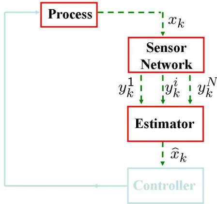
Figure 1.2: State Estimation over a Wireless Sensor Network

We further consider the network lifetime maximization problem in Chapter 5, where we first motivate that by minimizing the overall energy cost is not sufficient to maximize the network lifetime. Therefore we propose a sensor tree construction and scheduling algorithm that maximizes the network lifetime.

Figure 1.3: State Estimation over a Packet Delaying Network

In Chapter 6, we study the performance of a Kalman filter under random measurement delay (Figure 1.3). The probability distribution of the delay is assumed to be given and we give a complete characterization of filter performance via a probabilistic approach. Due to the limited computation capability of the filtering center and also in consideration of the fact that a late-arriving measurement related to the system state in the far past may not contribute much to the improvement of the accuracy of the current estimate, it is practi-cally important to determine a proper buffer length for measurement data within which a measurement will be used to update the current state and beyond which the data will be discarded. The buffer provides a tradeoff between the filter performance and computational load. In this thesis, for a given buffer length, we give lower and upper bounds for the prob-ability at which the filtering error covariance is within a prescribed bound, i.e.,Pr[Pk ≤M]

for some given M. The upper and lower bounds can be easily evaluated by the probabil-ity distribution of the delay and the system dynamics. An approach for determining the minimum buffer length for a required performance in probability is given and an evaluation on the number of expected filter updates is provided. Both the cases of sensor with and without computation capability for filter updates are considered.

Chapter 2

Preliminaries and Definitions

In this chapter, some definitions are provided which are used frequently in remaining chap-ters. A brief introduction to the Kalman filter and the modified Kalman filter is also included, upon which the main results of later chapters rely.

2.1

Definitions

The following definitions are frequently used throughout later chapters. Z+ _{denotes the set}

of nonnegative integers. IRn is the realn-dimensional vector space. IRn×n is the set ofnby n real matrices. Sn

+ is the set of nby n positive semidefinite matrices. When X ∈Sn+, we

simply writeX _≥0; whenX is positive definite, we write X >0.

We are frequently dealing with systems with parameters (A, C, Q, R), whereA_∈IRn×n and C _∈ IRm×m are the system and sensor measurement matrices, Q _∈ Sn

+ and R ∈ Sm+

with R > 0 are the process and measurement noise covariance matrices respectively, e.g., in Eqn (2.7) and (2.8). We define the functionh_[A,Q]:Sn+ →Sn+ as

h_[A,Q](X),AXA

′

+Q. (2.1)

As we shall see shortly, applyingh to the previous error covariance matrix corresponds to the time update of the standard Kalman filter. Similarly, we define the functiong_[A,C,Q,R]:

Sn

+→Sn+ as

and the function ˜g_[C,R]:Sn

+→Sn+ as

˜

g_[C,R](X),X−XC

′

[CXC′+R]−1CX. (2.3)

Theng and ˜g correspond to the measurement update for the a priori and a posteriori error covariance matrices respectively in the standard Kalman filter. We simply writeh_[A,Q]ash, g_[A,C,Q,R] asg orgC, and ˜g[A,C,Q,R]as ˜g or ˜gC when there is no confusion on the underlying

parameters [A, C, Q, R]. It is easy to see that

g=h_◦g.˜ (2.4)

We denote λi(A) as the i-th eigenvalue ofA and ρ(A) as spectral radius ofA, i.e.,ρ(A) =

maxi|λi(A)|. We say A is stable if ρ(A) < 1, and A is unstable if A is not stable. For

functions f, f₁, f₂ :Sn

+→Sn+,f1◦f2 is defined as

f1◦f2(X),f1 f2(X), (2.5)

and ftis defined as

ft(X) ,f_◦f_{◦ · · · ◦}f

| {z }

t times

(X). (2.6)

For a random variable X, we write its expectation value asE[X] and its conditional prob-ability given another random variableY asPr[X_|Y].

2.2

Kalman Filter and Modified Kalman Filter

Kalman Filter Preliminaries

Consider the following linear discrete time system:

xk = Axk−₁+wk−₁, (2.7)

yk = Ckxk+vk. (2.8)

In the above equations, xk ∈ IRn is the state vector, yk ∈ IRm is the observation vector,

Assume a linear estimator receives yk and computes the optimal state estimate at each

timek. Define the following terms at the estimator:

ˆ

x−_{k ,} E[xk|all measurements up tok−1],

ˆ

xk , E[xk|all measurements up tok],

P_k− _, E[(xk−xˆ

−

k)(xk−xˆ

−

k)

′ ], Pk , E[(xk−xˆk)(xk−xˆk)

′ ], P∗ _, lim

k→∞P −

k ,if the limit exists,

P , lim

k→∞Pk,if the limit exists. It is well known that ˆxk and Pk can be computed as

(ˆxk, Pk) =KF(ˆxk−₁, Pk−₁, yk, Ck, Rk),

whereKFdenotes the Kalman filter given by the following update equations:

ˆ

x−_k = Axˆk−₁, (2.9)

P_k− = APk−₁A′+Q, (2.10)

Kk = P_k−Ck′[CkP_k−Ck′ +Rk]−1, (2.11)

ˆ

xk = Axˆk−₁+Kk(yk−CkAxˆk−₁), (2.12) Pk = (I −KkCk)P_k−. (2.13)

It can be shown thatP_k− and Pk evolve as

P_k−=g_[Ck−1,Rk−1](P

−

k−₁), (2.14)

Pk= ˜g[Ck,Rk](P

−

When parameters Ck and Rk are not time-varying, i.e., Ck =C and Rk =R, we have

the following lemma regarding the properties of the steady state error covariances.

Lemma 2.1 When Ck=C, Rk=R, the pair (A,√Q) is stabilizable and (A, C) is

observ-able, P∗ and P exist and satisfy the following equations:

P∗=g(P∗), (2.16)

P = ˜g(P∗), (2.17)

P = ˜g_◦h(P). (2.18)

Proof: By standard Kalman filtering analysis, if (A,√Q) is stabilizable and (A, C) is observable, then Eqn (2.14) converges to a unique value for any initial condition P0 ≥ 0.

Therefore Eqn (2.16) and (2.17) simply follow from Eqn (2.14) and (2.15) by lettingk_{→ ∞}. Eqn (2.18) holds as

˜

g_◦h(P) = ˜g_◦h g˜(P∗)= ˜g_◦g(P∗) = ˜g(P∗) =P .

Modified Kalman Filter

In many networked control applications, the measurement packetykis sent via an unreliable

communication network, e.g., yk can be dropped by the network possibly due to network

traffic, channel fading, etc. In this case, the optimal linear estimator is known to be given by a modified Kalman filter (MKF) [45].

Let γk be the indicator functor for yk, which is defined as follows.

γk=  



1,ifykis received at timek,

0,otherwise. We write (ˆxk, Pk) in compact form as

         

Kk = P

−

k C

′

[CP_k−C′+R]−1, ˆ

xk = Axˆk−1+γkKk(yk−CAxˆk−1),

Pk = (I−γkKkC)P

−

k .

Notice that if γk = 1 for all k, then MKF reduces to the standard Kalman filter, i.e.,

Eqn (2.9)–(2.13). Whenγk= 0, it is easy to show that

Pk =P_k−=h(Pk−₁).

Properties of h and g Functions

Many useful properties of thehandgfunctions defined earlier in this chapter are presented below.

Lemma 2.2 For any X, Y _∈Sn

+, and X≤Y,

1. h(X)≤h(Y). 2. g(X)≤g(Y). 3. ˜g(X)≤˜g(Y). 4. ˜g(X)≤X. 5. g(X)_≤h(X).

Proof: h(X) _≤ h(Y) holds as h(X) is affine in X. The proof for g(X) _≤ g(Y) can be found in Lemma 1-c in [45]. As ˜g is a special form of g by setting A = I and Q = 0, we immediately obtain ˜g(X)_≤˜g(Y). Next we have

˜

g(X) =X₋XC′[CXC′+R]−1_CX≤X,

and

When the measurement matrixC is invertible, the functiongexhibits a very nice prop-erty. When we applygto anyX_≥0, we have a bounded value. The following lemma gives this bound.

Lemma 2.3 AssumeC−1 _{exists and letM =C}−1_RC−1′

. Then for any X_≥0,g˜(X)_≤M.

Proof: For anyt >0, we have

˜

g(tM) = t t+ 1M ≤ M .

For all X _≥ 0, since M > 0, it is clear that there exists t1 > 0 such that t1M > X.

Therefore

˜

g(X)≤˜g(t1M)≤M .

Recall thatP is the steady state error covariance. Suppose the Kalman filter enters the steady state, so that Pk = P. When a sensor measurement packet is lost at time t, only

time update is performed, i.e.,Pt=h(P). Intuitively, we shall get a larger estimation error.

The following lemma verifies this intuition. Lemma 2.4 P _≤h(P).

Proof:

h(P) =h_◦g˜(P∗) =g(P∗) =P∗ _≥g˜(P∗) =P ,

where the first and the last equality are from Eqn (2.17), and the third equality is from

Eqn (2.16). The inequality is due to Lemma 2.2.

2.3

Math Preliminaries

inverse of X can be written as

X−1 =B₋BC(D+C′BC)−1C′B.

The second lemma is the Schur Complement lemma. It provides a set of equivalent relationships for a positive definite matrixM.

Lemma 2.6 (Schur Complement) Let

M =





A B

C D



.

Then the following three conditions are equivalent to each other.

1. M >0.

2. A >0 and SA,D−CA−1B >0.

3. D >0 and SD ,A−BD−1C >0.

The last one is the Block Matrix Inversion lemma, which, as its name suggests, inverts a block matrix using the Schur complement of the matrix.

Lemma 2.7 (Block Matrix Inversion) Let

M =





A B

C D



>0.

Then M−1 _{can be computed as}

M−1 =





A−1+A−1BS−A1CA−1 −A−1BSA−1 −SA−1CA−1 SA−1



or it can be computed as

M−1 =





S_D−1 ₋S_D−1BD−1 −D−1CS_D−1 D−1+D−1CS_D−1BD−1



Chapter 3

Kalman Filtering over Multihop

Sensor Trees

3.1

Introduction

In this chapter, we consider the problem of state estimation over a sensor network. When the sensor communications are represented by a tree, the optimal estimator is shown to be given by a chain of Kalman filters due to the communication delays.

The problem of Kalman filtering for systems with delayed measurements is not new and has been studied even before the emergence of networked control [39, 57]. It is well known that discrete-time systems with constant or known time-varying bounded measurement delays may be handled by state augmentation in conjunction with the standard Kalman filtering or by the reorganized innovation approach [59–61].

The optimal estimation scheme that we propose in this chapter is computationally effi-ciently, and it gives insight into how each sensor (with different delays) contributes to the overall estimation accuracy. Hence it enables us to construct minimum energy sensor tree in Chapter 4. As we show in Chapter 6, this scheme also enables us to borrow tools developed for Kalman filtering over packet dropping networks to analyze Kalman filtering over packet delaying networks.

3.2

Problem Set-up

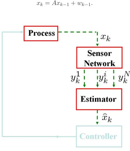
Consider the problem of state estimation over a wireless sensor network (Figure 3.1). The process dynamics is described by

xk=Axk−1+wk−1. (3.1)

Figure 3.1: State Estimation Using a Wireless Sensor Network

A wireless sensor network consisting of N sensors, i.e.,_{S1,· · ·, SN}, is used to measure

the state. WhenSi takes a measurement of the state in Eqn (3.1), it returns

y_ki =Hixk+vki, i= 1,· · · , N. (3.2)

In Eqn (3.1) and (3.2),xk∈IRnis the state vector,y_ki ∈IRmiis the observation vector for

Si,wk−₁ ∈IRnandv_ki ∈IRmi are zero-mean white Gaussian random vectors withE[wkwj′] =

δkjQ≥0,E[vi_kvit

′

] =δktΠi>0,E[vi_kvjt

′

] = 0_∀t, kandi₆=j,E[wkvit

′

] = 0_∀i, t, k. We assume that (A,√Q) is controllable, and (A, Call) is observable, where Call = [H1;· · ·;HN], i.e.,

the joint measurement matrix of all sensors.

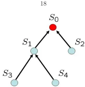
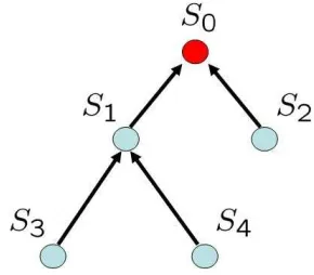
Figure 3.2: An Example of a Sensor Tree

we denote asS0, and consider a treeT with rootS0 (see Figure 3.2). We suppose that there

is a non-zero single-hop communication delay, which is smaller than the sampling time of the process. All sensors are synchronized in time, so the data packet transmitted from Si

to S₀ is delayed one sample when compared with the parent node of Si. We also assume

that Si aggregates the previous time data packets from all its child nodes with its current

time measurement into a single data packet. Therefore only one data packet is sent from Si to its parent node at each timek.

Let us define the following state estimate and other quantities at S₀ for a givenT:

ˆ

x−_k(T) , E[xk|all measurements up tok−1],

ˆ

xk(T) , E[xk|all measurements up tok],

P_k−(T) , E[(xk−xˆ−_k(T))(xk−xˆ−_k(T))′],

Pk(T) , E[(xk−xˆk(T))(xk−xˆk(T))′],

P∞(− T) , lim

k→∞P −

k (T),if the limit exists,

P∞(T) , lim

k→∞Pk(T),if the limit exists.

We drop the dependence on T, i.e., we write ˆx−_k(T) as ˆx−_k, etc., if there is no confusion on the underlyingT. In this chapter, we are interested in computing ˆxkand Pk for a given

3.3

Optimal Estimation Over a Sensor Tree

AssumeT has depthD. DefineYkk−i+1as the set of all measurements available at the fusion

center for timek₋i+ 1 at timek, i= 1,_{· · ·} , D. For the tree example in Figure 3.2, at time k, the fusion center has

Yk

k = {yk1, yk2},

Ykk−1 = {y 1

k−1, y2k−1, yk3−1, yk4−1}.

We immediately notice that Yk−i k−i ⊂ Y

k−i

k , i.e., more measurements for time k −i are

collected at kcompared with at timek₋i. For example,_Ykk−−₁1 ={yk1−₁, yk2−₁}are the only available measurements at time k₋1. However at time k, the available measurements for timek₋1 changes to _Ykk−1. Hence we can obtain a better estimate of xk−1 at timekthan

at time k₋1. This inspires us to recompute the optimal estimate of the previous states and use them as input to generate the current estimate. That is the basic idea contained in Theorem 3.1, where we recompute the optimal estimate ofxk−D+1,· · · , xk−₁ at time kand then make use of the updated estimates to compute the current estimate ˆxk. Figure 3.3

shows the overall estimation scheme at time k.

Let Sij be the node that is j hops away from S0. Define

Γj , [H1j;H2j;· · ·], j= 1,· · · , D

Ci , [Γ1;· · · ; Γi], i= 1,· · · , D

Υj , diag{Π1j,Π2j,· · · }, j= 1,· · · , D

Ri , diag{Υ1,· · · ,Υi}, i= 1,· · ·, D.

Intuitively, Γj is the joint measurement matrix and Υj is the joint noise covariance from

all sensors that are j hops from the fusion center. Ci is the joint measurement matrix,

and Ri is the joint noise covariance from all sensors that arej or less thanj hops from the

fusion center. With these definitions, the following theorem presents the optimal estimation algorithm over a sensor tree.

Figure 3.3: Kalman Filter Iterations at Time k

1. xˆk and Pk can be computed fromD Kalman filters as

(ˆxk−D+1, Pk−D+1) = KF(ˆxk−D, Pk−D,Y_kk−D+1, CD, RD)

.. .

(ˆxk−₁, Pk−₁) = KF(ˆxk−₂, Pk−₂,Y_kk−1, C₂, R₂) (ˆxk, Pk) = KF(ˆxk−₁, Pk−₁,Y_kk, C₁, R₁).

2. P∞− andP∞ satisfy

P∞− =gC2 ◦ · · · ◦gCD−1(P

∗

), (3.3)

P∞= ˜gC1 ◦gC2 ◦ · · · ◦gCD−1(P

∗

), (3.4)

where P∗

is the unique solution to gCD(P

∗ ) =P∗

.

DKalman filters stated in the theorem.

2) Follows directly from Eqn (2.14) and (2.15).

Remark 3.2 The estimation algorithm presented in Theorem 3.1 readily extends to a general graph that represents the sensor communications. The fusion center only needs to keep track of the measurement data up to previous time k₋D+ 1. Thus in a distributed setting, every node acts as a fusion center and the system robustness (against sensor failure) is increased.

3.4

Example

We consider an integrator chain in this section. The discrete time system dynamics is given by Eqn (3.1) with

A=





1 0.1 0 1



.

and with process noise covarianceQ= 0.3I. There are two sensors available. The measure-ment equations are given by

y1_k = [ 0 1 ]xk+vk1 =H1xk+vk1,

y2_k = [ 1 0 ]xk+vk2 =H2xk+vk2,

with covariances Π1 = 0.25 and Π2 = 0.5. Consider the following two sensor topologies

(Figure. 3.4).

P∗ =





0.1838 0.0103 0.0103 0.1822



,

which is the unique solution to P∗ =g_[H1;H2](P

∗

). As a result, for the star topology,

P∞(star) = ˜g_[H1;H2](P

∗ ) =





0.0825 0.0021 0.0021 0.0822



,

with Tr P∞(star)= 0.1647. For the line topology,

P∞(line) = ˜g_[H1](P

∗ ) =



 0

.1835 0.0047 0.0047 0.0823



,

with Tr P∞(line)= 0.2658.

0 5 10 15 20 25 30 35 40 45 50 −8 −6 −4 −2 0 2 k x k(1)

estimate from star topology estimate from line topology

0 5 10 15 20 25 30 35 40 45 50 0.1

0.2 0.3 0.4 0.5 0.6 0.7 0.8 0.9 1

Tr(P

k

)

k

KF over Star Topology KF over Line Topology

Figure 3.6: Error Covariances

We plot the first component of the true state and its estimates based on the two sensor topologies in Figure 3.5. We also plot the corresponding error covariance in Figure. 3.6. As those figures demonstrate, the simulations agree well with the theory developed.

3.5

Some Useful Inequalities

We conclude this chapter by presenting some useful inequalities that will be used in the next chapter.

Lemma 3.3 Assume 1_≤i_≤j _≤D and P _∈Sn

+. Then

≤



 Γ1

Γ2   ′_  

 Γ1

Γ2 

P



 Γ1

Γ2 



′ +R2





−_1

 Γ1

Γ2 



=



 Γ1

Γ2   ′_  B M

M′ G





−1  Γ1

Γ2 



whereB = Γ1PΓ′1+ Υ1,G= Γ2PΓ′2+ Υ2, and M = Γ1PΓ′2. Since B >0, G >0, and 



B M

M′ G



>0,

from Lemma 2.6, the Schur complement

SB ,B−M G−1M′ >0.

From Lemma 2.7, we obtain

  Γ1 Γ2   ′_  B M

M′ G





−_1

 Γ1 Γ2   =   Γ1 Γ2   ′_ 

X_{1 −}B−1_{M S}−1 B

−S_B−1M′B−1 S_B−1

    Γ1 Γ2  

= Γ′₁B−1Γ1+X2X2′

≥ Γ′₁B−1Γ1.

whereX1 =B−1+B−1M SB−1M

′

B−1 andX2 = Γ′1B

−₁ M S−

1 2

B −Γ

′

2S

−1 2

B . Having proved the

case i= 1, j = 2, the general case easily follows if we write Γ1:=Ci and Γ2 :=Cj \Ci.

Corollary 3.4 For all i= 1,_{· · ·}, n₋1, and all X_≥0,

Corollary 3.5 For all i= 1,_{· · ·}, n₋1, and all X_≥0,

˜

gCi+1(X)≤g˜Ci(X).

Chapter 4

Minimizing Sensor Energy

4.1

Introduction

Given a treeT that represents the sensor communications with the fusion center, we have seen in Chapter 3 how the optimal state estimate ˆxk can be computed at the fusion center,

and we have derived a closed form of the steady-state error covariance in Eqn (3.4). As stated in Chapter 1, the communication between the sensor nodes is limited, par-ticularly if nodes are located physically far way from each other. It takes time to transfer information from one node to another. Most nodes are battery powered, and hence to ex-tend the life time of such nodes, data are communicated over a multi-hop wireless network, instead of a single-hop network. The quality of the state estimate at the fusion center thus depends not only on the sensor quality but also on the communication delay, i.e., the num-ber of hops the sensor measurement data need to take until they reach the fusion center. Many short hops take longer time than a few long hops. On the other hand, a few long hops require larger transmission power since the required transmission grows rapidly with the distance between the wireless nodes. Hence, there is a trade-off between the state estimation quality and the overall energy cost. In this chapter, we consider the energy minimization subject to performance constraint.

the receiver node [5]. Some recent work addresses how to couple data routing with the sensing task using information theoretic measures [22].

The solution we propose is to optimize the network path for the sensor data via the

Tree Reconfiguration Algorithm such that the overall transmission energy is minimized, but guarantees a certain level of estimation quality. The resulting local sensor topology has the structure of a tree for which the fusion center is the root. In case sensor node failure happens, or new sensors join, or existing sensors leave to serve other applications, the tree can be reformed dynamically, which increases robustness of the overall system.

There are several potential application areas of the work presented in this chapter, including building automation, environmental monitoring, industrial automation, etc.

The rest of this chapter is organized as follows. After the mathematical framework is set up in Section 4.2, we state the energy minimization problem in Section 4.3, and propose the

Tree Reconfiguration Algorithm to minimize the energy usage of the sensors. The algorithm is presented in detail with a performance analysis. Examples are provided in the end to illustrate the algorithms developed.

4.2

Problem Set-up

Consider the problem of state estimation over a wireless sensor network (Figure 5.1).

xk=Axk−₁+wk−₁,

y_ki =Hixk+vki, i= 1,· · · , N.

For a tree T that represents the sensor communications with the fusion center (S0),

we have defined the estimation quantities [ˆxk(T), Pk(T), etc.] in Chapter 3.2. For the

remaining of this chapter, Node(T) means all the nodes of T, which is a subset of all sensors _{S1,· · · , SN}; FamT(Si) is the subtree of T that is rooted at Si; ParT(Si) is the

parent node of Si inT; Edge(T) is the edges of T, i.e.,

Edge(T),(Si, Sj) :Si∈Node(T), Sj = ParT(Si) .

Figure 4.2: Sensor Tree Example Revisited

Example 4.1 For the tree in Figure 4.2, we have that Node(T) =_{S1, S2, S3, S4}, FamT(S1) =

{S₃, S_4}, ParT(S3) =S1 and Edge(T) ={(S3, S1),(S4, S1),(S1, S0),(S2, S0)}.

Sometimes we write Si ∈ T to mean Si ∈ Node(T). For all notations, we drop the

Sensor Energy Cost Model

We assume that the sensor nodes are battery powered. Sensors spend energy in many ways, i.e., packet transmission and reception, idle listening, computing, etc. [13]. By using appropriate MAC protocol, e.g., the TDMA protocol, packet transmission and reception dominate the total energy usage. Given a treeT that represents the sensor communications withS₀, defineei

tx(T) as the energy cost forSi sending a measurement packet to its parent

node and ei_rx(T) as the energy cost for Si receiving a measurement packet from one of its

children, and we write ei_{(T) = e}i

tx(T) +eitx(T) as the total energy cost for Si in T. The

transmission power ei_tx(T) typically grows rapidly with the distance to the receiver. An estimate of ei

tx can be be computed based on the wireless technology. A common model

is that if the distance between Si and Par(Si) is di, then eitx = βi +αi(di)ni, where βi

represents the static part of the energy cost andαi(di)ni the dynamic part. The path-loss

exponent ni is typically between 2 and 6. The receiving energy eirx(T) is about the same

for each sensor, therefore without loss of generality, we write ei

rx(T) =erx. Then the total

energy cost of T per time is given by

e(T) = X

Si∈T

ei_tx(T) +_|T_|erx, (4.1)

where_|T_|denotes the number of sensor nodes inT.

4.3

Minimizing Sensor Energy

Problem of Interest

Since the sensors operate on batteries, it is natural to let the network operate at an energy level that is as low as possible. Thus we are interested in the following problem:

Problem 4.2 How should the tree T be established such that the total network energy cost is minimum yet the network provides a guaranteed level of estimation quality? i.e.,

min

T∈Tall e(T) subject to

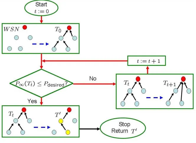
figuration Algorithm to approximate the optimal solution.

Tree Reconfiguration Algorithm

In this section, we present the Tree Reconfiguration Algorithm (Figure 4.3) which solves Problem 4.2 efficiently, but at the price of losing optimality in some cases.

Figure 4.3: Tree Reconfiguration Algorithm

TheTree Reconfiguration Algorithm (Figure 4.3) consists of three subroutines. The first subroutine is called by executing the Tree Initialization Algorithm to form an initial tree T₀ (the top rectangular block). Depending on whetherT₀ provides the required estimation quality, two other subroutines are called by executing the Switching Tree Topology Algo-rithm (the middle-right rectangular block) and the Minimum Energy Subtree Algorithm

Tree Initialization Algorithm

LetT0 denote the tree which represents the initial connection of the sensors with S0. T0 is

constructed via theTree Initialization Algorithm presented graphically in Figure 4.4.

Figure 4.4: Tree Initialization Algorithm: Intuitive Idea

The idea is that S0 first establishes direct connections with its neighbor sensors using

minimum transmission power level ∆e. After that, its neighbor sensors establish further connections with their own neighbor sensors also using minimum transmission power level ∆e. This process continues until a tree of depthDis formed. LetS(t) be the sensors added to T₀ at or before step t, ∆S(t) be the set of sensors added at step t, and V_∆e(Si) be the

set of sensors that are reachable by Si using ∆eenergy. The Tree Initialization Algorithm

is presented in its flow diagram form in Figure 4.5 with

V∆e(Σ), [

Si∈Σ

V∆E(Si).

Switching Tree Topology Algorithm

For a given tree Tt, if P∞(Tt) Pdesired, the tree needs to be adjusted in a way that the

estimation quality is improved. The Switching Tree Topology Algorithm provides such a way (Figure 4.6).

We defineπ(Tt, Si) as the operation thatSibreaks connection with Par(Si) and connects

directly to S₀, i.e., Node π(Tt, Si)

= Node(Tt) and

Edge π(Tt, Si)= Edge(Tt) [

{Si, S0} \ {Si,ParTt(Si)}.

Further define S2hop , {Si ∈ Tt : Par(Par(Si)) = S0}. The algorithm is then given as

Figure 4.5: Tree Initialization Algorithm: Flow Diagram

Algorithm 1 Switching Tree Topology Algorithm Init: Tt.

Compute

Sp = arg min Si∈S2hop

P∞(π(Tt, Si)).

Return Tt+1 :=π(Tt, Sp).

Minimum Energy Subtree Algorithm

For a given tree T with P∞(T) ≤ P_desired, the Minimum Energy Subtree Algorithm finds the subtreeT′ rooted atS0 with the property thatP∞(T′)≤Pdesired, and e(T′)≤e( ˜T) for

any subtree ˜T ofT rooted atS0. The idea is that all possible subtrees ˜T rooted atS0 and

satisfying

P∞( ˜T)_≤Pdesired

are found in an efficient way utilizing the structure of T. Then the subtree T′ which has the least overall energy cost is returned. The details are as follows.

To make the presentation clear and easy to follow, we divide the algorithm into several key steps and provide an example to illustrate each step. Before introducing the algorithm, let us define

S(i1i2· · ·ip) , {Si1, Si2,· · ·Sip},

Ω(i1i2· · ·ip) , T\S(i1i2· · ·ip),

where it is assumed i1 ≤i2 ≤ · · · ≤ip. We consider the following example to demonstrate

the algorithm.

Figure 4.7: TreeT and Some Subtree ˜Ts

Example 4.3 Consider the tree T with four sensor nodes in Figure 4.7. Assume the following:

1) T provides enough estimation quality, i.e.,P∞(T)≤P_desired. 2) No single sensor provides enough estimation quality, i.e.,

P∞(S(i))Pdesired, i= 1,2,3,4.

3) Among the two sensor pairs, only _{S1, S4} can provide enough estimation quality,

i.e.,

5) The energy cost of single hop communication is ∆e.

By the above assumptions, it is easy to see that the minimum energy subtreeT′ is given by ˜T4 withe( ˜T4) = 2∆e.

Let us examine the case when we take T as an input to theMinimum Energy Subtree Algorithm which consists of the following key steps.

Step 1 • Init: T

• l:= 0,_Dl :={Sip ∈T :P∞(Ω(ip))≤Pdesired}.

In this step, _D0 holds all single-sensor nodes without which the remaining sensors still

satisfy the accuracy requirement. Therefore in Example 4.3,D0 ={S2, S3, S4}.

Step 2

• l:=l+ 1,_Dl:=Dl−₁

• ∀Sip∈ Dl−1 withP∞(Ω(ip))≤Pdesired

- _∀q > p andSiq 6∈Fam(Sip),

ifP∞(Ω(ipiq))≤Pdesired,Dl:=DlSS(ipiq).

In this step, _D1 holds all single-sensor or two-sensor pairs without which the remaining

sensors still satisfy the accuracy requirement. The third line of step 2 eliminates the redun-dancy in listing the subtrees as S(ipiq) =S(iqip), and if Sip is removed from a tree, so is

Step 3

• l:=l+ 1,_Dl:=Dl−₁

• ∀S(ipiq)∈ Dl−1 with P∞(Ω(ipiq))≤Pdesired

- _∀o > q and Sio 6∈(Fam(Sip)

S

Fam(Siq)),

ifP∞(Ω(ipiqio))≤Pdesired,

Dl:=DlSS(ipiqio).

Similar to step 3, _D2 holds all single-sensor, two-sensor pairs or three-sensors without

which the remaining sensors still satisfy the accuracy requirement. The algorithm continues in this way until _Dr =Dr−₁ at some step r≤D.

Step r+1

• Return T′= arg min_Ω(·)∈De(Ω(·))

In Example 4.3, D2 ={S2, S3, S4, S(23)}=D1. Hence the algorithm stops and returns

T′ = Ω(23) =S(14) = ˜T4 with P∞(T′)≤Pdesired and e(T′) = 2∆e.

Performance Analysis of the Algorithms

The performance of the Tree Reconfiguration Algorithm is summarized in the following theorem.

Theorem 4.4 (1) Given a tree Tt, the Switching Tree Topology Algorithm returns Tt+1 ∈

Tall such that

P∞(Tt+1)≤P∞(Tt).

(2) Given a tree T with P∞(T) _≤ Pdesired, the Minimum Energy Subtree Algorithm

returns T′ _⊂T rooted at S0 such that

P∞(T′)≤Pdesired ande(T

′

)≤e( ˜T)

extend the proof for a general tree. For Tt,P∞(Tt) is given by Eqn (3.4) as

Figure 4.8: Switching Tree Topology

P∞(Tt) = ˜gC1 ◦gC2 ◦gC3 ◦ · · · ◦gCD−1(P

∗ ),

whereP∗

≥0 is the unique solution to

gCD(P

∗

) =P∗.

ForTt+1, P∞(Tt+1) is given by

P∞(Tt+1) = ˜gC2 ◦gC3 ◦gC4◦ · · · ◦gCD−1(P

∗ ) = ˜gC2 ◦gC3 ◦gC4◦ · · · ◦gCD−1 ◦gCD(P

∗ ) ≤ g˜C1 ◦gC2 ◦gC3◦ · · · ◦gCD−2 ◦gCD−1(P

∗ ) = P∞(Tt)

where the inequality is from Corollary 3.4 and 3.5. (2) Suppose T∗

= (S∗_,

Edge(T∗

∆S_{⊂ D}r, asP∞(T∗)≤Pdesired. We also haveS(i1i2)∈ Dr as

P∞(T_\S(i1i2))≤P∞(T∗)≤Pdesired.

Similarly, S(i1i2· · ·im) ∈ Dr and so T∗ = T \S(i1i2· · ·im) is returned by the Minimum

Energy Subtree Algorithm as we assume T∗ is the subtree that has the least energy cost. (3) LetT⋆ denote the star tree, i.e., all sensors communicate withS0 directly. It is easy

to verify thatP∞(T⋆)≤P∞(T) for allT _{∈ Tall}. If there existsT such thatP∞(T)≤P_desired, we must also have P∞(T⋆) _≤ P∞(T). Suppose at t1, P∞(Tt1) ≤ Pdesired, then it is clear

that P∞(T′) ≤ P_desired. Otherwise, the Tree Reconfiguration Algorithm continues until direct connections between all sensors with S0 are established, in which case P∞(Tt) =

P∞(T⋆)≤P_desired. HenceP∞(T′)≤P_desired.

A TDMA Scheduling Scheme

In this section, we present a TDMA scheduling scheme for practical implementation of the Tree Reconfiguration Algorithm, which is similar to the scheduling phase in [10]. Assume each discrete time is divided into some equal length time slots, e.g., in wireless HART protocol [19], there are 100 time slots per second. The advantage of TDMA scheme is that sensors only need to communicate during its own time slot and hence save energy by avoiding the idle listening. The scheme consists of the following two phases.

1. The fusion center calculates the (Si,Par(Si)) pair according to the Tree

Reconfigura-tion Algorithm. It then assigns one time slot to each (Si,Par(Si)) pair, i.e., Si will

communicate with Par(Si) at the specified time slot.

2. At the beginning of every M times, the fusion center broadcasts the communication schedule to all sensors.

Figure 4.9: Different Trees Formed by the Tree Reconfiguration Algorithm

schedule based on the remaining sensors and broadcasts the new schedule at the beginning of the next cycle. Similarly, new sensors might join the network for the same or different applications. The fusion center can again calculate and broadcast the new schedule.

4.4

Examples

Three sensors are available to measure the state of a process (see Figure 4.9). Assume that ifSi is connected toSi−₁, i= 1,2,3, the energy of communication is ∆e; ifSi is connected

toSi−₂, i= 2,3, the energy is 4∆eand ifS₃ is connected toS₀, the energy is 8∆e. Without loss of generality, for the remaining of the examples, we only calculate the total transmitting energy. We consider two scenarios in this section.

Tree Reconfiguration with Time-Varying Disturbances

The discrete time system dynamics is given by Eqn (3.1) with

A=



      

1 0.1 0.05 0.0002 0 1 0.1 0.05 0 0 1 0.1

0 0 0 1



      

The measurement equations for the three sensors are given by

y_k1 = [ 1 0 0 0 ]xk+v1k,

y_k2 = [ 0 1 0 0 ]xk+v2k,

y_k3 = [ 0 0 1 0 ]xk+v3k,

with Π1 = 0.25,Π2 = 0.5, and Π3 = 0.5. AssumeSi isihops away from S0 (Figure 4.9).

The dynamics in the simulation include control input as well, i.e., xk=Axk−₁+Buk+

wk−1, which is computed via the standard LQG control procedures. In this example B =

[0 0 0 1].

Suppose it is required that Tr(P∞) _≤ 10 for this system. Notice that we can simply replace P∞ ≤ P_desired with Tr(P∞) ≤ Tr(P_desired) in all previous algorithms. Initially, assumeQk=Q0 ,0.2I for allk≤k1 = 200. AfterT0 is set up,S0 computes Tr(P∞(T0)) =

4.1297<10. Thus it starts to run theMinimum Energy Subtree Algorithm to find outT′. In this case T′ =T0\S3 with Tr(P∞(T′)) = 9.6411 ande(T′) = 2∆e.

We model the disturbance to the plant as changes to Qk. Suppose at time k1 + 1,

Qk changes to 4Q0 and will last for 100 time steps. We assume the changes in Qk are

known to S0. In the actual implementation, we can estimate the value ofQk using various

available schemes (e.g., see [31]). In this case, T0\S3 no longer provides enough accuracy

as Tr P∞(T′) changes to 34.9300. Thus S0 executes the Tree Reconfiguration Algorithm

again to find the desired tree. Now only the star topology T₂, with Tr(P∞(T₂)) = 9.6369, provides enough accuracy. The price to pay for reconfiguring to T2 is that e(T2) = 13∆e.

Figure 4.11 shows how the different tree locations change in the energy-error diagram for these scenarios. Later whenQkchanges back toQ0 atk2 = 300,T2 is reconfigured toT0\S3

correspondingly.

Figure 4.10 shows the evolution of the fourth component ofxkand the estimation error

ekwithout and with the tree reconfiguration. As we can see from the lower half of the figures,

0 200 400 600 800 −50

k

0 200 400 600 800 −50

0 50

k

xk

4

T0 − S3 T2

0 200 400 600 800 −15

k

0 200 400 600 800 −15

−10 −5 0 5 10 15

k

ek

4

T0 − S3 T2

Figure 4.10: x4_k and e4_k without/with Tree Reconfiguration

Figure 4.11: Changes of Tree Locations in Energy-Error Diagram

Tree Reconfiguration with Time-Varying Performance Requirement

In this example, the dynamics of the process and sensor measurement equations are as follows:

xk = 0.9xk−1+wk−1,

y_k1 = xk+vk1,

y_k2 = xk+vk2,

with Q = 1,Π1 = 1.5,Π2 = 1, and Π3 = 0.5. Suppose the following performance

require-ment is received by the fusion center:

P∞ ≤ 0.75,1≤k≤100, P∞ ≤ 0.25,101≤k≤200, P∞ ≤ 1.0,201 ≤k≤300, P∞ ≤ 0.75,301≤k≤500.

Then the fusion center can find the corresponding minimum energy tree that fulfills the performance requirement. The intuitive idea is presented in Figure 4.12.

Figure 4.12: Tree Reconfiguration with Time-Varying Performance Requirement

Figure 4.13 shows the simulation result when the fusion center uses the same tree (T0_\S3) all the time, and when it reconfigures the trees according to the performance

Chapter 5

Maximizing Network Lifetime

5.1

Introduction

In the previous chapter, we study the problem of minimizing sensor energy usage when considering estimation over a sensor network. In this chapter, we study the lifetime max-imization problem. Sensor network lifetime maxmax-imization problem has been a hot area of research over the the past few years, as one of the critical constraints of such networks is limited energy resources available. Xue and Ganz [56] showed that the lifetime of the sensor networks is influenced by transmission schemes, network density and transceiver parameters with different constraints on network mobility, position awareness and maximum transmis-sion range. Chamam and Pierre [8] proposed a sensor scheduling scheme to optimally put sensors in active or inactive modes. A sensor transmitting scheduling was suggested by Chen et al. [9]. Lai et al. [26] proposed a scheme to divide the deployed sensors into disjoint subsets of sensors such that each subset can complete the mission, and then maximized the number of such disjoint subsets. Similar approaches can be found in [36] where the sensors are partitioned into groups which are successively scheduled to be active for sensing and delivering data.

The solution we propose is to construct a set of sensor trees which all provide the guar-anteed estimation quality and then schedule those sensor trees appropriately to maximize the lifetime of the whole network.

Figure 5.1: State Estimation Using a Wireless Sensor Network

Again consider the problem of state estimation over a wireless sensor network (Fig-ure 5.1). The process dynamics, sensor meas(Fig-urement equations and sensor energy models are the same as in Section 4.2, i.e.,

xk=Axk−₁+wk−₁,

y_ki =Hixk+vki, i= 1,· · · , N,

and the total energy cost of a treeT is

e(T) = X

Si∈T

ei_tx(T) +|T_|erx.

A Motivating Example

Example 5.1 Consider the following network with N = 2. Assume both T₁ and T₂ in Figure 5.2 satisfy

Further assume that

P∞(Si)Pdesired, i= 1,2.

Let eij be the total energy cost for Si in Tj, i, j = 1,2, and let Ei be the initial energy for

Si. Consider the following parameters.

E = [eij] = 

 10 1

1 10



,E₁=E₂ = 1000.

Figure 5.2: Network with Two Sensors

If we measure the lifetime of the network (denoted as L) as the first time that a sensor dies due to running out of battery, then it is easy to see that L = 100 when the Tree Reconfiguration Algorithm is executed, as T₁ is the only tree used.

It turns out that we can increase L by mixing the use of T1 and T2. Let 0 ≤ α ≤ 1

denote the portion of times that T₁ is used, we can show that if 0< α <1, then L >100. It is also easy to verify that Lattains its maximum value at 181 when α = 0.5.

Θ,{θ:Z → Tall}.

Let θ(k) =T_kθ _{∈ T}all. As θ(k) determines the energy consumed by Si at k, given an initial

energy levelEi forSi,Lcan be calculated usingθ. We are interested in finding a scheduling

policyθsuch thatLis maximized. We also require that the estimation quality at the fusion center reaches certain desired level. In mathematical form, we are interested in solving the following network lifetime maximization problem

max

θ∈_ΘL(θ) subject to

P∞(T_kθ)_≤Pdesired.

Let _Td−depth denote the set of trees which have depthd. Then it is easy to see that

|Tall| = N X

d=1

|Td−_depth| > _|T2−_depth| =

N−1 X

j=1 



N

j



jN−j.

For example, when N = 10, _|T2−depth| ≈ 2.24×106, therefore it is computationally

in-tractable to consider all trees in_Tall and all scheduling policies in Θ when N is large. We

thus propose the following two steps to approximate the optimal solution to the network lifetime maximization problem.

Step 1: Construct an appropriate_{T ⊂ T}all.

Step 2: Schedule_T appropriately.

restricting θ on _T. As _T is only a subset of _Tall, the resulting θ∗ may not be globally

optimal in general. In the next few sections, we give details for the above two steps.

5.3

Constructing and Scheduling Sensor Trees

Step 1: Construct Sensor Trees

The proposed Tree Construction Algorithm consists of three main subroutines which are the Random Initialization Algorithm, the Topology Improvement Algorithm and the Tree Reconfiguration Algorithm. The overall algorithm is presented in Figure 5.3.

Figure 5.3: Tree Construction Algorithm

Random Initialization Algorithm

Define the following quantities:

Sj−hop , {Si :Si is j−hop away from S0},

Sc(T) _{, {}Si :Si is not in T}.

The intuitive idea of the Random Initialization Algorithm is thatSj−hop, j= 1,· · ·, D are

while (_{S 6}=_∅)do D:=D+ 1

Pick nD from (1,|Sc|) uniformly randomly.

l:= 1

while (l_≤nD) do

Pick anySp ∈ Sc and any Sq∈ S(D−1)−hop uniformly randomly.

ConnectSp to Sq.

Sc _:=Sc_{\ {S} p}

T :=T _{∪ {}Sp,(Sp, Sq)}

SD−hop :=SD−hop∪ {Sp}

l:=l+ 1 end while end while

After the execution of the Random Initialization Algorithm, an initial tree of depth D is constructed with|Sj−hop|=nj, j= 1,· · ·, D, andPDj=1nj =N.

Remark 5.2 Ifn1 =N, then the algorithm returnsT⋆, i.e., all sensor nodes connect toS0

directly.

Topology Improvement Algorithm

Since the previous algorithm randomly constructs the initial tree, some sensor communica-tion paths may be established inefficiently, i.e., some sensors use more energy yet need more hops to communicate withS0. The Topology Improvement Algorithm aims to remove this

inefficiency.

When Si is connected to Sp, we define τip as the number of hops between Si and S0,

and eip as the transmission energy cost of Si. Similarly we define τi0 and ei0 for Si in the

initial tree constructed by the Random Initialization Algorithm.

We consider modifying the path of Si in the initial tree, whereSi ∈ Sj−hop, j ≥2, only

if there exists Sp in the same tree and Sp ∈ Sj−_hop, j ≤ τi0−1 such that either eip < ei0

or eip = ei0 and τip < τi0. In these cases, Si is connected to Sp. The first condition

corresponds to reducing the energy cost of Si yet not making the hops between Si and S0

yet not increasing its energy cost. DefineFi as the indicator function forSi, where Fi = 1

means that Si has already been examined for possible improvement andFi = 0 otherwise.

The full algorithm is presented below.

Algorithm 3 Topology Improvement Algorithm ∀i Fi := 0

∀Si∈ Sj−hop, j≤1, Fi := 1

while _∃Fi= 0 do

Fi:= 1

Σ :=_{Sp :Sp ∈ Sj−hop, j≤τi0−1, eip≤ei0}

if Σ₆=_∅ then

τiq := min{τip:Sp ∈Σ}

if eiq< ei0 or (eiq =ei0 and τiq< τi0) then

reconnect Si to Sq

update Sj−hop, j≤τi0

end if end if end while

Notice thatFi is set to be 1 for allSi ∈ Sj−hop, j≤1, as for those sensor nodes that are

one hop away from S0, no improvement can be made that further reduces the energy cost

(and maintains the same hop numbers) or reduces the hop numbers.

At this step, we have constructed a set ofM randomized initial trees. We then use them as input to the Tree Reconfiguration Algorithm presented in Section 4.3 to make sure that each tree provides the desired estimation quality.

Step 2: Schedule Sensor Trees

The Random Initialization Algorithm and Topology Improvement Algorithm aim to create a set of sensor trees_T with different energy cost of individual sensors (due to the randomness). The Tree Reconfiguration Algorithm changes the resulting sensor trees and guarantees that for all Tj ∈ T,

P∞(Tj)≤Pdesired.

Denote eij as the total energy cost (transmission and receiving energy) forSiinTj, and

tj(θ) as the time that Tj is used for a policy θ, so the network lifetime L(θ) is given by

L(θ) =

M X

j=1

subject to

m X

j=1

tjeij ≤Πi, i= 1,· · · , N

tj ≥tmin, j = 1,· · · , M

wheretj ≥tmin is added to make sure the estimation process enters steady state after some

transient period. This problem can be solved efficiently via linear programming, as both the objective function and constraints are linear functions of the variables.

5.4

Examples

In this section, we provide an example to demonstrate the theory and algorithms developed so far. We start by describing the process and sensor models.

Process and Sensor Models

We consider the process in Eqn (3.1) with

A=



      

1 0.1 0.05 0.0002 0 1 0.1 0.05 0 0 1 0.1

0 0 0 1



      

,

and Q= 0.1I. There are three sensors available. The measurement equations are given by

y_k1 _{= [ 1 0 0 0 ]}xk+v1k,

y_k2 _{= [ 0 1 0 0 ]}xk+v2k,

with Π1 = 0.5,Π2 = 0.25, and Π3 = 0.1. Assume the sensors are placed in a line (Figure 5.4)

with relative distance

d₁₀= 2, d₂₁= 1, d₃₂= 1, wheredpq is the distance betweenSp and Sq.

Figure 5.4: Initial Sensor Topology

Let etx(Sp, Sq) be the energy cost for Sp transmitting a packet to Sq and erx(Sp, Sq)

be the energy cost for Sq receiving such a packet fromSp. We use the following simplified

energy model

erx(Sp, Sq) = 1, etx(Sp, Sq) =d2pq,∀1≤p, q≤3, p6=q.

Assume the initial energy_Ei available atSi is known and given by

E1=E2 =E3= 2000.

Tree Construction Algorithm

Let the performance specification at the fusion center be

Tr(P∞(Tk))≤2.5∀k.

We pick M = 4 for this example. Figure (5.5)–(5.8) demonstrate the use of the Tree Construction Algorithm. As a result,

T ={T1, T2, T3, T4}

is returned with



5 1 16



Notice that during the construction of T1, only the Switching Tree Topology Algorithm

modifies the input tree. ForT2andT4, only the Topology Improvement Algorithm modifies

the input tree. For T₃, both the Topology Improvement Algorithm and the Minimum Energy Subtree Algorithm modify the input tree.

Figure 5.5: Tree 1

Figure 5.7: Tree 3

Figure 5.8: Tree 4

Tree Scheduling Algorithm

Using the notations in Section 5.3, lettjbe the time thatTj will be used. Assumetmin = 20.

In order to maximize the lifetime of the network, we solve the following scheduling problem:

max

tj

4 X

j=1

tj

subject to

4 X

j=1

tjeij ≤2000, i= 1,2,3

tj ≥20, j= 1,2,3,4.

Define the following quantities

z _, [t1 t2 t3 t4]′,

f _, [₋1 ₋1 ₋1 ₋1]′, Φ ,





E′ −I



,

subject to

Φz_≤b

which can be easily solved via standard LP toolbox. The following optimal value of z is obtained as a result1:

z∗ = [150 20 20 94], and the maximum network lifetimeL∗ is given by

L∗=−f′z∗ = 284.

Let L(j) denote the lifetime of the network whenTj is always used. It is easy to compute

that

L(1) = 200, L(2) = 181, L(3) = 222, L(4) = 125,

and hence the network lifetime is indeed enhanced by the Tree Scheduling Algorithm.

True and Computed Error Process

In the previous section, we calculate the optimal scheduling policy for _T. We then run a Monte Carlo simulation based on the optimal time that Tj is used. Figure 5.9 shows the

average Pk and ||ek||2 as a result of 1000 runs. The performance specification is clearly

satisfied.

1

0 50 100 150 200 250 300 0.8

1 1.2 1.4 1.6 1.8 2 2.2 2.4 2.6

k

Tr(P_k)

||e

k|| 2

T

3 T1 T2 T4

Chapter 6

Minimizing Buffer Length

6.1

Introduction

The Kalman filter has played an important role in system theory and has found wide ap-plications in many fields, such as control, signal processing, and communications. In the standard Kalman filter, it is assumed that sensor data are transmitted along perfect com-munication channels and are available to the estimator either instantaneously or with some fixed delays, and no interaction between communication and control is considered. This ab-straction has been adopted until recently when networks, especially wireless networks, are used in sensing and control systems for transmitting data from sensors to controller and/or from controller to actuator. While having many advantages such as low cost and flexibility, networks also induce many new issues due to their limited capabilities and uncertainties such as limited bandwidth, packet loss, and delay. On the other hand, in wireless sensor networks, sensor nodes also have limited computation capability in addition to their limita-tions in communicalimita-tions. These constraints undoubtedly affect system performance or even stability and cannot be neglected when designing estimation and control algorithms, which has partially inspired this thesis work. We devote this chapter to the study of Kalman filtering over a packet delaying network.

investi-gated in [40, 48, 51] via the linear matrix inequality and the Riccati equation approaches, respectively. We study the problem from a probabilistic angle, which is different than most existing approaches.

The probability distribution of the delay is assumed to be given and we aim to give a complete characterization of filter performance. Due to the limited computation capability of the filtering center, and also in consideration of the fact that a late-arriving measurement related to the system state in the far past may not contribute much to the improvement of the accuracy of the current estimate, it is practically important to determine a proper buffer length for measurement data within which a measurement will be used to update the current state and beyond which the data will be discarded.

The buffer provides a tradeoff between performance and computational load. In this chapter, for a given buffer length, we give lower and upper bounds for the probability at which the filtering error covariance is within a prescribed bound, i.e., Pr[Pk≤M] for some

given M. The upper and lower bounds can be easily evaluated by the probability distri-bution of the delay and the system dynamics. An approach for determining the minimum buffer length for a required performance in probability is given, and an evaluation on the number of expected filter updates is provided. Both the cases of sensor with and without necessary computation capability for filter updates are considered.

6.2

Problem Setup

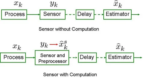
System Model

We consider the networked control systems shown in Figure 6.1, where a sensor measures the current state of a process and sends the measurement data (or preprocesses the data and sends its local estimate of the state) via a packet delaying network to a remote estimator.

The process dynamics and sensor measurement equation are given as follows:

xk = Axk−1+wk−1, (6.1)

yk = Cxk+vk. (6.2)

In the above equations, xk ∈ IRn is the state vector, yk ∈ IRm is the observation vector,

ˆ

xs_k,E[xk|y1,· · ·, yk].

The two cases correspond to the two scenarios in Figure 6.1, i.e., sensor without/with computation capability.

Network Delay Model

After taking a measurement at time k, the sensor sends yk (or ˆxsk) to a remote estimator

for computing the state estimate. We assume that the measurement data packets from the sensor are to be sent across a packet delaying network, with negligible quantization effects, to the estimator. Each yk (or ˆxs_k) is delayed by dk times, where dk is a random variable

described by a probability mass function f, i.e.,

f(j) =Pr[dk=j], j = 0,1,· · ·. (6.3)

For simplicity, we assume dk1 and dk2 are inde