Volume 2011, Article ID 753572,13pages doi:10.1155/2011/753572
Research Article
A Signal-Specific QMF Bank Design Technique Using
Karhunen-Lo´eve Transform Approximation
Muzaffer Dogan
1and Omer N. Gerek
21Department of Computer Engineering, Anadolu University, IkiEylulKampusu, 26470 Eskisehir, Turkey
2Department of Electrical and Electronics Engineering, Anadolu University, IkiEylulKampusu, 26470 Eskisehir, Turkey
Correspondence should be addressed to Muzaffer Dogan,muzaff[email protected]
Received 31 July 2010; Revised 3 December 2010; Accepted 5 January 2011
Academic Editor: Antonio Napolitano
Copyright © 2011 M. Dogan and O. N. Gerek. This is an open access article distributed under the Creative Commons Attribution License, which permits unrestricted use, distribution, and reproduction in any medium, provided the original work is properly cited.
Block Wavelet Transforms (BWTs) are orthogonal matrix transforms that can be obtained from orthogonal subband filter banks. They were initially generated to produce matrix transforms which may carry nice properties inheriting from wavelets, as alternatives to DCT and similar matrix transforms. Although the construction methodology of BWT is clear, the reverse operation was not researched. In certain cases, a desirable matrix transform can be generated from available data using the Karhunen-Lo´eve transform (KLT). It is, therefore, of interest to develop a subband decomposition filter bank that leads to this particular KLT as its BWT. In this work, this dual problem is considered as a design attempt for the filter bank, hence the wavelets. The filters of the decomposition are obtained through lattice parameterization by minimizing the error between the KLT and the BWT matrices. The efficiency of the filters is measured according to the coding gains obtained after the subband decomposition and the experimental results are compared with Daubechies-2 and Daubechies-4 filter banks. It is shown that higher coding gains are obtained as the number of stages in the subband decomposition is increased.
1. Introduction
In signal coding, subband decomposition and block trans-formation are popularly used in signal compression [1,2]. In both methods, the signal is projected to subspaces with better (more efficient) representation properties. In the transform domain, the coefficients are usually coded by nonuniform bit allocation depending on the energy distribution.
The relation between discrete wavelet transform (imple-mented by subband decomposition [3, 4]) and matrix transforms is also known [5]. Particularly, orthonormal transform matrices can be obtained by iteratively applying shifted impulse trains (with certain periods) and observing the constant output of the balanced subband decomposition tree, as described inSection 2.
Karhunen-Lo´eve transform (KLT) is a matrix transform constructed specifically for a group of signals with certain covariance characteristics. It is then efficiently used for several applications such as feature extraction. Although orthogonal matrices (BWTs) can be obtained from subband-based multiresolution signal decomposition [5], the analysis
of how to obtain the filter coefficients of a subband filter bank that generates a desired transform matrix is lacking. An attempt to obtain subband decomposition filters that lead to an efficient (e.g., KLT) matrix as its BWT is believed to serve well in the area of wavelet design.
The mapping from subband decomposition representa-tion to BWT is many-to-one. Therefore, the search for a filter bank that satisfies a certain BWT requires several other conditions, and the solution is not unique.
Akkarakaran and Vaidyanathan [6] proved that the KLT matrix is a principal component filter bank for a given class Cof orthonormal uniformM-channel filter banks. However, they do not propose a method to obtain the (sub-)optimum filter bank in cases where the KLT matrix is not included
inC. The class of BWT filter banks, sayC(BWT), is a subset
4↓
4↓
4↓
4↓
u1(n)
u2(n)
u3(n)
u4(n) x(n)
H0(ω)
H1(ω)
H2(ω)
H3(ω)
(a)
x(n)
2↓
2↓
2↓
2↓
2↓
2↓ u11(n)
u12(n)
u21(n)
u22(n)
u23(n)
u24(n) H0(ω)
H0(ω)
H0(ω) H1(ω)
H1(ω) H1(ω)
(b)
Figure1: Decomposition structures: (a) 4-channel decomposition, (b) two-stage subband decomposition.
C
C(BWT)
KLT
(a)
C
C(BWT)
KLT
(b)
Figure2: A sketch ofM-channel filter bank class,Cand its dyadic BWT subset,C(BWT). (a) KLT inC. (b) KLT not inC.
(last filter is computed using the orthonormality con-straints). Therefore, due to a greater degree of freedom, the 4-channel decomposition has a higher probability to reach closer to KLT. Figure 2 roughly sketches C and C(BWT). It is proved in [6] that the KLT is the optimum filter bank if C contains it. In case where the KLT is not included inC, no solution is proposed for the optimum filter bank. In this work, the inability of [6] to produce “close to KLT” results is handled together with the limitation of dyadic and repeated processing of 2 channel filter banks to produce BWT.
The lattice parameterization method can be used to decrease the number of free parameters of a QMF bank and the filter coefficients can be expressed in terms of trigono-metric functions of the angle parameter. This effectively reduces the search space of the filter coefficients down to less number of angle terms. Here, the BWT decomposition is reversed so that a desired matrix, the KLT, is obtained using quadrature mirror filters in iterations of 2-channel decompositions. The motivation of the study is the possi-bility that the KLT matrix (or a matrix that is close) can be obtained by BWT decomposition since both the KLT matrix and the BWT matrix are orthonormal matrices. Although the channel decomposition structure inFigure 1(a)can be used in this process, the BWT structure inFigure 1(b)is preferred because the number of filters to be optimized is less in the iterated 2-channel BWT structure.
The proposed design method here is a filter bank design method which uses a given block transform matrix (the KLT matrix) as the optimization function, and it is least squares optimal with respect to the autocorrelation, while
x(n)
2↓
2↓
2↑
2↑
H0(z)
H1(z)
F0(z)
^
x(n)
u1(n)
u2(n)
+
F1(z)
Figure3: A two-channel QMF bank.
previous methods (i.e., [6]) seek for an optimization through similarity to a set of basis functions. Thus, the adopted strategy may provide an insight and arise an interest in this new design approach.
A numerical search algorithm that provides finite extent quadrature mirror filters (QMFs) was previously studied [7] and the performance of QMF banks obtained from KLT matrices of size 4×4 are compared with Daubechies-2 filter banks [8]. In this paper, the method proposed in [8] is improved and it is extended to 8×8 KLT matrices obtained from row- and column-KLT matrices of several test images.
In the following sections, BWT, KLT, and the lattice parameterization will be explained briefly. Then, the pro-posed method,BWT Inversion, will be developed analytically for the 4×4 case and experimentally for the 8×8 case. The efficiency of the generated filter banks will be compared with Daub-2 and Daub-4 filter banks by using the coding gain expression. Finally, the conclusion and the future works will be discussed.
2. Block Wavelet Transform
Figure 1(b)shows the two-stage subband decomposition tree. Here, the approximation and detail signals obtained from one-stage decomposition are decomposed by using the same filters and four subsignals are obtained.
The framework of BWT states that, using the scheme in Figure 3, a transform matrix of size 2×2 can be generated, and usingFigure 1(b), a transform matrix of size 4×4 can be generated. In general, iflstages are considered (meaning that there areN=2lsubbands), then a transform matrix of sizeN×Ncan be generated.
The BWT matrix of size 2×2 is generated by applying two 2-periodic signals, x1[n] and x2[n] whose samples in one period are [0, 1] and [1, 0], respectively, to the system shown in Figure 3. Indeed, x2[n] is the shifted version of
x1[n]. Whenx1[n] andx2[n] are convolved withh0[n] and
h1[n], the resultant signals are also 2-periodic. If these signals are down-sampled by 2, 1-periodic signals are obtained in the sub-bands. The samples which repeat themselves are the sub-band signals construct the BWT matrix.
For the 4×4 case, four 4-periodic signals, x1[n],
x2[n], x3[n], and x4[n] whose samples in one period are [1, 0, 0, 0], [0, 1, 0, 0], [0, 0, 1, 0], and [0, 0, 0, 1] are applied to the two-stage decomposition structure shown in Figure 1(b). Convolving each input signals withh0[n] and
h1[n] and then down-sampling the results by two gives 2-periodic signals. Convolving the output signals of the first stage by h0[n] and h1[n] and down-sampling by 2 yields 1-periodic signals at the end of the second stage. The repeating samples construct the 4×4 BWT matrix. The four repeating samples obtained when x1[n] is applied to the system construct the first column on the BWT matrix; the repeating samples for the case whenx2[n] is applied to the system construct the second column of the BWT matrix, and so on.
In general case ofN×N, whereNis a power of 2, that is,N=2l,Ninput signals each of which areN-periodic are applied to thel-stage decomposition tree and the repeating samples of the sub-band signals obtained after the last stage of the structure construct the BWT matrix.
BWTs that are obtained in this manner are orthogonal transforms, that is, ANTAN = IN where AN is the BWT matrix of sizeN×NandIN is theN×Nidentity matrix and the matrix coefficients can be computed by fast (O(NlogN)) algorithms [5].
When the input signals of sizeN×1, used for computing the BWT matrix, are written into the columns of anN×N
matrix, the identity matrix is obtained. It is shown that the BWT matrix remains orthogonal when any orthonormal input vectors are used as the input signals [9]. It means that using−1 instead of 1 in any input signal does not affect the orthogonality of the BWT matrix, but it changes the signs of the elements of the corresponding row.
Eigenvector matrices, such as the ones obtained by the KLT, are automatically orthogonal. Since the transform matrix obtained by the BWT is also orthogonal, it is thought that eigenvector matrices of the KLT matrix can be generated by the BWT filter banks. If a BWT filter bank with finite filter coefficients can be found, then this filter bank can be used
for compressing the signals and images sharing the similar correlation characteristics.
3. Karhunen-Lo´eve Transform
Correlated signals need to be compacted (or decorrelated) for an efficient representation (typically through quantiza-tion and entropy coding). This compacquantiza-tion process is either by transformation or by predictive coding. Therefore, a transform that can be fine-tuned according to the statistical properties of a particular signal is of interest. Hotelling [10] was the first researcher who showed that a transform matrix could be computed by using the statistical information of a given random process. A similar transformation on the continuous functions was obtained by Karhunen [11] and Lo´eve [12]. Such transformations were firstly used by Kramer and Mathews [13] and Huang and Schultheiss [14] and they are named asKarhunen-Lo´eve Transform (KLT)in the literature.
The rows of the KLT matrix are computed from the eigenvectors of the autocorrelation matrix of the given ran-dom process in the descending order of the corresponding eigenvalues. The development of the transform is via a minimization of thechoppedsignal representation over a set of basis signals. Consider anN-element discrete time signal (a vector) which is represented as a linear combination ofN
basis vectors:
x[n]=
N
k=1
ykek[n], (1)
whereykare the representation coefficients andek[n] are the basis signals (vectors). Considering a reduced set of the same representation:
x[n]=
M
k=1
ykek[n]. (2)
The error of the representation becomes ε[n] =
N
k=M+1ykek[n]. An optimal basis can be determined by minimizing the norm of this error signal with respect to the basis signals subject to the fact that the basis signals must obey the orthonormality condition
∂ ∂ek|ε
[n]| =0, s.t.|ek| =1∀k. (3)
This constrained optimization is expressed in the form of a Lagrange multiplier:
min ⎡
⎣
k
∂ ∂ek|ε
[n]|+λk(|ek| −1) ⎤
⎦, ∀k. (4)
Similarly, due to containing columns from the eigenvectors of the autocorrelation matrix, the transform diagonalizes the autocorrelation, hence it is also called the “decorrelation” operation.
The KLT matrix obtained in this manner automatically minimizes the geometric mean of the variance of the transform coefficients by making the energy distribution as unbalanced (in favor of the first coefficient places) as possible. Coding gain is calculated by the arithmetic mean of variances divided by the geometric mean of the variances, and it is commonly used to measure the compression capability of the transforms [15]. Since the arithmetic mean of the variances (hence the average energy) may not change as a result of an orthonormal transform, the KLT provides the largest transform coding gain of any transform coding method [15,16].
Although the KLT is the optimum statistical transform which maximizes the coding gain, it has several disadvan-tages in applying to practical compression. The autocorrela-tion matrix is computed based on the source data and it is not available to the receiver. Therefore, either the autocorrelation or the transform itself has to be sent to the receiver. The size of these matrices can remove any advantages to using the optimal transform. Furthermore, the autocorrelation matrix, and therefore the KLT matrix, will change with time for the nonstationary signals. However, in applications where the statistics changes slowly and transform size can be kept small, the KLT can be of practical use [15,17].
4. Lattice Parameterization
Consider the two-channel QMF bank shown inFigure 3. The most general relation between the reconstructed signal,X(z), and the original signal,X(z), is given by [16] as
X(z)=1
2[H0(z)F0(z) +H1(z)F1(z)]X(z) +1
2[H0(−z)F0(z) +H1(−z)F1(z)]X(−z). (5)
The second term in the above equation represents the aliasing error, and it can be eliminated by choosing the synthesis filter,Fk(z), according to
F0(z)= −H1(−z), F1(z)=H0(−z), (6)
leading to the result
T(z)=X(z)
X(z)= 1
2[−H0(z)H1(−z) +H1(z)H0(−z)]. (7)
Let us denote polyphase components ofH0(z) byH00(z) andH01(z), and that ofH1(z) byH10(z) andH11(z) so that
H0(z)=H00
z2+z−1H 01
z2,
H1(z)=H10
z2+z−1H 11
z2. (8)
The polyphase components give the even and odd indexed coefficients of the filters. The polyphase matrix of the two-channel filter bank is then defined as
Hp(z)=
⎡
⎣H00(z) H01(z)
H10(z) H11(z) ⎤
⎦ (9)
and it can be written as
Hp(z)= ⎡ ⎣1 0
0 ±1 ⎤
⎦·R(θK)·Λ(z)
·R(θK−1)Λ(z)· · ·Λ(z)·R(θ0),
(10)
whereR(θ) andΛ(z) are defined as
R(θ)=
⎡
⎣ cosθ sinθ
−sinθ cosθ
⎤
⎦, Λ(z)= ⎡ ⎣1 0
0 z−1 ⎤
⎦ (11)
[16, 18, 19]. Changing the sign of H1(z), if necessary, corresponds to selecting identity matrix as the first multiplier in (10). With the selection of identity matrix,Hp(z) becomes
Hp(z)=R(θK)·Λ(z)·R(θK−1)·Λ(z)· · ·Λ(z)·R(θ0). (12)
This is calledlattice parameterization, and it givesHp(z) as a function of angles.
ForH0(z) to be a low-pass filter,H0(z = −1) should be zero. This condition can be written in terms of the anglesθi,
i=0, 1,. . .,Kas
K
i=0
θi=π
4. (13)
This condition reduces number of free angle parameters by 1. Due to insertion of a zero atz = −1, the convergence of the wavelet iteration is assured, so the developed filter bank corresponds to a wavelet.
If the length of the filtersh0[n] andh1[n] both areN, then
H0(z) andH1(z) are of degreeN−1 andHp(z) is of degree (N−2)/2. Therefore the number of angle parameters,θi, in (12) is given asK=(N−2)/2. It means that the coefficients of length-Nfilters can be represented byK=(N−2)/2 angles by lattice parameterization.
For the case of length-4 filters, lattice parameterization gives the low-pass filter coefficients in terms of a single angle,
α, as follows [20]:
h0(0)=1−cosα+ sinα 2√2 ,
h0(1)=1 + cosα+ sinα 2√2 ,
h0(2)=1 + cosα−sinα 2√2 ,
h0(3)= 1−cosα−sinα 2√2 .
For longer filters, filter coefficients can be computed using the Maple code given by Selesnick [19].
5. BWT Inversion
As explained inSection 2, the BWT matrix is computed by applying a set of periodic input signals to the BWT system. The first input signal is [1, 0,. . ., 0] and the next input signals are the shifted versions of the first signal.
The proposed method, which is called theBWT Inversion, aims to find the QMF banks which generate the BWT matrix closest to a given KLT matrix. An analytic formulation will be developed for the KLT matrices of size 4×4 inSection 5.1 and the experimental results will be given in Section 5.2. Despite the theoretical possibility of obtaining the analytical optimization expression in greater powers of 2 (i.e., 8, 16, 32, etc.), the expressions become overly complicated. Consequently, the analytic formulations will be skipped for these larger dimensions and numerical results with coding gains being provided inSection 5.3.
5.1. 4×4 Case. Consider the length-4 low-pass filter param-eterized by the lattice parameterization technique in (14). The quadrature mirror high-pass filter pair is computed by ordering the low-pass filter coefficients in the reverse order and changing the signs of the even-ordered coefficients:
h1(0)=
1−cosα−sinα
2√2 ,
h1(1)=−1−cosα+ sinα 2√2 ,
h1(2)=1 + cosα+ sinα 2√2 ,
h1(3)=−1 + cosα−sinα 2√2 .
(15)
Assume that the 4×4 BWT matrix, A = {ai j, i,j = 1, 2, 3, 4}, is obtained when (14) and (15) are used in the two-stage subband decomposition system shown inFigure 1(b). Let us compute the elements of the BWT matrix A. The computations of the elementsa11,a32, anda21will be given here and computations of the other elements will be skipped. The elementa11is computed by filtering the 4-periodic signal
x1[n]= ⎧ ⎨ ⎩
1, n=4k,
0, n /=4k, k∈Z (16) withh0, and down-sampling the result by two, and repeating the filtering and down-sampling operations once more. Whenx1[n] is filtered withh0, the following signal, which is the upper sub-signal in the first stage, is obtained:
u1[n]= ⎧ ⎪ ⎪ ⎪ ⎪ ⎪ ⎪ ⎪ ⎪ ⎨ ⎪ ⎪ ⎪ ⎪ ⎪ ⎪ ⎪ ⎪ ⎩
h0(0), n=4k,
h0(1), n=4k+ 1,
h0(2), n=4k+ 2,
h0(3), n=4k+ 3.
(17)
Down-samplingu1by two yields
u1[n]= ⎧ ⎨ ⎩
h0(0), n=2k,
h0(2), n=2k+ 1.
(18)
Filteringu1withh0gives
u11[n]= ⎧ ⎪ ⎪ ⎪ ⎪ ⎪ ⎪ ⎪ ⎪ ⎪ ⎨ ⎪ ⎪ ⎪ ⎪ ⎪ ⎪ ⎪ ⎪ ⎪ ⎩
h0(0)[h0(0) +h0(2)]
+h0(2)[h0(1) +h0(3)], n=2k,
h0(2)[h0(0) +h0(2)]
+h0(0)[h0(1) +h0(3)], n=2k+ 1. (19)
Down-samplingu11by two gives
u11[n]=h0(0)[h0(0) +h0(2)] +h0(2)[h0(1) +h0(3)]. (20)
u11[n] is a 1-periodic signal and its constant sample con-structs thea11element ofA. Putting filter coefficients given in (14) into (20) yields
a11= 1
√
2
1−cosα+ sinα
2√2 + 1
√
2
1 + cosα−sinα
2√2 =0.5 (21)
sinceh0(0) +h0(2)=h0(1) +h0(3)=1/
√
2.
Let us computea32. To do this, a 4-periodic signal,
x2[n]= ⎧ ⎨ ⎩
1, n=4k+ 1,
0, otherwise (22)
is filtered by h1, down-sampled by two, filtered by h0, and down-sampled by two consecutively. Filteringx2withh1and down-sampling by two gives
u2[n]= ⎧ ⎨ ⎩
h1(3), n=2k,
h1(1), n=2k+ 1.
(23)
This is the subsignal obtained at the lower band of the first stage. When it is filtered by h0 and down-sampled by two, the third signal at the end of the second stage is obtained:
u23[n]=h1(1)[h0(1) +h0(3)] +h1(3)[h0(0) +h0(2)]
=√1
2[h1(1) +h1(3)]
= −0.5.
(24)
This signal is a 1-periodic constant signal, and its repeating term constructs thea32element of BWT matrixA.
and down-sampled by two consecutively. At the end of these operations,a21is calculated as follows:
a21= −cosα−sinα
2 . (25)
After computing all other elements, the BWT matrixAis constructed as
A=
⎡ ⎢ ⎢ ⎢ ⎢ ⎢ ⎢ ⎢ ⎣
0.5 0.5 0.5 0.5
C2(α) −C1(α) −C2(α) C1(α) 0.5 −0.5 0.5 −0.5
−C1(α) −C2(α) C1(α) C2(α) ⎤ ⎥ ⎥ ⎥ ⎥ ⎥ ⎥ ⎥ ⎦
, (26)
whereC1(α)=(sinα+cosα)/2 andC2(α)=(sinα−cosα)/2. The single free lattice parameter, α, can be calculated analytically by matching the elements of the KLT matrix and the BWT matrix. To match the elements, let us examine the KLT matrices obtained from the rows and columns of some test images and find the way how the BWT matrix matches to the KLT matrix.
Some of the test images and the 4×4 KLT matrices obtained from the rows and columns of the test images are listed inTable 1.
Sequency of a matrix row is defined as the half the number of sign change in that row [15]. It is seen from the KLT matrices in Table 1 that the elements in the first row of a KLT matrix are close to 0.5, and that the elements in the third row are around +0.5 or −0.5, and that the sequencies of the rows are 0/2, 1/2, 2/2, and 3/2 from top to bottom. The increasing sequency order is an expected feature of the KLT matrix since sequency corresponds to the frequency of the subbands after the transformation, and KLT maximizes the energies of the lower frequencies. Sequency ordering is also used when generating the Discrete Walsh-Hadamard Transform (DWHT) matrix [15]. The rows of the DCT matrix are also ordered in the increasing sequency order [15].
The first row of the KLT matrix and the first row of the BWT matrix given in (26) matches well, but the third rows and the sequencies of the rows do not match. To correct this problem, we can apply an interchange of the columns. It can easily be verified that when the columns are interchanged in the order of 4-1-3-2, the corrected ordering provides the true match to the sequencies of the KLT matrix elements. It can be noted that this interchange of the columns of the BWT matrix corresponds to the interchange of the periodic input signals which are used to compute the BWT matrix. Changing the order of these input signals does not affect the orthogonality of the BWT matrix [9]. Such a column reordering is also known from the DWHT matrix determination [15].
For a normal image, KLT structure is mostly similar in terms of sequencies. We have also experimentally observed that the features that are brought forth by the KLT matrix are the same for the test images in the 4×4 case. For the larger transform dimensions, the features may be different and different column orders may be discovered for different signals.
When the columns of the BWT matrix,A, are written in the order 4-1-3-2, the following matrix is obtained:
A(ord)=
⎡ ⎢ ⎢ ⎢ ⎢ ⎢ ⎢ ⎢ ⎣
0.5 0.5 0.5 0.5
C1(α) C2(α) −C2(α) −C1(α)
−0.5 0.5 0.5 −0.5
C2(α) −C1(α) C1(α) −C2(α) ⎤ ⎥ ⎥ ⎥ ⎥ ⎥ ⎥ ⎥ ⎦
. (27)
A(ord) best matches to KLT matrices when C
1(α) and
C2(α) both are positive and this condition is satisfied when
π/4 < α <3π/4. Therefore we need to seekαvalues for the KLT matrices of the test images in this range. For other KLT matrices, this condition may change but now it is valid for all test images shown inTable 1.
By construction, the element of the first and the third rows of the BWT matrix are always±0.5 but the correspond-ing elements in the KLT matrix need not be precisely±0.5. Consequently, unlike the situation in [6], so, the possibility of finding a QMF bank that exactly generates a given KLT matrix is rather slim. The values in the KLT matrices that cor-respond toC1(α) andC2(α) in the BWT matrix are usually slightly different from each other although they are the same in the BWT matrix. However, it is still possible to find the block wavelet filters that generate the “closest” BWT matrix to the KLT matrix in the sense of least mean squared error.
An error function to be minimized between a KLT matrix K = {ki j, i,j = 1, 2, 3, 4} and the column-ordered BWT matrix, A(ord), can be defined as the summation of the squared differences between the elements of the second and fourth rows of the matrices:
e=[C1(α)−k21]2+ [C2(α)−k22]2 + [−C2(α)−k23]2+ [−C1(α)−k24]2 + [C2(α)−k41]2+ [−C1(α)−k42]2 + [C1(α)−k43]2+ [−C2(α)−k44]2
=[C1(α)−k21]2+ [C2(α)−k22]2
+ [C2(α) +k23]2+ [C1(α) +k24]2 + [C2(α)−k41]2+ [C1(α) +k42]2 + [C1(α)−k43]2+ [C2(α) +k44]2.
(28)
Taking the derivative ofewith respect toαand equating it to zero gives where the error is minimum or maximum. Since
dC1(α)/dα= −C2(α) anddC2(α)/dα=C1(α), the derivative ofewith respect toαcan be calculated as
de
dα = −2C2(α)[C1(α)−k21] + 2C1(α)[C2(α)−k22]
+ 2C1(α)[C2(α) +k23]−2C2(α)[C1(α) +k24] + 2C1(α)[C2(α)−k41]−2C2(α)[C1(α)−k42]
Table1: Test images and their row- and column-KLT matrices.
Test Image Row-KLT Matrix Column-KLT Matrix
Lena
K(row)Lena = ⎡ ⎢ ⎢ ⎢ ⎢ ⎣
0.4983 0.5011 0.5016 0.4990 0.6525 0.2699 −0.2648 −0.6567 −0.5060 0.5014 0.4958 −0.4966 0.2642 −0.6516 0.6576 −0.2705 ⎤ ⎥ ⎥ ⎥ ⎥
⎦ K
(col) Lena=
⎡ ⎢ ⎢ ⎢ ⎢ ⎣
0.4991 0.5012 0.5009 0.4989 0.6525 0.2720 −0.2720 −0.6529 −0.4998 0.4957 0.5023 −0.5022 0.2745 −0.6551 0.6503 −0.2694
⎤ ⎥ ⎥ ⎥ ⎥ ⎦
Mandrill
K(row)Mandrill= ⎡ ⎢ ⎢ ⎢ ⎢ ⎣
0.4999 0.5003 0.5023 0.4975 0.7287 0.1924 −0.4016 −0.5202 −0.2565 0.3470 0.5876 −0.6845 0.3915 −0.7696 0.4911 −0.1152 ⎤ ⎥ ⎥ ⎥ ⎥ ⎦ K
(col) Mandrill=
⎡ ⎢ ⎢ ⎢ ⎢ ⎣
0.4985 0.5010 0.5015 0.4990 0.6175 0.3228 −0.2787 −0.6609 −0.5371 0.5031 0.4930 −0.4641 0.2858 −0.6258 0.6540 −0.3145 ⎤ ⎥ ⎥ ⎥ ⎥ ⎦
Peppers
K(row)Peppers= ⎡ ⎢ ⎢ ⎢ ⎢ ⎣
0.4994 0.5008 0.5006 0.4992 0.6629 0.2502 −0.2557 −0.6577 −0.4998 0.5076 0.4909 −0.5015 0.2477 −0.6549 0.6656 −0.2582
⎤ ⎥ ⎥ ⎥ ⎥ ⎦ K
(col) Peppers=
⎡ ⎢ ⎢ ⎢ ⎢ ⎣
0.4995 0.5004 0.5004 0.4997 0.6438 0.2725 −0.2440 −0.6721 −0.5138 0.4793 0.5193 −0.4864 0.2683 −0.6676 0.6483 −0.2490 ⎤ ⎥ ⎥ ⎥ ⎥ ⎦
Bridge
K(row)Bridge= ⎡ ⎢ ⎢ ⎢ ⎢ ⎣
0.5000 0.5016 0.5007 0.4977 0.6240 0.3190 −0.2990 −0.6476 −0.5186 0.4996 0.4978 −0.4834 0.3028 −0.6301 0.6420 −0.3150 ⎤ ⎥ ⎥ ⎥ ⎥
⎦ K
(col) Bridge=
⎡ ⎢ ⎢ ⎢ ⎢ ⎣
0.4999 0.5015 0.5008 0.4978 0.6594 0.2762 −0.3133 −0.6252 −0.4890 0.5334 0.4629 −0.5120 0.2762 −0.6227 0.6609 −0.3149
⎤ ⎥ ⎥ ⎥ ⎥ ⎦
The±C1(α)C2(α) terms cancel each other and the following equation is obtained after equating the derivative to zero:
(−k22+k23−k41+k44)C1(α)
+ (k21−k24−k42+k43)C2(α)=0.
(30)
Putting the values ofC1(α) andC2(α) yields
tanα= p2−p1
p2+p1
, (31)
where p1 =(−k22+k23−k41+k44) andp2 =(k21−k24−
k42+k43).
The lattice parameter,α, which generates the closest BWT matrix to a given KLT matrix in the sense of least mean squared error is then given by inverting (31):
α=arctan p2−p1
p2+p1.
(32)
If α0 is a solution to (32), then α1 = π +α0 is also a solution to (32). One of these solutions corresponds to the minimum mean squared error, and the other one corresponds to the maximum mean squared error. The one which remains in the rangeπ/4 < α < 3π/4 is the solution which makes the mean squared error minimum. Puttingα
into (14) and (15) generates the corresponding QMF bank. Finding the angle which makes mean squared error between BWT and KLT matrices by (32) and generating QMF bank by (14) and (15) is named here asBWT Inversion.
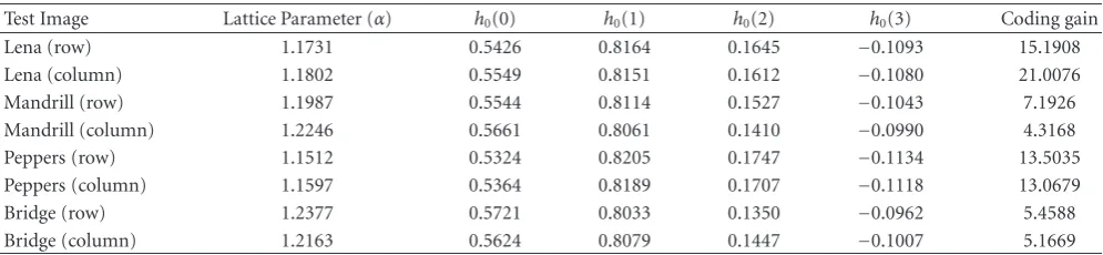
Table2: Lattice parameters of the test images and the corresponding low-pass filter coefficients and coding gains.
Test Image Lattice Parameter (α) h0(0) h0(1) h0(2) h0(3) Coding gain
Lena (row) 1.1731 0.5426 0.8164 0.1645 −0.1093 15.1908
Lena (column) 1.1802 0.5549 0.8151 0.1612 −0.1080 21.0076
Mandrill (row) 1.1987 0.5544 0.8114 0.1527 −0.1043 7.1926
Mandrill (column) 1.2246 0.5661 0.8061 0.1410 −0.0990 4.3168
Peppers (row) 1.1512 0.5324 0.8205 0.1747 −0.1134 13.5035
Peppers (column) 1.1597 0.5364 0.8189 0.1707 −0.1118 13.0679
Bridge (row) 1.2377 0.5721 0.8033 0.1350 −0.0962 5.4588
Bridge (column) 1.2163 0.5624 0.8079 0.1447 −0.1007 5.1669
Table3: Lattice parameters at the maximum coding gains and the corresponding low-pass filter coefficients.
Test Image Lattice Parameter (α) h0(0) h0(1) h0(2) h0(3) Coding Gain
Lena (row) 1.0521 0.4853 0.8359 0.2218 −0.1288 15.7026
Lena (column) 1.0524 0.4855 0.8358 0.2216 −0.1287 21.8264
Mandrill (row) 0.9482 0.4345 0.8470 0.2726 −0.1398 9.4769
Mandrill (column) 1.0359 0.4775 0.8379 0.2296 −0.1308 4.6043
Peppers (row) 1.0371 0.4781 0.8378 0.2290 −0.1307 13.7553
Peppers (column) 1.0372 0.4781 0.8378 0.2290 −0.1307 13.2861
Bridge (row) 1.0505 0.4846 0.8361 0.2225 −0.1290 5.5726
Bridge (column) 1.0547 0.4866 0.8355 0.2205 −0.1284 5.2838
Table4: Daub-2 low-pass filter coefficients.
Coefficient Value
h0(0) 0.4830
h0(1) 0.8365
h0(2) 0.2241
h0(3) −0.1294
the compression capabilities of these QMF filters, the rows and columns of the test images are applied as inputs to the two-stage subband decomposition system given in Figure 1(b)and four sub-signals are obtained. The energies, that is, the variances, of these sub-signals are used to compute the coding gains. Coding gain is given by the following equation [15]:
GTC=
(1/4)4k=1σk2
4
k=1σk2
1/4, (33)
where σk,k = 1, 2, 3, 4 are the variances of the subbands. This expression also corresponds to the arithmetic mean of variances divided by geometric mean of the same variances. This expression measures how much the energy of the input signal is compacted in one of the subbands after the transform. The higher the coding gain, the higher the compression ratios can be obtained after the subband decomposition [15].
The lattice parameters obtained from row- and column-KLT matrices of the test images are given in Table 2 with the corresponding low-pass filter coefficients and the coding gains obtained after the two-stage subband decomposition.
The maximum possible coding gains that could be obtained using the QMF banks are listed in the last column of Table 3 with the lattice parameters and low-pass filter coefficients.
Figure 4shows the graphs of the coding gains computed by (33) and the squared errors, computed by (28), between the row-KLT matrices of the test images and the BWT matrices obtained for each value ofαin the range [0, 2π]. It is seen from the graphs that the lattice parameter angle found by the BWT inversion method is close to the angle at which the maximum coding gain occurs. This observation also provides a motivation for the argument of achieving BWT matrices close to KLT matrices.
In order to make a comparison with a filter bank with the same filter-tap size, the Daub-2 filter was considered. The Daub-2 filter bank can be generated by the lattice parameter
α=π/3 and this parameter is indicated onFigure 4. Daub-2 lattice parameter is very close to the angle of the maximum coding gain for the three of the test images: Lena, Peppers, and Bridge. The Mandrill image contains a lot of high frequencies and therefore Daub-2 is not as successful on Mandrill as the other images. The Daub-2 filter coefficients are given inTable 4. The coding gains obtained by Daub-2 filters are shown inTable 5for each test image. Due to the floating-point precision limits, these coding gains are very close to the maximum coding gains.
Table5: Coding gains obtained by Daub-2 filter bank.
Image Coding Gain
Lena (row) 15.7017
Lena (column) 21.8251
Mandrill (row) 9.0181
Mandrill (column) 4.6032
Peppers (row) 13.7534
Peppers (column) 13.2847
Bridge (row) 5.5726
Bridge (column) 5.2835
decomposed into subbands using the BWT inversion filter banks can be compressed with the compression ratios as good as the compression ratios that can be achieved by the Daub-2 filter bank.
5.3. 8×8 Case. The BWT inversion method can be applied to the 8×8 case by the same way as the 4×4 case. In this case, three lattice parameters,t0,t1, andt2are obtained by the lattice parameterization method. The coefficients of the low-pass QMF filter are then given by the following equations [19]:
t3=π
4−t0−t1−t2,
h0(1)=cos(t3) cos(t2) cos(t1) cos(t0),
h0(2)=cos(t3) cos(t2) cos(t1) sin(t0),
h0(3)= −cos(t3) cos(t2) sin(t1) sin(t0)
−cos(t3) sin(t2) sin(t1) cos(t0)
−sin(t3) sin(t2) cos(t1) cos(t0),
h0(4)=cos(t3) cos(t2) sin(t1) cos(t0)
−cos(t3) sin(t2) sin(t1) sin(t0)
−sin(t3) sin(t2) cos(t1) sin(t0),
h0(5)= −cos(t3) sin(t2) cos(t1) sin(t0)
+ sin(t3) sin(t2) sin(t1) sin(t0)
−sin(t3) cos(t2) sin(t1) cos(t0),
h0(6)=cos(t3) sin(t2) cos(t1) cos(t0)
−sin(t3) sin(t2) sin(t1) cos(t0)
−sin(t3) cos(t2) sin(t1) sin(t0),
h0(7)= −sin(t3) cos(t2) cos(t1) sin(t0),
h0(8)=sin(t3) cos(t2) cos(t1) cos(t0).
(34)
The quadrature mirror high-pass filter pair is computed by ordering the low-pass filter coefficients in the reverse order and changing the signs of the even-ordered coefficients, similar to (15). When this filter bank is used in the three-stage decompositions structure, the BWT matrix is obtained in the following form:
A
= ⎡ ⎢ ⎢ ⎢ ⎢ ⎢ ⎢ ⎢ ⎢ ⎢ ⎢ ⎢ ⎢ ⎢ ⎢ ⎢ ⎢ ⎢ ⎢ ⎢ ⎢ ⎢ ⎢ ⎢ ⎢ ⎢ ⎢ ⎣
1 2√2
1 2√2
1 2√2
1 2√2
1 2√2
1 2√2
1 2√2
1 2√2
A B −C −D −A −B C D
−E −F E F −E −F E F
−C −D −A −B C D A B
1 2√2 −
1 2√2
1 2√2 −
1 2√2
1 2√2 −
1 2√2
1 2√2 −
1 2√2
G −H −I J −G H I −J
−F E F −E −F E F −E
−I J −G H I −J G −H
⎤ ⎥ ⎥ ⎥ ⎥ ⎥ ⎥ ⎥ ⎥ ⎥ ⎥ ⎥ ⎥ ⎥ ⎥ ⎥ ⎥ ⎥ ⎥ ⎥ ⎥ ⎥ ⎥ ⎥ ⎥ ⎥ ⎥ ⎦ ,
(35)
whereA,B,C,D,E,F,G,H,I, andJare some functions of the lattice parameterst0,t1, andt2. All of these coefficients are written in huge expressions in terms of the lattice parameters and it is hard to write down an analytical expression for the optimum lattice parameter. Therefore, only the situation while passing from 4×4 to 8×8 will be examined and the matching the BWT matrix to the KLT matrix will be mentioned.
First of all, the correct column order which matches the BWT and KLT matrices should be discovered, as explained in Section 5.1. To find the correct column order, the sequencies of the rows of the BWT matrix and the lattice parameters by which the maximum coding gain is achieved can be examined.
When the row- and column-KLT matrices of the four test images are examined, it is seen that the second rows of each KLT matrices are sorted in the descending order except the column-KLT of the Mandrill and the row- and column-KLT matrices of the Bridge images. We can conclude from this observation that the KLT matrix distinguishes different features for the Mandrill and Bridge images since they contain more high-frequency components than the other images. As a result, we can select a column order which sorts the second row of the BWT matrix in the descending order.
It is observed that the maximum coding gains are obtained with the BWT matrices whose second row orders are similar, that is, when the columns of the BWT matrices are ordered in the column order 1-8-2-7-3-6-4-5, then the second rows become sorted in the descending order. The only exception for this order is the columns of the Mandrill image (the mentioned column-order for the Mandrill image is 8-1-7-2-6-3-5-4).
α Squar ed er ro r/c o ding ga in
1 2 3 4 5 6
0 0 2 4 6 8 10 12 14 16
α=π/3, daubechies 2
α=1.0521, maximum coding gain
α=1.1731, minimum error
(a) Squar ed er ror/c oding gain 1 2 3 4 5 6 7 8 9 10 α
1 2 3 4 5 6
0
α=π/3, daubechies 2
α=0.9481, maximum coding gain
α=1.1987, minimum error
0 (b) 0 2 4 6 8 10 12 14 Squar ed er ror/c oding gain α
1 2 3 4 5 6
0
α=π/3, daubechies 2
α=1.0371, maximum coding gain
α=1.1512, minimum error
Error Coding gain
(c)
α
1 2 3 4 5
0
α=π/3, daubechies 2
α=1.0505, maximum coding gain
α=1.2136, minimum error
Squar ed er ro r/c o ding gain 1 2 3 4 5 6 7 8 9 0 Error Coding gain (d)
Figure4: Graphs of coding gains and errors for test images: (a) Lena, (b) Mandrill, (c) Peppers, and (d) Bridge.
is obtained: A(ord) = ⎡ ⎢ ⎢ ⎢ ⎢ ⎢ ⎢ ⎢ ⎢ ⎢ ⎢ ⎢ ⎢ ⎢ ⎢ ⎢ ⎢ ⎢ ⎢ ⎢ ⎢ ⎢ ⎢ ⎢ ⎢ ⎢ ⎢ ⎣ 1 2√2
1 2√2
1 2√2
1 2√2
1 2√2
1 2√2
1 2√2
1 2√2
A D B C −C −B −D −A
−E F −F E E −F F −E
−C B −D A −A D −B C
1 2√2 −
1 2√2 −
1 2√2
1 2√2
1 2√2 −
1 2√2 −
1 2√2
1 2√2
G −J −H I −I H J −G
−F −E E F F E −E −F
−I −H J G −G −J H I
⎤ ⎥ ⎥ ⎥ ⎥ ⎥ ⎥ ⎥ ⎥ ⎥ ⎥ ⎥ ⎥ ⎥ ⎥ ⎥ ⎥ ⎥ ⎥ ⎥ ⎥ ⎥ ⎥ ⎥ ⎥ ⎥ ⎥ ⎦ , (36)
By inspecting the sequencies of the rows ofA(ord), it is observed that the sequency of the first row is 0 because all elements are the same. The coefficientsA,D,B, andCin the second row are all positive since the second row is sorted in the descending order, as explained above. So, the sequency for the second row is 1/2. IfEandFhave opposite signs, then the sequency of the third row becomes 2/2. The fourth row has the same coefficients as the second row, so the sequency of the fourth row is 7/2. The elements in the fifth row are fixed and they make the sequency of the fifth row as 4/2. If
Table6: Channel variances.
Test Image Method Ch.1 Ch.2 Ch.3 Ch.4
Lena (row)
BWT Inversion 0.1576 0.0022 0.0003 0.0005
Daub-2 0.1576 0.0022 0.0002 0.0005
Max. Coding Gain 0.1576 0.0022 0.0002 0.0005
Lena (col.)
BWT Inversion 0.1579 0.0015 0.0002 0.0003
Daub-2 0.1579 0.0015 0.0001 0.0003
Max. Coding Gain 0.1579 0.0015 0.0001 0.0003
Mandrill (row)
BWT Inversion 0.0890 0.0076 0.0003 0.0007
Daub-2 0.0892 0.0078 0.0002 0.0004
Max. Coding Gain 0.0892 0.0080 0.0002 0.0003
Mandrill (col.)
BWT Inversion 0.0867 0.0084 0.0005 0.0029
Daub-2 0.0868 0.0085 0.0004 0.0028
Max. Coding Gain 0.0868 0.0085 0.0004 0.0028
Peppers (row)
BWT Inversion 0.1738 0.0020 0.0005 0.0006
Daub-2 0.1739 0.0020 0.0005 0.0006
Max. Coding Gain 0.1739 0.0020 0.0005 0.0006
Peppers (col.)
BWT Inversion 0.1748 0.0019 0.0006 0.0008
Daub-2 0.1749 0.0018 0.0005 0.0007
Max. Coding Gain 0.1749 0.0018 0.0005 0.0007
Bridge (row)
BWT Inversion 0.1698 0.0062 0.0015 0.0029
Daub-2 0.1701 0.0061 0.0015 0.0029
Max. Coding Gain 0.1702 0.0061 0.0015 0.0029
Bridge (col.)
BWT Inversion 0.1674 0.0081 0.0012 0.0034
Daub-2 0.1676 0.0082 0.0012 0.0033
Max. Coding Gain 0.1676 0.0082 0.0012 0.0022
Table7: Lattice parameters obtained by BWT inversion, squared errors, coding gains, and Daub-4 coding gains for the test images.
Image t0 t1 t2 Error Coding gain Daub-4 Coding Gain
Lena (Row) 0.2050 1.7578 2.3681 1.5799 29.0332 28.1603
Lena (Column) 0.1815 1.7548 2.3792 1.9057 42.3720 40.9648
Mandrill (Row) 0.1076 1.7306 2.4510 6.6210 19.4572 11.1199
Mandrill (Column) 0.2639 1.7654 2.3397 0.3251 10.8046 8.7974
Peppers (Row) 0.1145 1.7522 2.4255 1.6738 21.7710 21.0646
Peppers (Column) 3.0985 1.7363 2.5385 1.0668 20.2952 20.0228
Bridge (Row) 3.2223 1.7654 2.4497 1.2905 7.5605 7.3931
Bridge (Column) 1.7719 0.8179 2.7880 0.8227 7.2874 7.1124
Consequently, we have ordered the columns according to the second row and the rows according to the sequencies of the rows. After this, the signs of the rows are further altered to match the column sequencies, too.
Interchanging the rows and columns of the BWT matrix corresponds to interchanging the input signals which are used to generate the BWT matrix and it does not affect the orthogonality of the BWT matrix, as explained inSection 5.1. Changing the sign of a row of the BWT matrix corresponds to changing the sign of a 1 in the input vectors, and again, it does not affect the orthogonality of the BWT matrix. From the KLT point of view, changing row order, column order,
or signs corresponds to bring a specific feature forth or send it back. Notice that, since KLT also internally orders the eigenvectors of the autocorrelation matrix according to the eigenvalues, the above described operation is reasonable.
Table8: The channel variances and percentages obtained by the BWT Inversion and the Daub-4 filter banks.
Test Image Method Ch.1 Ch.2 Ch.3 Ch.4 Ch.5 Ch.6 Ch.7 Ch.8
Lena (Rows)
BWT Inversion 0.3077 0.0085 0.0009 0.0027 0.0001 0.0001 0.0005 0.0003
(95.93%) (2.64%) (0.27%) (0.84%) (0.04%) (0.05%) (0.16%) (0.08%)
Daub-4 0.3143 0.0089 0.0009 0.0028 0.0001 0.0002 0.0005 0.0003
(95.83%) (2.72%) (0.27%) (0.84%) (0.03%) (0.05%) (0.17%) (0.09%)
Lena (Columns)
BWT Inversion 0.3049 0.0057 0.0006 0.0019 0.0001 0.0001 0.0003 0.0002
(97.21%) (1.81%) (0.18%) (0.60%) (0.02%) (0.04%) (0.10%) (0.05%)
Daub-4 0.3114 0.0060 0.0006 0.0019 0.0001 0.0001 0.0003 0.0002
(97.12%) (1.89%) (0.18%) (0.60%) (0.02%) (0.04%) (0.10%) (0.06%)
Mandrill (Rows)
BWT Inversion 0.1598 0.0187 0.0045 0.0095 0.0000 0.0000 0.0005 0.0001
(82.74%) (9.67%) (2.33%) (4.92%) (0.01%) (0.02%) (0.24%) (0.07%)
Daub-4 0.1574 0.0189 0.0038 0.0092 0.0000 0.0001 0.0014 0.0006
(82.19%) (9.88%) (1.97%) (4.81%) (0.02%) (0.08%) (0.72%) (0.33%)
Mandrill (Columns)
BWT Inversion 0.1595 0.0178 0.0050 0.0121 0.0000 0.0001 0.0031 0.0007
(80.45%) (8.99%) (2.50%) (6.12%) (0.01%) (0.05%) (1.56%) (0.33%)
Daub-4 0.1610 0.0182 0.0062 0.0125 0.0001 0.0001 0.0023 0.0007
(80.06%) (9.06%) (3.07%) (6.21%) (0.04%) (0.07%) (1.13%) (0.37%)
Peppers (Rows)
BWT Inversion 0.3390 0.0081 0.0008 0.0022 0.0004 0.0005 0.0006 0.0004
(96.29%) (2.29%) (0.24%) (0.62%) (0.12%) (0.13%) (0.18%) (0.12%)
Daub-4 0.3363 0.0086 0.0009 0.0023 0.0005 0.0004 0.0006 0.0005
(96.06%) (2.45%) (0.26%) (0.66%) (0.13%) (0.12%) (0.17%) (0.13%)
Peppers (Columns)
BWT Inversion 0.3450 0.0064 0.0010 0.0022 0.0005 0.0005 0.0009 0.0005
(96.64%) (1.79%) (0.29%) (0.62%) (0.13%) (0.14%) (0.24%) (0.15%)
Daub-4 0.3463 0.0071 0.0011 0.0024 0.0005 0.0005 0.0008 0.0006
(96.43%) (1.97%) (0.29%) (0.66%) (0.14%) (0.14%) (0.21%) (0.16%)
Bridge (Rows)
BWT Inversion 0.3209 0.0150 0.0041 0.0074 0.0011 0.0014 0.0033 0.0018
(90.37%) (4.22%) (1.16%) (2.09%) (0.31%) (0.40%) (0.92%) (0.52%)
Daub-4 0.3189 0.0155 0.0042 0.0077 0.0012 0.0014 0.0032 0.0020
(90.08%) (4.37%) (1.20%) (2.18%) (0.34%) (0.39%) (0.89%) (0.55%)
Bridge (Columns)
BWT Inversion 0.3103 0.0208 0.0055 0.0099 0.0009 0.0010 0.0033 0.0018
(87.77%) (5.88%) (1.56%) (2.81%) (0.25%) (0.28%) (0.95%) (0.51%)
Daub-4 0.3036 0.0211 0.0050 0.0101 0.0008 0.0011 0.0033 0.0019
(87.51%) (6.08%) (1.44%) (2.90%) (0.24%) (0.33%) (0.95%) (0.56%)
are computed for all local minima. The local minima which give the maximum coding gain for each of the test images are listed inTable 7. The results show that better coding gains are obtained by the proposed method as compared to the Daub-4 filter bank, which has the same filter-tap size.
It is observed that the maximum coding gain occurs at one of the local parametric minima, but that point is not necessarily the global minimum. This situation can be explained by the characteristics of the KLT matrix. The features that make the coding gain maximum may require some extra constraints to reach to the global optimum.
The channel variances obtained by the BWT inversion and the Daub-4 filter banks are listed inTable 8. The channel
variances show that the BWT Inversion method collects most of the information in the first subband.
6. Conclusion
the previous works, the parameterization is constructed for 2-channel dyadic filter banks and their extensions. Due to the limitation in degree of freedom (i.e., single parameter for 4 channel decomposition and 3 parameters for 8 channel decomposition), exact matching of the produced BWT and real KLT is almost impossible. In that case, it is proposed that the QMF structure, which produces a BWT matrix that is as close to KLT as possible (in RMSE sense), should produce a good performance. The validity of this argument is verified over experiments of compaction ratio evaluation over test images.
The work is explained in two parts. In the first part, an analytical method to construct the QMF filter bank of size 4×4 is developed. Developing an analytical method for the size 8×8 is difficult because the number of terms in the equations increases exponentially and the solutions produce overly complicated and long expressions. Thus, the 8×8 case is considered in the second part and numerical computation method for matching KLT and BWT is adopted.
The coding gains obtained by the BWT inversion and the equal-sized filter banks in the Daubechies family are compared. In the 4×4 case, the Daub-2 filter bank generates slightly better coding gains, but BWT inversion method separates the signal into subbands whose variances are close to the variances obtained by the Daub-2 filter bank. On the other hand, it must be noted that the parameterization of the 4×4 case is really low (just one parameter), and any optimization attempt has very limited effect. In the 8×8 case, however, greater coding gains are obtained for all of the test images. Again, most of the signal energies are gathered in the first subband. So, the BWT inversion method gives better result than the Daub-4 filter bank. The reason to this improvement can be explained due to better parameter degree of freedom (three parameters) for the exploitation of the KLT similarity. Consequently more features of the KLT matrix are revealed in the 8×8 case. It is reasonable to assume that this property could provide better performance for higher orders of two. However, due to the complexity of the analytical expressions in higher orders, more emphasis is expected to be paid on numerical approximations of the described BWT-KLT matching idea in QMF filter bank design.
References
[1] A. K. Jain,Fundamentals of Digital Image Processing, Prentice-Hall, Englewood Cliffs, NJ, USA, 1989.
[2] J. W. Woods,Subband Image Coding, Kluwer, Norwood, Mass, USA, 1991.
[3] I. Daubechies, “Orthonormal bases of compactly supported wavelets,”Communications on Pure & Applied Mathematics, vol. 41, no. 7, pp. 909–996, 1988.
[4] S. G. Mallat, “Theory for multiresolution signal decomposi-tion: the wavelet representation,”IEEE Transactions on Pattern Analysis and Machine Intelligence, vol. 11, no. 7, pp. 674–693, 1989.
[5] E. Cetin and O. N. Gerek, “Block wavelet transform for image coding,”IEEE Transactions on Circuits and Systems for Video Technology, vol. 3, no. 6, pp. 433–435, 1993.
[6] S. Akkarakaran and P. P. Vaidyanathan, “Filterbank optimiza-tion with convex objectives and the optimality of principal component forms,”IEEE Transactions on Signal Processing, vol. 49, no. 1, pp. 100–114, 2001.
[7] M. Dogan and O. N. Gerek, “Subband decomposition filter bank design from the inverse block wavelet transform using LMS optimization,” inProceedings of International Workshop III: Mini Symposium on Applications of Wavelets to Real World Problems (IWW ’08), Istanbul, Turkey, 2008.
[8] M. Dogan and O. N. Gerek, “Performance analysis of QMF filters obtained by the inverse block wavelet transform,” in Proceedings of International Conference on Electronics and Computer (IKECCO ’08), Bishkek, Kyrgyzstan, 2008. [9] M. Dogan and O. N. Gerek, “On the orthogonality of block
wavelet transforms,” inProceedings of the 14th IEEE Signal Processing and Communications Applications Conference (SIU ’06), Antalya, Turkey, 2006.
[10] H. Hotelling, “Analysis of a complex of statistical variables into principal components,”Journal of Educational Psychology, vol. 24, no. 7, pp. 498–520, 1933.
[11] K. Karhunen, “ ¨Uber Lineare Methoden in der Wahrschein-lichkeitsrechnung,”Annales Academiae Fennicae, Series A, vol. 37, pp. 1–79, 1947.
[12] M. Lo´eve, “Fonctions Al´eatoires de Seconde Ordre,” in Processus Stochastiques et Mouvement Brownien, P. Levy, Ed., Hermann, 1948.
[13] H. P. Kramer and M. V. Mathews, “A linear encoding for transmitting a set of correlated signals,”IRE Transactions on Information Theory, vol. 2, pp. 41–46, 1956.
[14] J. Y. Huang and P. M. Schultheiss, “Block quantization of correlated Gaussian random variables,”IEEE Transactions on Communication Systems, vol. 11, pp. 289–296, 1963.
[15] K. Sayood,Introduction to Data Compression, Morgan Kauff -mann, San Francisco, Calif, USA, 3rd edition, 2006.
[16] P. P. Vaidyanathan and P. Q. Hoang, “Lattice structures for optimal design and robust implementation of two-channel perfect-reconstruction QMF banks,” IEEE Transactions on Acoustics, Speech, and Signal Processing, vol. 36, no. 1, pp. 81– 94, 1988.
[17] J. A. Saghri, A. J. Tescher, and J. T. Reagan, “Terrain adaptive transform coding of multispectral data,” in Proceedings of International Conference on Geosciences and Remote Sensing (IGARSS ’94), pp. 313–316, 1994.
[18] P. P. Vaidyanathan,Multirate Systems and Filter Banks, Prentice Hall, Upper Saddle River, NJ, USA, 1993.
[19] I. W. Selesnick, “Maple and parameterization of orthogonal wavelet bases,” Tech. Rep., ECE Dept. and Computational Mathematics Laboratory, Rice University, Houston, Tex, USA, 1997.