Iterative Approximation of Empirical Grey-Level Distributions for Precise Segmentation of Multimodal Images

Iterative Approximation of Empirical Grey-Level

Distributions for Precise Segmentation

of Multimodal Images

Ayman El-Baz

CVIP Laboratory, Department of Electrical and Computer Engineering, University of Louisville, Louisville, KY 40292, USA Email:[email protected]

Aly A. Farag

CVIP Laboratory, Department of Electrical and Computer Engineering, University of Louisville, Louisville, KY 40292, USA Email:[email protected]

Georgy Gimel’farb

Centre for Image Technology and Robotics (CITR), Department of Computer Science, University of Auckland, Tamaki Campus, Auckland 1000, New Zealand

Email:[email protected]

Received 29 December 2003; Revised 5 December 2004

A new algorithm for segmenting a multimodal grey-scale image is proposed. The image is described as a sample of a joint Gibbs random field of region labels and grey levels. To initialize the model, a mixed multimodal empirical grey-level distribution is approximated with linear combinations of Gaussians, one combination per region. Bayesian decisions involving expectation max-imization and genetic optmax-imization techniques are used to sequentially estimate and refine parameters of the model, including the number of Gaussians for each region. The final estimates are more accurate than with conventional normal mixture mod-els and result in more adequate region borders in the image. Experiments show that the proposed technique segments complex

multimodal medical images of different types more accurately than several other known algorithms.

Keywords and phrases:density estimation, image segmentation, expectation maximization.

1. INTRODUCTION

A large number of image segmentation methods based on estimating marginal probability densities of signals and sepa-rating their dominant modes have been developed and tested for the last three decades (see [1,2,3,4,5] to cite a few). However many important applications such as medical im-age analysis or industrial vision still encounter difficulties in separating practically meaningful continuous or disjoint objects, even when signal densities are distinct to the point where their mixture becomes strongly multimodal. The ba-sic issue is the accuracy of region borders, which are usually essential for correct interpretation of the objects. Typically, the fine separation of the signal modes to specify the region borders is obtained by intersecting tails of the signal distri-butions for the adjacent objects. Therefore, it is the tails that have to be precisely estimated in order to separate, for exam-ple, a darker object from a brighter background. One of the practical problems that inspired our approach is to accurately

detect lungs in a spiral CT chest slice so that their borders closely match those outlined by a radiologist.

than a conventional normal mixture with only the positive components. Then a mixed empirical signal distribution over the image is approximated with a mixture of several lin-ear combinations of Gaussians. Such a lower-level segmen-tation on the basis of the estimated probability densities is refined further at the higher level using the Bayesian max-imum a posteriori (MAP) estimation of the segmentation map based on the joint Gibbs model of the maps and im-ages.

We propose a new sequential EM-based algorithm that closely approximates a given multimodal empirical probabil-ity distribution of signals by estimating parameters of the lin-ear combination of Gaussians for each region. Below for sim-plicity, we restrict our consideration to only a bimodal signal density describing a dark object and its bright background. But the extension of the proposed segmentation scheme onto the multimodal case is straightforward. In the bimodal case, the empirical mixed density is split first into two dominant positive Gaussians and a set of secondary alternating Gaus-sians. These latter describe deviations of the empirical distri-bution from the dominant components. The number of the dominant modes (i.e., the number of different types of re-gions to detect) is assumed to be known, but the number of the secondary terms is found on the basis of the approxima-tion error.

The parameters of both the dominant and secondary terms are sequentially estimated using the EM-algorithm [17, 18, 19,20,21], or more specific, its early variant for the normal mixtures [22] (see also [21]). To initially segment the image, the approximated mixed density is divided further into two linear combinations of Gaussians (for the darker object and the brighter background, resp.) which yield the minimum classification error on the intersecting tails of the distributions.

At the higher level, the label intra- and interregion co-occurrences are specified by an auto-binomial Gibbs model with the nearest 8-neighborhood [11,13]. The region map after an initial low-level classification is refined iteratively by repeating the following steps: (i) updating the higher-level map, given the low-level image model, and (ii) updating this latter, given the region map.

The paper is organized as follows.Section 2introduces the Gibbs image model and describes the low-level and high-level stages of the proposed segmentation algorithm. Section 3describes experiments with different types of med-ical images to show that the proposed technique produces region borders close to the “ground truth” given by the experts—radiologists—and is more accurate than several other segmentation algorithms.

2. TWO-LEVEL GIBBS IMAGE MODEL

LetR = {(x,y) : 1 ≤x ≤X, 1≤ y≤ Y}be a finite grid supporting imagesg :R→Qand their region mapsl:R→

K. HereQ= {0,. . ., 255}andK= {1,. . .,K}are the sets of grey levelsq ∈Qand region labelsk∈K, respectively (for the bimodal case,K= {1, 2}).

The two-level Gibbs image model is specified by a joint probability distribution P(g,l) = P(g|l)P(l), where P(l) is a prior higher-level Gibbs distribution of maps and P(g|l) is a lower-level conditional distribution of images, given the map. Both the distributions are strictly positive. The MAP estimatel∗ =arg maxlL(g,l) of the map, given the imageg,

maximizes the joint log-likelihood function:

L(g,l)=logP(g|l) + logP(l). (1)

To make the choice computationally feasible, a local maxi-mum of the log likelihood of (1) is usually searched for it-eratively by estimating or reestimating first the lower-level model and then using it to update the higher-level one. The process terminates when parameters of the current and per-vious estimated models become equal to a value within a given accuracy range [7,9,10,16].

Such an iterative maximization using the lower-level model in an explicit form and the higher-level model with numerically approximated components having no closed-form representation is implemented below.

2.1. Low-level density model

To most accurately specify the lower-level model, we approx-imate the marginal grey-level probability density function in each regionk =1, 2,. . .,Kwith a linear combination ofCk

Gaussians [14,15]: for eachq∈Q,

p(q|k)=

Ck

i=1

wk,iϕ

q|θk,i

;

_∞

−∞p(q|k)dq=1. (2)

Here, in contrast to the more conventional normal mixture models, the weights wk,i may be both positive and

nega-tive and have only one obvious restriction in line with (2):

Ck

i=1wk,i =1. The weights now are not prior probabilities,

and the combination in (2) is simply an approximation of the probability density function depending on parameters wk,i,

θk,idenoting the weight and the mean and variance of each

component, respectively.

(C =C1+C2+· · ·+CK if all the valuesθk,idiffer for both

distributions):

p(q)=

C

c=1

wcϕ

q|θc

, (3)

where all the mixed elements do not relate to the regions and thus have only one subscriptc. In principle, all the parame-tersw= {wc;c=1,. . .,C}andθ= {θc:c=1,. . .,C}, given

the number of the componentsC, can be sequentially found using an EM algorithm modified to account for the alternat-ing signs of the weights. This modification will be consid-ered elsewhere. Here an alternative EM-based approach for describing the multimodal density of (3) is used. The EM al-gorithm is quite natural in this MAP framework because it maximizes the first term, logP(g|l), in the log likelihood of (1).

We assume that the number of objects (types of regions) to be separated, or what is the same, the number of the dom-inant modes, is known for all the images to be segmented. For simplicity, let the empirical distribution have two sepa-rate dominant modes that represent the object and the back-ground, respectively, and each can be roughly approximated with a single Gaussian. Deviations of the empirical distri-bution from the two-component dominant Gaussian mix-ture are described by other components of (3). Therefore there are two dominant positive weights, say,w1andw2, such

thatw1+w2=1, and the “subordinate” weights with much

smaller absolute values such thatw3+· · ·+wC=0.

To estimate parameters of this latter model (both the weight and the parameters of each individual Gaussian) and get the initial region map, we propose the following sequen-tial algorithm (with obvious modifications, it can be used also to approximate either a unimodal empirical distribution or a distribution with three and more dominant modes).

(1) Form the empirical mixed density function from the relative frequencies f(q|g) of grey levels in all the pixels (x,y)∈ R, its integral over the−∞ ≤ q ≤ ∞range being equal to the sum of all the frequencies:

F(g)=

f(q|g) :q∈Q;

q∈Q

f(q|g)=1

. (4)

(2) Use the conventional EM-algorithm to approximate F(g) with a dominant mixtureP2of two Gaussians:

p2(q)=w1ϕ

q|θ1

+w2ϕ

q|θ2

. (5)

(3) Find the deviation∆ofF(g) fromP2:

∆=δ(q)= f(q|g)−p2(q) :q∈Q (6)

and split it into the positive and negative parts:

∆p=

δp(q) :q∈Q , ∆n=

δn(q) :q∈Q

(7)

such that

δ(q)=δp(q)−δn(q);

δp(q)=   

δ(q) ifδ(q)>0, 0 otherwise;

δn(q)=   

0 ifδ(q)<0, −δ(q) otherwise.

(8)

(4) Compute the scaling factor for the deviations:

s=

_∞

−∞δp(q)dq≡

_∞

−∞δn(q)dq. (9)

(5) Ifs≤ τ (a given accuracy threshold), terminate the process and output the modelP=P2.

(6) Otherwise, consider the scaled-up absolute deviation

∆abs=1/2s(∆p+∆n) as an “empirical density” and use

itera-tively the EM-algorithm to find the numberCsecof Gaussians

such that their mixture approximates best the scaled-up ab-solute deviation; this search for the number of the secondary components is detailed below.

(7) Scale down the obtained mixture modelP3,...,C, that

is, scale down its weights:wi→s·wc;c=3,. . .,C =Csec+

2, and change the signs of the individual weights in accord with the corresponding deviations to obtain the alternating scaled-down modelsP3,...,C, where each Gaussian is assigned

with the sign of the deviation closest to the mean value for that component.

(8) Center the model P3,...,C in order to guarantee zero

sum of its weights and output the modelP=P2+sP3,...,C.

Instead of the last three steps, the scaled-up absolute de-viations (1/s)∆pand (1/s)∆ncan be separately approximated

with the two normal mixtures having Cp and Cn

compo-nents, respectively. Then the scaled-down submodelsPCpand PCn are added to and subtracted from the modelP2, respec-tively, in order to output the desired modelP. Both variants have produced almost the same final models in our experi-ments. While the latter variant is more theoretically justified, the former one is twice as fast.

Since the EM algorithm converges to a local maximum of the likelihood function, it may be repeated several times with different initial parameter values as to choose the modelP yielding the best approximation. In principle, the process can be continued iteratively in order to approximate more and more closely the residual absolute deviations betweenF(g) andP. But because each Gaussian in the modelPimpacts all the density values p(q), the iterations should be terminated when the approximation quality begins to decrease.

We specify the approximation quality by the Kullback-Leibler divergence between the empirical and estimated den-sities in the pointsq∈Q:

DF(g),P=

q∈Q

f(q|g) log

f(q|g) p(q)

The above divergence is zero if f(q|g) = p(q) for allq ∈

Q, that is, for the exact approximation, otherwise it specifies how far is the log likelihood of the current model from its maximum value for the exact one. Letεqdenote the relative

approximation error such thatp(q)=(1 +εq)f(q|g). Then

DF(g),P= −

q∈Q

f(q|g) log1 +εq

≈1 2

q∈Q

f(q|g)ε2q

(11)

so that 0 ≤ D(F(g),P) ≤ (1/2) maxq∈Qε2q. The sequential

process has to be terminated when the divergence of (10) is closest to zero or, what is almost the same, when the weighted sum of the squared relative errors has the minimum value.

The search for a numbercof the Gaussians in the model is based on the integral absolute errorE(∆abs,P3,...,C) between

the scaled-up absolute deviation ∆abs acting as the density

function and its mixture modelP3,...,C. The numbercof the

components is increasing sequentially by unit step until the errorE(·) begins to increase. Once again, due to the multi-ple local maxima, the search has to be repeated several times with different initial parameter values as to select the best ap-proximation.

Now the final mixed modelPhas to be split into the two parts by relating the subordinate components to either the object or the background so as to minimize the expected er-ror of classification. Let the two dominant Gaussians with the meansµ1 andµ2, 0 < µ1 < µ2 < qmax, correspond to

the background and the object, respectively. Then the subor-dinate components having the mean values greater thanµ2

and lesser thanµ1belong to the object and the background,

respectively. Other components having the means in the in-terval [µ1,µ2] are compared to a thresholdtin that interval

as to get the minimum classification error

e(t)=

t

−∞p(q|2)dq+

_∞

t p(q|1)dq. (12)

2.2. High-level region model

We describe the region maps as samples of a simple auto-binomial Gibbs model [13] such that a region labell(x,y) in the pixel (x,y)∈Rdepends on only its four nearest neigh-borsl(x+ξi,y+ηi); (ξi,ηi)∈N= {[1, 0]; [1, 1]; [0, 1]; [1, 1]};

i=1,. . ., 4. The model is specified with the Gibbs probability distribution:

P(l)= 1 Zexp

U1(l) + 4

i=1

U2,i(l)

, (13)

where Z is a normalizing factor (the partition function) and U1(l) and U2,i(l) denote partial energies of pixelwise

and pairwise interactions of region labels. The energies are the sums of Gibbs potentials {V1(k|α) : k ∈ K} and

{V2,i(j,k|λi) : (j,k) ∈K×K}depending, respectively, on

the labelsk=l(x,y) in the individual pixels and on the label

cooccurrences (j=l(x,y),k=l(x+ξi,y+ηi)), (ξi,ηi)∈N,

in the pairs of similarly oriented neighbors:

U1(l)=

(x,y)∈R V1

l(x,y),

U2,i(l)=

(x,y)∈R V2,i

l(x,y),lx+ξi,y+ηi

. (14)

Each partial energy can be represented in terms of the po-tentials and relative frequency distributions of the labels Fmap(l) = {f(k|l) : k ∈ K} and their cooccurrences

Fi,map(l)= {f(j,k|l) : (j,k)∈K×K}over the region mapl.

These distributions are sufficient statistics of the model and allow for obtaining rough analytical first approximations of the potentials. The derivation scheme in [11] modified to better fit our model results in the following first approxima-tions of the initial potential values:

V1(k)= −logf(k|l),

V2,i(j,k)=γ

fi(j,k|l)−f(j|l)·f(k|l)

. (15)

The scaling factorγcan be also computed using the distribu-tionsFmap(l) andFi,map(l),i=1,. . ., 4.

Under the assumed continuity of and symmetric rela-tionships between the two regions, all the potentials are bi-valued:

V1(k)=α·k; V2,i(j,k)=   

λi, j=k,

−λi, j=k,

(16)

withα≥0 andλi>0,i=1,. . ., 4.

To find the region map which maximizes the likelihood in (1), the potential estimates are refined using the genetic algorithm (GA) [23]. Because the partition functionZis un-known, it is approximated as proposed in [6]:

Z≈

(x,y)∈R

k∈K exp

V1(k) + 4

i=1

j∈K

V2,i(k,j)

. (17)

To implement the GA optimization, the parametersαandλi,

i = 1,. . ., 4, in (16) are coded into a GA 20-bit “chromo-some” using four bits per value. While the approximate log likelihood of (1) continues to increase, the following steps are repeated iteratively.

(1) Form a randomized population ofN =30 chromo-somes from the top-ranked chromochromo-somes for the previous iteration.

(2) Refine the initial region map using the Metropolis stochastic relaxation [13] with the potentials coded in each chromosome.

(3) Compute the log likelihood value for each chromo-some using the refined map.

2 4 6 8 10 12 14 16 Iteration

−5.4

−5.2

−5

−4.8

−4.6

−4.4

−4.2

Lik

elihood

function

L

(

g,

l

)

Figure1: Convergence of the proposed algorithm (for the

experi-ment inSection 3, seeFigure 2).

Figure2: Typical slice from a chest spiral CT scan.

Iterative refinement:refine the initial map by repeating it-eratively the following two steps:

(1) estimate the higher-level model which gives the maxi-mum increase of the approximate log likelihood of the current region map, given the lower-level image model; (2) recollect the empirical grey-level densities for the cur-rent regions, reapproximate these densities, and update the map using the pixelwise Bayesian classification.

Because at each step the approximate log-likelihood is greater than or equal to its previous value, the proposed algorithm converges to a locally optimum solution. Typical changes of the log-likelihood values in (1) at each iteration of the pro-posed algorithm are shown inFigure 1.

3. EXPERIMENTAL RESULTS

To assess robustness and computational performance, the proposed segmentation technique has been tested on three different medical imaging modalities. The images include axial human chest slices obtained by spiral-scan low-dose computer tomography (LDCT), axial human head slices ob-tained by time-of-flight magnetic resonance angiography (TOF-MRA), and axial human head slices obtained by magnetic resonance imaging (MRI). The two latter types were acquired with the Picker 1.5T Edge MRI scanner.

f(q) p2(q)

0 50 100 150 200 250

q 0

0.005 0.01 0.015

Densit

y

Figure3: Empirical densityF(g)=(f(q) :q∈Q) versus the

dom-inant mixtureP2=(p2(q) :q∈Q).

Table1: Initial (the upper row) and final (the bottom row) param-eter estimates for the dominant Gaussians.

w1 µ1 σ12 w2 µ2 σ22

0.219 36.2 210.6 0.781 166.4 315.9

0.242 39.9 225.7 0.758 170.8 303.6

The TOF-MRA 512×512 and MRI 256×256 slices were 1 mm thick. The 8 mm thick LDCT slices were reconstructed every 4 mm with the scanning pitch of 1.5 mm.

In all the cases, the number of classes (i.e., domi-nant modes in the model) is specified by the user, and all other parameters are estimated by the proposed techniques. Section 3.1discusses experiments with bimodal LDCT im-ages. Experiments with three-modal MRA images and four-modal MRI images are described in Sections3.2and3.3, re-spectively.

3.1. Lungs segmentation in LDCT images

We applied the proposed algorithm to a medical screening problem of separating lung tissues from the surrounding anatomical structures (e.g., chest, ribs, liver) in computer to-mography (CT) images. The segmentation assumes that each CT slice has only two regions: the darker one (the lungs) and their brighter background. Because some lung tissues such as arteries, veins, bronchi, and bronchioles have grey levels close to those of the chest, the segmentation based on only the grey levels may lose some of these tissues. To obtain more accurate segmentation, our model accounts also for spatial relationships between the pixels.

Error betweenf(q) andp2(q)

Absolute error betweenf(q) andp2(q)

0 50 100 150 200 250

q

−2

−1

0 1 2 3

×10−3

De

vi

ation

Figure4: Deviations∆(q)= f(q)−p2(q) and the absolute

devia-tions|∆(q)|between the densities inFigure 3.

2 4 6 8 10

Number of components 0.15

0.2 0.25 0.3 0.35 0.4 0.45 0.5

Er

ro

r

Figure5: Error function (E(∆abs,P3,...,C)) versus the numberCof

the subordinate Gaussians approximating the scaled absolute

devi-ation inFigure 4.

0.09 between these two distributions indicates a large mis-match.Figure 4shows the scaled deviation of the dominant mixture from the empirical density. Our estimation of the number of components giving the minimum approximation error returns the ten Gaussians shown inFigure 5.Figure 6 presents the final result of this approximation.

Figure 7shows the estimated density after the subordi-nate linear combination of Gaussians is added to the domi-nant mixture according to the deviation signs. The Levy dis-tance between the empirical and final estimated distributions is now much smaller (0.02) than before (0.09).

Figure 8 shows the 12 components of the model. The Bayesian pixelwise classification is repeated for different partitions of the ten subordinate components. The minimum

0 50 100 150 200 250

q 0

0.5 1 1.5 2 2.×5

10−3

Densit

y

Figure6: Subordinate mixture estimated for the absolute deviation inFigure 4.

0 50 100 150 200 250

q 0

0.005 0.01 0.015

Densit

y

Figure 7: Empirical and estimated densities for the CT slice in

Figure 2(the linear combination of 12 Gaussians).

0 50 100 150 200 250

q

−2

0 2 4 6 8 10 12 14×

10−3

L

C

G

components

p(q|1) p(q|2)

t=108

0 50 100 150 200 250

q 0

0.005 0.01 0.015

Densit

y

Figure 9: Densities estimated for the lung and chest tissues in

Figure 2(the minimum error 0.0045 for the thresholdt=108).

f(q) p2(q)

0 50 100 150 200 250

q 0

0.005 0.01 0.015

Densit

y

Figure10: Approximation of the signal distribution for the CT slice inFigure 2by the conventional mixture of 12 Gaussians.

classification error of 0.0045 on the intersecting distribu-tion tails is obtained for the threshold t = 108 when the components 1–3 and 4–10 correspond to the first class (the lung tissues) and the second class (the chest tissues), respectively (see the estimates for each class in Figure 9).

To highlight advantages of using the linear combination of Gaussians, the same empirical density was approximated with a conventional mixture of 12 Gaussians. The results are shown in Figures 10 and11. The classification error is al-most three times higher (0.013) because one of the compo-nents combines the former tails of both classes and cannot

p(q|1) p(q|2)

t=88

0 50 100 150 200 250

q 0

0.005 0.01 0.015

Densit

y

Figure11: Densities for the lung and chest tissues inFigure 2

esti-mated with the mixture of 12 Gaussians (the minimum error 0.013

for the thresholdt=88).

Table2: The initial and final potentials for the map model for the

LDCT image inFigure 2.

Parameters α λ1 λ2 λ3 λ4

Initial 1 0.81 0.71 0.49 0.51

Final 1 0.89 0.80 0.78 0.69

be related to only the object or the background. Therefore it comes as no surprise that our segmentation algorithm pro-duces more accurate lung borders.

(a) (b)

(c) (d)

(e) (f)

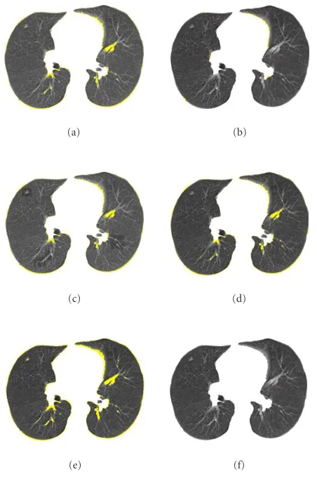
Figure 12: (a) Initial lower-level segmentation; (b) final lung regions (the error of 0.89%); (c) lung regions obtained with the randomly chosen higher-level parameters (the error of 1.86%); (d)

segmentation by the MRS algorithm with the potential values 0.3

and three levels of resolution (the error of 2.3%); (e)

segmenta-tion by the ICM algorithm with the potential values 0.3 (the error

of 2.9%); and (f) lung regions segmented by a radiologist. The

er-rors with respect to this ground truth are highlighted by the yellow color.

Figure 13compares our results to those obtained using the iterative thresholding proposed by Hu and Hoffman [25]. In contrast to their method, our segmentation does not lose ab-normal lung tissues.

But the ground truth given by the radiologist may con-tain by itself errors due to hand positioning instabilities dur-ing the manual segmentation. In order to better measure the accuracy of our approach, we have created a phantom with the same grey-level distribution as the above CT slices. The phantom, its ground truth, and our segmentation are shown in Figure 14. The error 0.091% between the found regions and the ground truth confirms the high accuracy of the pro-posed approach.

The above experiments as well as additional experiments with 120 different bimodal LDCT slices have shown that our

(a)

The error: 0.98% The error: 1.09% (b)

The error: 3.01% The error: 13.1% (c)

(d)

Figure 13: (a) Original CT slices; (b) our lung regions (the seg-mentation errors are only around the outer edge); (c) segseg-mentation

by the method in [25]; and (d) regions given by a radiologist. The

errors are highlighted by the yellow color.

(a) (b) (c)

Figure14: (a) Generated phantom; (b) ground-truth image (black lung and grey chest regions); (c) our segmentation (the error of 0.091% around the outer edge is highlighted by the yellow color).

Table3: Accuracy and time performance of our segmentation in

comparison to the three conventional algorithms (IT [25], MRS [7],

and ICM [6]).

Characteristics Segmentation algorithm

Ours IT MRS ICM

Minimum error (%) 0.21 2.81 1.9 2.03

Maximum error (%) 3.25 21.9 9.8 17.1

Mean error (%) 0.72 10.9 5.1 9.8

Standard deviation (%) 0.81 6.04 3.31 5.11

Average time (s) 117 197 91 125

Table4: Initial parameter estimates for the dominant Gaussians for

the MRA image inFigure 15a.

Parameter

Class

Bones and fat Brain tissues Blood vessels

Mean (µ) 24.7 105.7 210.7

Variance (σ2_{) 126 318 250}

Weight (w) 0.518 0.456 0.026

3.2. Segmenting MRA images: blood vessels

Precise segmentation with three dominant modes is obtained in a similar way. Figure 15 shows an MRA image and its three-modal empirical grey-level distribution approximated with the dominant three-component normal mixture. The three classes represent dark bones and fat, brain tissues, and bright blood vessels, respectively. The goal is to separate the latter class in spite of its large intersection with the second class and the very low prior probability. Initial parameters of the dominant mixture are given inTable 4, and the Levy dis-tance of 0.08 indicates a big mismatch between the mixture and the empirical distribution. Figure 16 shows the scaled deviations between these two distributions as well as the six estimated subordinate Gaussians giving the minimum ap-proximation error.

Figure 17 shows the approximated absolute deviation and the whole model obtained after the subordinate parts are combined with the dominant mixture. The resulting Levy

(a)

f(q) p3(q)

0 50 100 150 200 250

q 0.002

0.006 0.01 0.014 0.018

Densit

y

(b)

Figure15: (a) Typical TOF-MRA scan slice and (b) the deviations between the empirical distribution and the dominant mixture.

distance between the empirical distribution and the model decreases to 0.01 from the original value of 0.08. The mini-mum classification error of 0.01 on the intersecting distribu-tion tails is obtained for the separadistribu-tion thresholdst1 = 57

and t2 = 190. In this case, the subordinate Gaussians 1–

3, 4–5, and 6 correspond to the first (bones and fat), sec-ond (brain tissues), and third (blood vessels) classes, respec-tively. The nine components of the whole model are shown inFigure 17c, and the estimated individual models for each class are shown inFigure 17d.

0 50 100 150 200 250 q

−4

−3

−2

−1

0 1 2 3 4

×10−3

De

vi

ation

(a)

2 4 6 8 10

Number of components 0

0.05 0.1 0.15 0.2 0.25

Er

ro

r

(b)

Figure16: (a) Estimated subordinate components of the absolute deviation and (b) the absolute error as a function of the number of

Gaussians approximating the scaled absolute deviation inFigure 16a.

0 50 100 150 200 250

q 0

0.5 1 1.5 2 2.5 3 3.×510

−3

Densit

y

(a)

0 50 100 150 200 250

q 0

0.004 0.008 0.012 0.016

Densit

y

(b)

0 50 100 150 200 250

q 0

5 10 15

×10−3

L

C

G

components

(c)

p(q|1) p(q|2) p(q|3)

t1=57

t2=190

0 50 100 150 200 250

q 0

0.004 0.008 0.012 0.016

Densit

y

(d)

Figure17: (a) Subordinate mixture estimated for the absolute deviation inFigure 16a; (b) the empirical and estimated densities for the MRA

(a) (b) (c)

5 10 15 20

Iteration

−15

−14.8

−14.6

−14.4

−14.2

−14

Lik

elihood

function

L

(

g,

l

)

(d)

Figure18: (a) Initial and (b) final segmentation of blood vessels by our approach (the final error of 0.51%); (c) the ground truth (blood

vessels outlined by a radiologist); and (d) the convergence of the proposed algorithm for the experiment inFigure 15a. The errors are

highlighted by the yellow color.

Table5: Initial and final potentials of the map model for the MRA

image inFigure 15a.

Parameters α λ1 λ2 λ3 λ4

Initial 1 0.08 0.05 0.09 0.09

Final 1 0.16 0.11 0.17 0.15

3.3. Segmentation of brain tissues

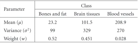
Figure 19 shows a weighted T2 MRI image and its four-modal empirical grey-level distribution approximated with the dominant four-component normal mixture. The four classes represent dark bones and fat, gray matter, white mat-ter, and cerebrospinal fluid (CSF), respectively. The goal is to separate these classes with the minimum classification er-ror. Initial parameters of the dominant mixture are given in Table 7. The Levy distance of 0.11 indicates a large mis-match between the empirical distribution and the dominant

Table6: Final parameter estimates for the dominant Gaussians for

the MRA image inFigure 15a.

Parameter Class

Bones and fat Brain tissues Blood vessels

Mean (µ) 23.2 101.5 208.9

Variance (σ2_{) 99 329 270}

Weight (w) 0.52 0.451 0.028

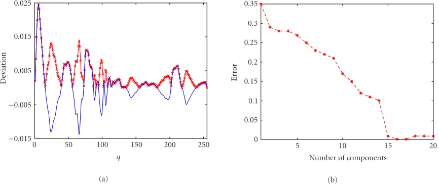
mixture.Figure 20shows the scaled deviations of the dom-inant mixture from the empirical distribution and the changes of the approximation error for the increasing num-ber of components. The minimum error is obtained for the 16 subordinate Gaussians.Figure 21apresents this initial es-timate.

(a)

0 50 100 150 200 250

q 0.004

0.008 0.012 0.016

Densit

y

(b)

Figure19: (a) Typical MRI T2 weighted image and (b) the deviations between the empirical distribution and the dominant mixture.

0 50 100 150 200 250

q

−0.015

−0.005

0.005 0.015 0.025

De

vi

ation

(a)

5 10 15 20

Number of components 0

0.05 0.1 0.15 0.2 0.25 0.3 0.35

Er

ro

r

(b)

Figure20: (a) Estimated subordinate components of the absolute deviation and (b) dynamics of the error as a function of the number of

Gaussians approximating the scaled-up absolute deviation inFigure 20a.

Table7: Initial parameter estimates for the dominant Gaussians for

the MRI image inFigure 19a.

Parameter

Class

Bones and fat

White matter

Gray

matter CSF

Mean (µ) 21.7 82.0 128.6 205.0

Variance (σ2_{) 171.1 192.6 892.7 337.4}

Weight (w) 0.23 0.49 0.19 0.09

distribution and the model decreases to 0.02 from the orig-inal value of 0.11. The minimum classification error of 0.01 on the intersecting distribution tails is obtained for the thresholds t1 = 53, t2 = 110, and t3 = 179 when

the components 1–3, 4–8, 9–12, and 13–16 are assigned to

the first (bones and fat), second (white matter), third (gray matter), and fourth (CSF) classes, respectively. The twenty components of the model are shown in Figure 21c, and the estimated individual models of each class are shown in Figure 21d.

The map refinement process converges after 15 iterations as shown in Figure 22d. The initial and final potentials are shown inTable 8.Table 9shows the final estimated parame-ters for the dominant Gaussians.Figure 22presents the ini-tial and final region maps. The final error is about 3% with respect to the expert’s map inFigure 22c.

4. CONCLUDING REMARKS

0 50 100 150 200 250 q

0 0.005 0.01 0.015 0.02 0.025

Densit

y

(a)

0 50 100 150 200 250

q 0

0.004 0.008 0.012 0.016

Densit

y

(b)

0 50 100 150 200 250

q

−5

0 5 10 15×10

−3

L

C

G

components

(c)

p(q|1) p(q|2)

p(q|3) p(q|4) t1=53

t2=110 t3=179

0 50 100 150 200 250

q 0

0.005 0.01 0.015

Densit

y

(d)

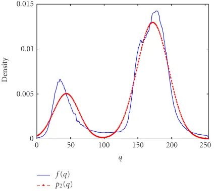
Figure21: (a) Subordinate mixture estimated for the absolute deviation inFigure 20; (b) empirical and estimated densities for the MRI

image inFigure 19a; (c) the model components; and (d) the estimated models of the classes “bones,” “gray matter,” “white matter,” and

“CSF.”

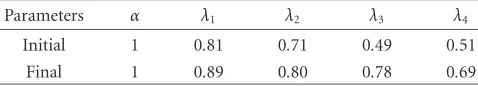
Table8: Initial and final potentials of the map model for the MRI

image inFigure 19a.

Parameters α λ1 λ2 λ3 λ4

Initial 1 0.25 0.15 0.37 0.35

Final 1 0.37 0.29 0.41 0.49

images. The empirical probability distribution of grey lev-els is approximated by a mixture of linear combinations of Gaussians more precisely than by a conventional mixture of Gaussians. This results in a high-quality initial segmentation map that needs only a small refinement by further process-ing based on the joint Gibbs random field model of region

Table9: Final parameter estimates for the dominant Gaussians for

the MRI image inFigure 19a.

Parameter

Class

Bones and fat

White matter

Gray

matter CSF

Mean (µ) 22.9 83.8 125.5 207.0

Variance (σ2_{) 190.1 201.6 780.6 299.4}

Weight (w) 0.22 0.5 0.195 0.085

(a) (b) (c)

2 4 6 8 10 12 14

Iteration

−15

−14.8

−14.6

−14.4

−14.2

−14

Lik

elihood

function

L

(

g,

l

)

(d)

Figure22: (a) Initial and (b) final segmentation by our approach (the final error of 3%); (c) the ground truth by an expert; and (d) the

convergence of the proposed algorithm for the experiment inFigure 19a. The errors are highlighted by the yellow color.

Our experiments confirm that the proposed algorithm segments complex images in some medical applications more precisely than other known techniques. The algorithm is also suitable for approximating different empirical data curves with linear combinations of Gaussians. Future exten-sions will include the like approximation of multivariate den-sities, other Gibbs models for the higher level, and the use of stochastic optimization techniques for estimating the mod-els’ parameters.

REFERENCES

[1] C. A. Glasbey, “An analysis of histogram-based thresholding

algorithms,”CVGIP: Graphical Models and Image Processing,

vol. 55, no. 6, pp. 532–537, 1993.

[2] J. Kittler and J. Illingworth, “Minimum error thresholding,”

Pattern Recognition, vol. 19, no. 1, pp. 41–47, 1986.

[3] N. Otsu, “A threshold selection method from gray level

his-tograms,”IEEE Trans. Syst., Man, Cybern., vol. 9, no. 1, pp. 62–

66, 1979.

[4] N. R. Pal and S. K. Pal, “A review on image segmentation

te-chiniques,”Pattern Recognition, vol. 26, no. 9, pp. 1277–1294,

1993.

[5] O. D. Trier and A. K. Jain, “Goal-directed evaluation of

bina-rization methods,”IEEE Trans. Pattern Anal. Machine Intell.,

vol. 17, no. 12, pp. 1191–1201, 1995.

[6] J. E. Besag, “On the statistical analysis of dirty pictures,”

Jour-nal of the Royal Statistical Society, vol. B48, no. 3, pp. 259–302, 1986.

[7] C. A. Bouman and M. Shapiro, “A multiscale random field

model for Bayesian image segmentation,”IEEE Trans. Image

Processing, vol. 3, no. 2, pp. 162–177, 1994.

[8] R. Chellappa and R. L. Kashyap, “Digital image restoration

using spatial interaction models,”IEEE Trans. Acoust., Speech,

Signal Processing, vol. 30, no. 3, pp. 461–472, 1982.

[9] A. El-Baz and A. A. Farag, “Image segmentation using GMRF

models: parameters estimation and applications,” in Proc.

IEEE International Conference on Image Processing (ICIP ’03), vol. 2, pp. 177–180, Barcelona, Spain, September 2003. [10] A. A. Farag and E. J. Delp, “Image segmentation based on

composite random field models,”Optical Engineering, vol. 31,

no. 12, pp. 2594–2607, 1992.

[11] G. L. Gimel’farb, Image Textures and Gibbs Random Fields,

Kluwer Academic, Dordrecht, the Netherlands, 1999. [12] A. K. Jain, “Advances in mathematical models for image

[13] R. C. Dubes and A. K. Jain, “Random field models in image

analysis,”Journal of Applied Statistics, vol. 16, no. 2, pp. 131–

164, 1989.

[14] A. Goshtasby and W. D. Oneill, “Curve fitting by a sum of

Gaussians,”CVGIP: Graphical Models and Image Processing,

vol. 56, no. 4, pp. 281–288, 1994.

[15] T. Poggio and F. Girosi, “Networks for approximation and

learning,”Proc. IEEE, vol. 78, no. 9, pp. 1481–1497, 1990.

[16] H. W. Sorenson and D. L. Alspach, “Recursive Bayesian

es-timation using Gaussian sums,” Automatica, vol. 7, no. 4,

pp. 465–479, 1971.

[17] A. P. Dempster, N. M. Laird, and D. B. Rubin, “Maximum

likelihood from incomplete data via the EM algorithm,”

Jour-nal of the Royal Statistical Society, vol. 39B, no. 1, pp. 1–38, 1977.

[18] T. K. Moon, “The expectation-maximization algorithm,”

IEEE Signal Processing Mag., vol. 13, no. 6, pp. 47–60, 1996. [19] R. A. Redner and H. F. Walker, “Mixture densities, maximum

likelihood and the EM algorithm (review),”SIAM Review,

vol. 26, no. 2, pp. 195–239, 1984.

[20] M. I. Schlesinger, “Relation between learning and

self-learning in pattern recognition,”Kibernetika, no. 2, pp. 81–88,

1968 (Russian).

[21] M. I. Schlesinger and V. Hlavac,Ten Lectures on Statistical and

Structural Pattern Recognition, Kluwer Academic, Dordrecht, the Netherlands, 2002.

[22] N. E. Day, “Estimating the components of a mixture of

nor-mal distributions,”Biometrika, vol. 56, pp. 463–474, 1969.

[23] D. E. Goldberg,Genetic Algorithms in Search, Optimization

and Machine Learning, Addison-Wesley, Boston, Mass, USA, 1989.

[24] J. W. Lamperti,Probability, John Wiley & Sons, New York, NY,

USA, 1996.

[25] S. Hu, E. A. Hoffman, and J. M. Reinhardt, “Automatic lung

segmentation for accurate quantitation of volumetric X-Ray

CT images,”IEEE Trans. Med. Imag., vol. 20, no. 6, pp. 490–

498, 2001.

[26] C. A. Bouman and B. Liu, “Multiple resolution segmentation

of textured images,”IEEE Trans. Pattern Anal. Machine Intell.,

vol. 13, no. 2, pp. 99–113, 1991.

Ayman El-Bazreceived the B.S. and M.S. degrees in electrical engineering from Man-soura University, Egypt, in 1997 and 2000, respectively. He joined the Computer Vi-sion and Image Processing (CVIP) Lab, the University of Louisville, Kentucky, in May 2001 as a Ph.D. student. During his stay at the University of Louisville, he has been in-volved in the applications of image process-ing and computer vision for medical

age analysis. His current research includes image modeling, im-age segmentation, 2D and 3D registration, visualization, and sur-gical simulation including finite element analysis, where he has au-thored or coauau-thored more than 25 technical articles. Mr. El-Baz is a regular reviewer for a number of technical journals and confer-ences including the IEEE Transactions on Image Processing, and the International Conference on Medical Image Computing and Computer-Assisted Intervention. He was the recipient of the Re-search Louisville Award in 2002 and the Speed School Award for Outstanding Student, Research and Creative Activity in 2003. He is a Member of the IEEE and a Member of Eta Kappa Nu.

Aly A. Farag received his B.S. degree in electrical engineering from Cairo Univer-sity, his M.S. degree in biomedical engi-neering from Ohio State University, Colum-bus, another M.S. degree in bioengineering from the University of Michigan, Ann Ar-bor, and his Ph.D. degree in electrical en-gineering from the Purdue University, In-diana. Dr. Farag joined the University of Louisville, Kentucky, in August 1990, where

he is currently a Professor of electrical and computer engineer-ing. His research interests are concentrated in the fields of com-puter vision and medical imaging. Dr. Farag is the founder and Di-rector of the Computer Vision and Image Processing Laboratory (CVIP Lab), the University of Louisville, which supports a group of more 20 graduate students and postdocs. His contribution has been mainly in the areas of active vision system design, and volume registration, segmentation, and visualization. He has authored or coauthored more than 80 technical articles in leading journals and international meetings in the fields of computer vision and medical imaging. Dr. Farag is an Associate Editor of the IEEE Transactions on Image Processing. He is a regular reviewer for a number of tech-nical journals and to national agencies including the US National Science Foundation and the National Institute of Health. He is a Senior Member of the IEEE and SME, and a Member of Sigma Xi and Phi Kappa Phi.

Georgy Gimel’farb graduated from Kiev Polytechnic Institute, Ukraine, and re-ceived a Ph.D. degree in engineering cy-bernetics from the Institute of Cycy-bernetics, Academy of Sciences of Ukraine, and a D.S. (Eng.) degree in control engineering from the Higher Certifying Commission of the USSR, Moscow, Russia. After working in the Institute of Cybernetics for a long time, Dr. Gimel’farb joined the University of