Shape Changing Transformations: Interactions with Plasticity and Electrochemical Processes

Shape Changing Transformations: Interactions with

Plasticity and Electrochemical Processes

Thesis by

Farshid Roumi

In Partial Fulfillment of the Requirements for the Degree of

Doctor of Philosophy

California Institute of Technology Pasadena, California

2010

c

2010

To my family

Acknowledgments

I never forget anyone who taught me even a word, and my parents were the first to teach me anything, so I should thank them the first. I think at Caltech I have learned how to learn. It was not easy, but it is very rewarding. I feel I can do anything that I want, almost. I, especially, want to thank my advisor Professor Kaushik Bhattacharya, for teaching me some of the most important rules of any profession. I believe he is a professional scientist and I am hoping that I never forget the rules he taught me, especially the one that says: ”Always distinguish between what you are sure is true, with what you expect to be true.” I want to thank Jim Endrizzi and others at International Student Program , especially Jim for answering the complicated questions of an Iranian student. Also I want to thank Natalie Gilmore, and Icy Ma at the Graduate office for being very friendly and helpful. Thanks to Drs. Ken Pickar, Nadia Lapusta and Morteza Gharib for being available when I wanted to ask their opinions. I thank Christine Silva and Cheryl Geer at Thomas building for being very helpful. I also thank my sister Mahshid, and my friends here for helping me have a good social life so I could work better: Branislav Kecman, Shervin Taghavi, Ashley Woodmansee, Luca Giacchino, and many others. I also should not forget Jose, the friendly custodian of Thomas building.

Abstract

Solids undergo phase transformations where the crystal structure changes with temperature, chem-ical potential, stress, applied electric fields, or other external parameters. These occur by either long-range diffusion of atoms (diffusional phase transformation) or by some form of cooperative, ho-mogeneous movement of many atoms that results in changes in crystal structure (displacive phase transformation). In the latter case, these movements are usually less than the interatomic dis-tances, and the atoms maintain their coordination. The most common example of displacive phase transformations is martensitic transformation. The martensitic transformation in steel is econom-ically very important and can result in very different behavior in the product. Other examples of martensitic transformations are shape memory alloys which are lightweight, solid-state alternatives to conventional actuators such as hydraulic, pneumatic, and motor-based systems.

The martensitic transformation usually only depends on temperature and stress and, in contrast to diffusion-based transformations, is not time dependent. In shape memory alloys the transforma-tion is reversible. On the other hand in steel, the martensite formatransforma-tion from austenite by rapidly cooling carbon-steel is not reversible; so steel does not have shape memory properties.

can show different behavior depending on its complex microstructure. Thus understanding the formation mechanisms is crucial for the interpretation and optimization of its properties. As an example, low alloyed steels with transformation induced plasticity (TRIP), metastable austenite steels, are known for strong hardening and excellent elongation and strength. It is suggested that the strain-induced transformation of small amounts of untransformed (retained) austenite into martensite during plastic deformation is a key to this excellent behavior.

Contents

Acknowledgments iv

Abstract vi

Contents viii

List of Figures ix

List of Tables x

1 Introduction 1

2 Martensitic Phase Transformation in the Presence of Plasticity 7

2.1 Introduction. . . 7

2.2 Model . . . 12

2.2.1 Phase-field parameter (order parameter) . . . 13

2.2.1.1 Chemical energy . . . 13

2.2.1.2 Interfacial energy . . . 15

2.2.2 Austenite-martensite phase transformation . . . 15

2.2.2.2 Kinematics compatibility: prediction of A-M and M-M boundaries . 16

2.2.3 Plasticity . . . 18

2.2.3.1 Plastic strain . . . 18

2.2.3.2 Hardening . . . 18

2.2.3.3 Yield criteria . . . 20

2.2.4 Elastic energy. . . 21

2.2.5 Total potential energy . . . 21

2.2.6 Driving forces, equilibrium, and evolution . . . 22

2.2.7 Time-discrete model . . . 23

2.3 Parameters . . . 28

2.3.1 Nucleation barrier . . . 28

2.3.1.1 One- dimension two-well model . . . 28

2.3.1.2 Two-dimension axi-symmetric three-well model. . . 30

2.3.2 Physical range of parameters and scaling . . . 35

2.4 Numerical Exploration . . . 36

2.4.1 Effect of material parameters on the morphology during the quenching process 37 2.4.1.1 Role of transformation barrier . . . 37

2.4.1.2 Role of surface energy . . . 37

2.4.1.3 Role of elastic moduli . . . 39

2.4.1.4 Role of volume change. . . 40

2.4.1.5 Role of plastic deformation . . . 40

2.4.2 Lath microstructure and retained austenite: combined role of volume change

and plasticity . . . 42

2.4.3 Effect of loading on the morphology of the quenched microstructure . . . 43

2.5 Discussions and experimental verifications . . . 43

2.6 References . . . 54

3 Yielding and Overall Plastic Behavior of Orthotropic Polycrystalline Metals 58 3.1 Introduction. . . 58

3.2 Anisotropic plastic behavior of a single crystal. . . 59

3.2.1 Yield criteria . . . 61

3.2.2 Flow rule . . . 63

3.2.3 Hardening . . . 65

3.2.4 Orthotropic behavior: Two slip systems . . . 66

3.2.5 Incremental work function . . . 68

3.3 Overall plastic behavior of a polycrystal . . . 71

3.3.1 Voronoi tessellation . . . 74

3.3.2 Algorithm to estimate overall plastic behavior of a polycrystal . . . 75

3.3.3 Numerical results and discussion . . . 76

3.4 References . . . 78

4 The Role of Size, Geometry, and Mechanical Compatibility in Diffusive Phase Transformations 80 4.1 Introduction. . . 80

4.3 Small and large body limit. . . 88

4.3.1 Small particle limit . . . 89

4.3.2 Large body limit . . . 90

4.4 Thin film limit . . . 96

4.4.1 Transition layers in the thin film limit . . . 102

4.5 Conclusion . . . 105

4.6 References . . . 106

5 General Continuum Mechanics of Elasto-Electro-Chemical Systems with Moving Boundaries 107 5.1 Introduction. . . 107

5.2 Kinematics . . . 108

5.3 Deformable solids with mass transport . . . 109

5.3.1 Conservation of mass. . . 109

5.4 Electrodynamics . . . 111

5.4.1 Space charge density . . . 111

5.4.2 Electric field . . . 113

5.4.3 Discontinuities in the electric field . . . 114

5.5 Rate of dissipation of the system . . . 118

5.6 Elasto-chemical dissipation . . . 119

5.7 Electrical dissipation . . . 121

5.7.1 Rate of change of field energy: step 1 . . . 122

5.7.2 Rate of change of field energy: step 2 . . . 123

5.8 Rate of dissipation: the final expression . . . 127

5.9 Governing equations . . . 130

List of Figures

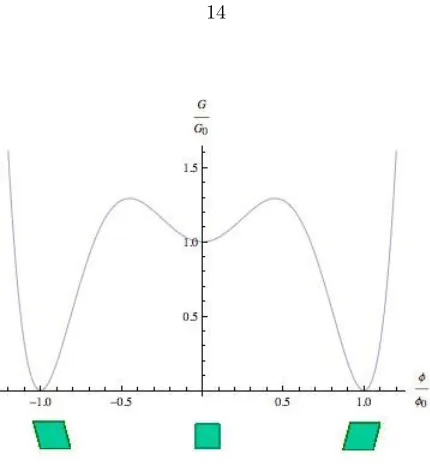
2.1 Chemical energy as a function of the order parameter. φ= 0 means untransformed

austenite,φ=±φ0 indicates the two variants of the transformed martensite. . . 14

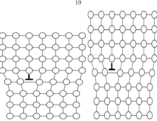
2.2 Phase transformation of a plastic region. Left shows the untransformed austenite.

Right shows the transformed martensite. It is shown that plastic deformation is

in-herited from the old phase on left by the new phase on right. . . 19

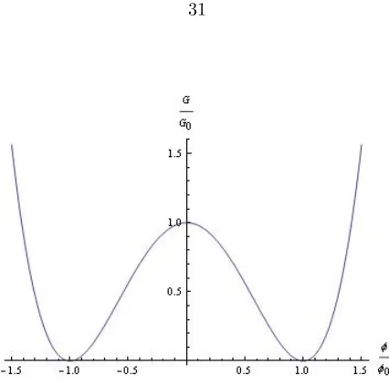
2.3 Simple two-well model. Normalized energy as a function of the normalized order

parameter. . . 31

2.4 Transition zone is defined as the width of the region between φ = 0 and φ = ±φ0.

Transition length depends on the coefficient of the interfacial energy and defined the

physical length scale of the problem. . . 31

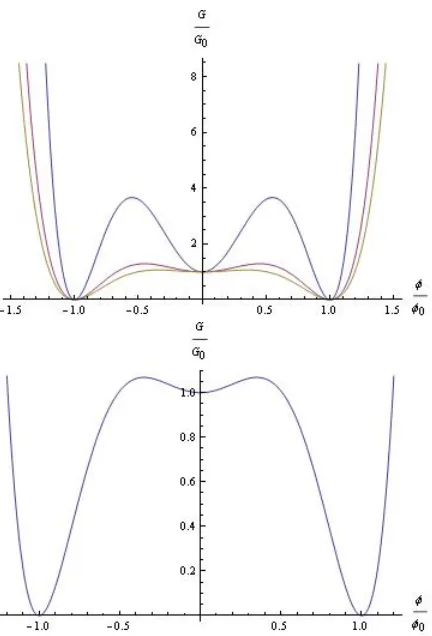
2.5 A three-well model. Left: Normalized energy as a function of the normalized order

parameter for different values of α = 0.55,0.45,0.35. Right: A closer look at the

2.6 Martensitic transformation upon quenching. Volume change=0, average strain=0.

Here we show some middle time steps,t= 0,16,20,30 and not the final morphology.

The color bar shows the order parameter. We observe that the stress field due to the

neighboring nuclei plays a key role on how a nucleus grows into a plate of a specific

thickness dictated by minimizing the sum of the elastic energy and surface energy. . . 38

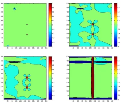
2.7 Martensitic transformation upon quenching. Volume change=0.08, average strain=0.

When the transformation barrier or the coefficients of surface energy or elastic energy

are very high (right figure) the energy barrier can get too high and the material

would prefer to stay at the metastable austenite phase (green) instead of the twined

martensite structure (red and blue). . . 39

2.8 Martensitic transformation upon quenching. Volume change=0.08, average strain=0.

Here we show some middle time steps,t= 0,16,20,30 and not the final morphology.

The color bar shows the order parameter. Here we observe that the stress field due

to one nucleus results in the nucleation of the other variant. We further observe the

twined plates which grow together and nucleate more plates. . . 41

2.9 Effect of plasticity: Observed twinning and retained austenite in the final morphology,

a simple cartoon . . . 42

2.10 Martensitic transformation with no volume change, average strain=0, no plasticity,

average surface energy. In the absence of volume change and plasticity, the material

makes long twined plates of martensite to minimize the total elastic energy. The

2.11 Martensitic transformation with no volume change, average strain=0,σy= 200 MPa,

average surface energy. In the absence of volume change, the plasticity reduces the

deviatoric and total stresses and thus reduces the elastic energy barrier to

transforma-tion, and thus makes the transformation easier. The material still makes long twined

plates of martensite to minimize the total elastic energy. The surface energy forces

the morphology to be a coarse one.. . . 45

2.12 Martensitic transformation with volume change=0.08, average strain=0, no plasticity,

average surface energy. Volume change causes higher stresses and thus higher elastic

energy barrier in the material, and thus makes the phase transformation slower. The

boundary conditions, average strain=0, results in higher stresses in general, and thus

the phase transformation stops as the driving force from the chemical energy difference

between the austenite and martensite is not enough to overcome the elastic energy

barrier. . . 46

2.13 Martensitic transformation with volume change=0.08, average strain=0, σy= 200

MPa, average surface energy. Volume change causes higher stresses and thus higher

elastic energy barrier in the material, and thus makes the phase transformation slower.

On the other hand plastic deformation reduces the deviatoric stresses and thus makes

the transformation easier. The boundary conditions, average strain=0, results in

higher stresses in general. In this case the competition between lower deviatoric stress

due to plastic deformation and higher volumetric stresses due to volume change results

2.14 Martensitic transformation with volume change=0.08, average stress=0, no plasticity,

average surface energy. Volume change causes higher stresses and thus higher elastic

energy barrier in the material, and thus makes the phase transformation slower. . . . 48

2.15 Martensitic transformation with volume change=0.08, average stress=0, σy= 200

MPa, average surface energy. Volume change causes higher stresses and thus higher

elastic energy barrier in the material, and thus makes the phase transformation slower.

On the other hand plastic deformation reduces the deviatoric stresses and thus makes

the transformation easier. The boundary conditions, average stress=0, results in lower

stresses in general. The phase transformation completes. . . 49

2.16 Martensitic transformation with volume change=0.08, average strain=0, σy= 200

MPa, average surface energy. It is observed that the combination of the volume

change at plastic deformation results in a complex morphology including regions of

twining and retained austenite). Due to plastic deformation the preferred angle

be-tween austenite and martensite differs from that of the no plastic case∼6◦. . . 50

2.17 Martensitic transformation with volume change=0.08, average stress=0, σy= 200

MPa, low surface energy. It is observed that the combination of the volume change at

plastic deformation results in the presence of some untransformed regions of austenite

(retained austenite). Due to plastic deformation the preferred angle between austenite

2.18 Martensitic transformation with volume change=0.08, average strain=0, σy= 200

MPa, low surface energy. With applied 0

12 = 0.1. It’s observed that upon

apply-ing far-field strain, the material tries to accommodate it by increasapply-ing the volume

fraction of the preferred martensite variant at the expense of reduction of the other

variant. We also see that some of the retained austenite transforms to the preferred

martensite variant. . . 52

3.1 Stress-strain curve for different steels compared to aluminum according to United

States Steel Corporation . . . 60

3.2 Stress-strain curve for martensite, TRIP steel, and austenite . . . 61

3.3 A schematic figure showing lath microstructure: martensitic layers (blue), with

re-tained austenite (white) between them. . . 68

3.4 Optical micrographs of lath martensite in (a) Fe-0.0026C, (b) Fe-0.18C, (c) Fe-0.38C

and (d) Fe-0.61C alloys. Etching solution: 3% nital. Morito et al. (2005) . . . 72

3.5 Voronoi tessellation . . . 75

3.6 Estimated mechanical behavior of the polycrystal for different values of domain sizes,

n×n, and number of grainsnG. n= 200 for seriesAandB,n= 400 for series C and D.nG= 1 for series A,nG= 10 for seriesB andC. nG= 20 for series D. SeriesA

shows the orthotropic behavior of a single grain. . . 77

5.1 A discontinuity separating two regions. Each region can have different elastic or

List of Tables

3.1 Yield strength, ultimate strength and total elongation of mild steel, TRIP steels, and

Chapter 1

Introduction

Solids undergo phase transformations where the crystal structure changes with temperature, chem-ical potential, stress, applied electric fields, or other external parameters. These occur by either long-range diffusion of atoms (diffusional phase transformation) or by some form of cooperative, ho-mogeneous movement of many atoms that results in changes in crystal structure (displacive phase transformation). In the latter case, these movements are usually less than the interatomic dis-tances, and the atoms maintain their coordination. The most common example of displacive phase transformations is martensitic transformation. The martensitic transformation in steel is econom-ically very important and can result in very different behavior in the product. Other examples of martensitic transformations are shape memory alloys which are lightweight, solid-state alternatives to conventional actuators such as hydraulic, pneumatic, and motor-based systems.

The martensitic transformation usually only depends on temperature and stress and, in contrast to diffusion-based transformations, is not time dependent. In shape memory alloys the transforma-tion is reversible. On the other hand in steel, the martensite formatransforma-tion from austenite by rapidly cooling carbon-steel is not reversible; so steel does not have shape memory properties.

transformation interactions with plastic deformations. A good example here is steel, which has been known for thousands of years but still is believed to be a very complicated material. Steel can show different behavior depending on its complex microstructure. Thus understanding the forma-tion mechanisms is crucial for the interpretaforma-tion and optimizaforma-tion of its properties. As an example, low alloyed steels with transformation induced plasticity (TRIP), metastable austenite steels, are known for strong hardening and excellent elongation and strength. It is suggested that the strain-induced transformation of small amounts of untransformed (retained) austenite into martensite during plastic deformation is a key to this excellent behavior.

In the second chapter, we investigate the morphology of martensitic phase transformation in the presence of plasticity. Using a phase field model, we introduce the total energy of the system as a function of an order parameter which is correlated with the transformation strain, and address the effect of elasticity, volume change, nucleation barrier, and plastic deformations on the morphology of the transformation.

Our numerical simulations suggest that the volume change of the transformation is responsi-ble for the observed fine microstructure of martensite which has been observed in lath steel. It also suggests that the interactions between plasticity and phase transformation result in pinning of the martensitic transformation and presence of untransformed regions of retained austenite. As a conclusion, in agreement with experimental observations in steel, our simulations suggest that the interactions between plasticity and the volume change are responsible for the observed fine martensite microstructure with retained austenite known as lath microstructure.

polycrys-talline metals. There is always a tradeoff between hardness and toughness in materials. Here we show that small fractions of soft yet tough layers between hard but brittle layers can result in a hard and tough overall behavior even in the polycrystal. One example is layers of austenite between martensite layers in lath microstructure which is observed in steel. Based on Hill’s anisotropic plas-ticity model, we use a rate-independent, strain hardening orthotropic, associate plasplas-ticity model for each single crystal and estimate the overall plastic behavior of a polycrystal. As the conclusion to the first part of this work, we identify the low-yield strength austenite and high volume changes of transformation as the underlying microstructure resulting in the hard and tough behavior of the polycrystalline observed in experiments.

In the fourth chapter, using asymptotic limit analysis, we study the effects of geometry and size of electrodes on elastic energy and concentration profile. We consider the state of lowest free energy of the system; although in practice, due to kinetics, defects, etc., the material may be at a metastable state of energy and may not reach its lowest free energy. Here, we use a phase-field model to estimate the behavior of the elasto-electro-chemical system. The surface energy is modeled as a function of the space gradients of the li-ion concentration, which plays an important rule in describing the concentration profile for different sizes and geometries. The electrochemical energy is modeled as a double-well function with minima near fully lithiated and delithiated states. The elastic energy, assuming coherent interfaces, is a function of the phase transformation between lithi-ated and delithilithi-ated phases, e.g., orthorhombic to orthorhombic phase transformation inLiF eP O4.

It can also be a function of the applied displacement and traction boundary conditions from the charge collector and electrolyte. It is expected that the elastic energy can play an important role by making the transformation barrier higher and thus limiting the rate. It can also be a major player in the life cycle of the system. This means that one should make the crystallographic changes in electrodes as compatible as possible in order to have higher rates and more cycles. One other import issue is that, when the gradient energy term is large compared to the electrochemical en-ergy, the system does not obey Fick’s law. This could occur, for example, across an interface in inhomogeneous systems in which the concentration profile is characterized by a strongly varying curvature. In this case, one has to do a more general study to understand the system and predict its behavior.

a) Small body limit: in this limit, we prove that in very small particle limit the concentration profile should be of a single domain in each particle. This results in the elimination of the elastic energy for very small particles. The reduced energy barrier suggests higher rates as suggested by recent experiments and also possibly longer life of the battery. Our results show that for very small particles we should have only either fully lithiated or fully delithiated particles, as reported by experiments of Delmas and some other groups, thus the overall behavior of the concentration, as an averaging scheme, can show reduced miscibility gap.

b) Large body limit: in this limit we prove that we should see multiple layers of lithiated and delithiated phases adjacent to each other in a preferred direction in order to minimize the elastic energy. This is again in accordance with several experiments on large domains.

c) Thin film limit: In this limit we show that the concentration profile should be uniform in the thickness, though depending on the other dimensions of the film it can show periodic layers of lithi-ated and delithilithi-ated phases with a preferred normal direction. This is also consisted with recent experiments of thin films ofLiF eP O4.

Chapter 2

Martensitic Phase Transformation

in the Presence of Plasticity

2.1

Introduction

Martensitic phase transformation is a diffusionless, solid-to-solid, structural phase transformation from a high-temperature phase, austenite, to a low-temperature phase, martensite. The resultant martensite structure shows itself as multiple symmetry-related variants of martensite which are oriented differently with respect to the austenite lattice but have identical crystal structure. This is because the high-temperature austenite phase often has greater symmetry than the low-temperature martensite phase (Bhattacharya 2003).

orientation due to fewer crystallographic symmetries after transformation. This transformation, initiated by sudden cooling (quenching), results in enormous shear strains and the product usually avoid these intolerable strains by either slipping (plastic deformation) or twinning. The combina-tion of transformacombina-tion and plasticity leads to complex microstructures. Specifically, it has been proposed that plastic accommodation causes the technologically important plate-lath morpholog-ical transition in steels (Olson and Cohen 1986). This transformation plays a critmorpholog-ical role in the resulting hardness of steel. This is the motivation for our model.

The competition of plasticity and the phase transformation results in different types of marten-site in steel. Austenite yield strength is about 2–3 times less than martenmarten-site. If plasticity can happen before the phase transformation, then we see lath martensite, which is the combination of plastic strains and transformation strains. If the yield strength of martensite is so high that plas-ticity doesn’t happen, we see plate martensite. Yield strength depends on the carbon content, the higher the carbon content, the higher the yield strength, and so we expect to see plate martensite with very sharp and straight interface, as elasticity is scale-less; however, when there is plastic-ity involved, we see a very complicated interface (surprisingly enough in this case the higher the carbon the more complicated the boundary) which may be due to another mechanism of carbon atom movements. Adding more carbon not only gives more resistance to yielding, but by also strengthening austenite, it makes the transformation harder, and so we need more energy in this case, resulting in lowerMs. This might be due to the fact that more carbon results in biggerc/a,

where (a, a, c) are the dimensions of the martensite unit cell, c > a, noting that carbon offset in theb.c.t.is the cause of lengthening in one direction. It seems that growth of martensite embryos happens first by elongation until stopped by an obstacle, and then by thickening of martensite.

martensites in steels. That group found that twin-related martensite variants do not favor the retention of austenite. They observed that inter-martensite austenite films were most likely seen when the adjacent martensite variants were in the same crystallographic orientation. They also suggested there would be less retained austenite between twin related variants of martensite. In

F e−4N i−0.4C, the observed retained austenite films were about 1% and rather discontinuous. InF e−3.9M o−0.18Cinter-martensite retained austenite films were very fine, but their quantity was considerable. InF e−0.08C−1.1M n−0.2Si−5.5N i−14.5Cr−2.1M o−0.7N b−1.9Cu, they observed large quantities of heavily faulted austenite. In F e−0.31C−2.0Si the alternate martensite laths were twin related, and they didn’t find any retained austenite.

Wayman and co-workers (1976, 1992) studied the crystallography and morphology of ferrous martensite. For plate substructure, they observed that the parallel sided plates are characterized by an internal structure consisting of a single set of twins that sometimes extends completely across the plate to the interfaces. Stronger austenite results in finer martensite twins. ForF e−N ialloys, they reported segmented and irregular plates, a central region of twins, and arrays of skew dislocations in the peripheral regions (for example inF e−29N ithey reported no twins, however they saw fully twinedF e−34N ialloys). Constancy of the shape change across the plate width implies that the lattice invariant strain is constant and changes from slip to twinning. They suggested the change to be due to a local temperature rise at the interface during growth.

Growth of individual sub-plates and macroscopic plates is accompanied by intense accommodation slip in the austenite on the particular (111)F plane that is nearly parallel to the habit plane.

The experimental observations suggest that at first the inclusion grows longitudinally, and then after reaching the borders of the austenite grain or any other constraint, say the borders of other inclusions, it thickens.

Maki and co-workers (2005) studied F e−N i alloys and concluded that martensite inherits plasticity from austenite. They also observed that there is no plasticity in the mid-rib, twined plate, but the area around the lath is highly plastic, and suggested that plasticity begins after the formation of the mid-rib. They (2006) also studied F e−N i−Co alloys and observed that for smaller volume changes, there is less dislocation density, and the M/A interface is smoother. They observed that in non-ferrous alloys, if volume change is about zero, we only have plate martensite; but in ferrous alloys, we might see lenticular too. They suggested that smaller volume change and lowerMsresult in more lenticular, while more volume change and moreMs gives more lath. They

measured the dislocation density in the order of 1015_m−2 _{for lath martensite.}

the phase field method to coherent transformations in solids by considering transformation-induced coherency strain. Wang and Khachaturyan (2006) extended the early phase field model of Cahn to arbitrary microstructures with arbitrary transformation strains using the microelasticity theory of Khachaturyan and Shatalov (1967, 1969, 1983).

When the conditions for thermo-elastic growth are not met, plastic accommodation of the trans-formation shape strain may be substantial. In this case the interaction between a growing martensite plate and its plastic zone becomes important, determining the growth path of a martensite inclusion. Despite of the approximate treatment of the stress-strain fields, the first model of martensitic plate growth in the plastic regime (Olson and Cohen 1985, Haezebrouck 1987) studied the longitudinal growth arrest due to plastic accommodation. Marketz and Fischer (1994) did a finite-element sim-ulation of nucleation and growth of a martensitic plate. Wen et al. (1999) obtained a finite-element solution for modeling the growth by discrete martensitic layers. They modeled the transformation in each layer by homogeneous growth of the transformation strain from zero to its final value, and proposed a PT criterion and an extremum principle to choose the next transforming layer. However, kinetic equations were not implemented in these works. Levitas and co-workers (1999, 2002) developed a mesoscopic continuum thermo-mechanical theory of martensitic phase transi-tion in inelastic materials and studied the problem of the appearance of a martensitic plate in an elastoplastic austenitic matrix at finite strains. However they were restricted to fixed aspect ratios and neglected the inter-inclusion interactions. As many other works, they have used some empirical relations based on best fit with a reference experiment, and therefore their works are only applicable to some specific material-environment conditions.

plate martensite. When lath martensite is formed inF e−29wt%N iat 266− −133K, the evolved heat corresponds to an enthalpy of transformation∼1600J/mole independent of transformation temperature and volume fraction (Tamura and Wayman 1992). This is similar to enthalpy change forF e−30.3wt%N itransformed at 243−−198K. But at lower temperatures where plate martensite is formed, it is more than 2600J/mole. Noting that the stored energy due to the dislocations is very low, Christian (1979) suggested that the difference is due the better elastic accommodation of the plates. For anF e−13.7%N i−0.86%Csteel transformed at 297−188K, as the volume fraction changes from 7 to 59%, the measured enthalpy change at 507Kdecreases from 4650 to 1600J/mole. Christian suggested that the increase in the stored energy is due to high work-hardening and high dislocation densities in the regions of deformed austenite which have subsequently to be transformed to martensite.

Despite the detailed experimental observations, idealized theoretical models, and empirical rules in the literature, there is a lack of a complete microstructure study. There are discrepancies with different models, and the role of plasticity is not understood throughly. We seek to develop a model that describes microstructure development during quenching and to determine the criteria for the resulted microstructure change from plate to lath with retained austenite. We then study the effect of loading on the quenched system to understand the mechanism of concurrent toughening and hardening observed in some materials, such as steel. We limit ourselves to two-dimension, small strains, 2 variants of martensite.

2.2

Model

strains and plastic strains. We assume that there are three major contributions to the free energy. The first is the interfacial energy on interfaces separating different phases. Second is the chemical energy which prefers the martensite state to the austenite state at the temperature of interest. Finally, the third is the elastic energy. Plastic strain is governed by a Mises yield criteria and Ramberg-Osgood isotropic hardening.

2.2.1

Phase-field parameter (order parameter)

We study the austenite-martensite phase transition in the presence of plasticity by introducing a phase field model. A key model in the phase field model of our problem is to formulate the total free energy of the system as a function of the order parameter,φ, such that φ =±φ0 stands for

different martensite variants (twins), andφ= 0 stands for austenite.

2.2.1.1 Chemical energy

G(φ), the chemical free energy of a homogeneous system is usually approximated by a Landau polynomial expansion with respect to the order parameter. We model it by a three-well function with minima at austenite, and 2 martensite variants. In our model austenite is assumed to be less stable than martensite due to undercooling caused by quenching.

G(φ) =G(0) 3α

2_−β2_−2φ2

β2_−φ22

3α2_β4_−β6 , (2.1)

differentiating with respect to the order parameter gives

∂G(φ)

∂φ =G(0)

−12φ(φ2−α2)(φ2−β2)

Figure 2.1: Chemical energy as a function of the order parameter. φ = 0 means untransformed austenite,φ=±φ0 indicates the two variants of the transformed martensite.

αand β are the local maximizer and minimizer of G(φ). G(φ= 0) is the undercooling, chemical driving force. The activation energy (barrier energy),A, is then

A=G(0)

_(α2_−β2₎3

b4_(3α2_−β2₎−1

. (2.3)

As we have assumed the wells to be atφ= 0,±φ0, and austenite to be less stable than martensite,

we haveβ =φ0 and 0<a˜=a/φ0<0.577 and

A=G(0)

(˜a2−1)3 3˜a2₋₁ −1

. (2.4)

2.2.1.2 Interfacial energy

The gradient term, λ₂2|∇φ|2_{accounts for rapid changes ofφor the interface between different phases.}

Its role is to suppress any oscillation that would occur when solving for the other two terms and thus may be regarded as interface energy. This interfacial energy penalizes abrupt changes in the system by making a transition zone, however this transition zone may not be significant in reality, and we may see a sharp interface between austenite and martensite states, as in plate martensite. In this case, the introduced interfacial energy is a mathematical term to correctly connect the energies in micro scale to thecontinuum scale, while it does not change the overall pattern or affect the overall behavior if the computational domain is large enough. Here, the parameterλ2describes the length scale of the numerical simulations and is usually determined by either fitting of interfacial energies to experimental results or by using first principles.

2.2.2

Austenite-martensite phase transformation

2.2.2.1 Transformation strain

We assume the transformation strain, a function of order parameterφ, as:

T =

   

γφ2 _ηφ

ηφ γφ2

   

. (2.5)

Typical values for transformation strain of steel, are 0.02− −0.05 volumetric transformation strain and 0.20 transformation shear. Assuming the order parameter φ= ±0.2 for martensite variants, we haveγ andη of ordero(1).

2.2.2.2 Kinematics compatibility: prediction of A-M and M-M boundaries

Continuity of the displacement at the boundary of two different phases requires the difference in their derivatives to be of rank one. Mathematically it means that ifFandGare the deformation gradients in two adjacent regions, there should exist vectorsaand ˆnsuch that (Bhattacharya 2003),

Fij−Gij = 2ainj. (2.6)

This requires the difference in the symmetric part of the derivatives, strain tensors, to satisfy the following equation:

In the case of infinitesimal strains, definingλi, and ei as the eigenvalues and eigenvectors of ∆,

the interface will be possible ifλ1> λ2= 0> λ3. In this case we can find the vector ˆnfrom

ˆ

n=±√λ1e1+ √

λ2e2. (2.8)

Consider the two dimension case of our problem. We only consider the transformation strain, as it is the major component of the strain, compared to elastic strains. For the boundary between two adjacent martensite regions we have

tr₁ =

   

φ2 ηφ

ηφ φ2

    (2.9) and

tr₂ =

   

φ2 −ηφ

−ηφ φ2

   

(2.10)

so we will get

∆=

   

0 2ηφ

2ηφ 0

   

. (2.11)

The eigenvalues and eigenvectors of this matrix areλ= 2φ,−2φande= (1/p(2),±1/p(2)), so we will haven=±(1/p(2),−1/p(2)) + (1/p(2),1/p(2)) son= (0,1) or (1,0). So in 2D, martensite variants form right angles with each other.

will have

∆=

   

φ2 ηφ

ηφ φ2

   

(2.12)

which has λ = φ2±φ, and e = (1,±1). If we substitute φ = .2, the the austenite/martensite interface will be about ±6 or 84◦. We saw that in two dimensions A/M interface is possible. However making an austenite/martensite interface is not possible in a three dimension case. This is the reason for laboratory-observed microstructure in steels. In this case the interface will be between austenite and twinned martensite.

2.2.3

Plasticity

It is believed that plasticity plays an important role in the irreversibility of the phase transformation and also the observed hard and tough behavior of some steels. Here, we define a rate-independent isotropic hardeningJ2 plasticity model.

2.2.3.1 Plastic strain

Our main assumption is that martensite is much harder than austenite, so we assume linear elastic behavior for martensite variants, and strain hardening,J2plasticity model for austenite. We further

note that plasticity,p_{, is transferred from austenite to martensite, so the total inelastic strain at}

each point istr₊p_{, as shown in Figure 2.2.}

2.2.3.2 Hardening

The stored cold work energy,Wp₍nl_{, q), is the non-elastic part of the free energy which depends}

Figure 2.2: Phase transformation of a plastic region. Left shows the untransformed austenite. Right shows the transformed martensite. It is shown that plastic deformation is inherited from the old phase on left by the new phase on right.

Here we assumeq=p_M is the Mises strain. We assume a power-law form for the stored mechanical energy as follows, assuming only isotropic hardening

Wp p_ij, p_M

= n

p 0

n+ 1σ0

1 +

p M

p₀

n+1n

(2.13)

from which the yield stress is

σy=

∂Wp(p, p_M)

∂p_M =σ0

1 +

p M

p₀

1n

(2.14)

the back stress of kinematic hardening vanishes:

σ∗= ∂W

p₍p_, p M)

In the limit whenn−→ ∞, we have perfect elastic-plastic behavior

σy −→σ0

1 +

p M

p₀

0

=σ0. (2.16)

2.2.3.3 Yield criteria

The Mises yield criterion suggests that the yielding of materials begins when the second deviatoric stress invariantJ2 reaches a critical value. This implies that the yield condition is independent of

hydrostatic stresses.

f(J2) =

p

J2−k= 0, (2.17)

wherekis the yield stress of the material in pure shear.

Applying a uniaxial stress, it is seen that, at the onset of yielding, the magnitude of the shear yield stress in pure shear,k, is√3 times lower than the tensile yield stress in the case of uniaxial tension,σy. Thus, we have

k=√σy

3. (2.18)

The Mises yield criterion can be expressed as:

f(J2) =

p

3J2−σy= 0. (2.19)

SubstitutingJ2as a function of the stress tensor components

(σ11−σ22)2+ (σ22−σ33)2+ (σ33−σ11)2+ 6(σ232 +σ 2 31+σ

2 12) = 6k

2_{= 2σ}2

which defines the yield surface as a circular cylinder whose intersection with the deviatoric plane, is a circle with radius√2k, or p2/3σy.

We assume plane stress in our model so we have σ33=σ31=σ32= 0.

2.2.4

Elastic energy

We assume infinitesimal elastic deformations and identical isotropic behavior by all phases; so we can write the elastic energy density as

W1 , pl, pt(φ)= 1 2 −

pt₋pl

:C: −pt−pl. (2.21)

2.2.5

Total potential energy

Putting the aforementioned energy terms together, we postulate the energy functional density as the sum of the four terms in the following form:

U =λ

2

2 | ∇φ|

2_{+G(φ) +}1

2 −

pt₋pl

:C: −pt−pl+Wp(pl, plM), (2.22)

from which the total energy of the system is

E=

Z

Ω

2.2.6

Driving forces, equilibrium, and evolution

Here we assume that the material is always at the state of stress equilibrium, so minimizing the Lagrangian of the total free energy with respect to the strains gives

∇. _C: (−pt−pl)

= 0. (2.24)

The driving force for the phase transformation, order parameter, is assumed to be the change of the total free energy with respect to the order parameter

dφ=−

∂E

∂φ. (2.25)

The spatial evolution of φ, which completely defines the microstructural evolution during phase transformation is obtained by assuming a linear dependence of the rate of deformation on the driving force

˙

φ=−∂E

∂φ. (2.26)

Equations in this format are widely used to study various problems of microstructure evolution. We get the following evolution equation:

˙

φ=λ2∆φ−G0(φ) + −pt−pl

:_C: ∂

pt

∂φ −

∂Wp

Similarly we have

dpl=−

∂E

∂pl, (2.28)

so we have

dpl ij

=_C: −pt−pl

ij−

∂Wp

∂p_ij =σ

dev

ij −σ∗ij, (2.29)

where in the second equation, we have made the assumption of no volume change due to plasticity in metals, and defined the deviatoric part of the stress tensor asσdev

ij . σ∗ is the back stress. Here

for simplicity we neglect kinematic hardening, soσ∗=0.

2.2.7

Time-discrete model

To study the above model numerically, we introduce a time discretization and seek an implicit formulation, (Stainier and Ortiz 1999). To this end, we introduce the incremental work function to be:

Fn

n+1, pln+1, φn+1

=

Z

Ω

fndΩ, (2.30)

where

fn=Un+1

n+1, pln+1, φn+1

−Un n, pln, φn+ ∆t ψ∗

pl_n+1−pl n

∆t ,

φn+1−φn

∆t

!

, (2.31)

whereψ∗ is the dual kinetic potential.

plastic and internal variable dissipation:

ψ∗

pl n+1−pln

∆t ,

φn+1−φn

∆t

!

=ψ∗p

pl n+1−pln

∆t

!

+ψ∗φ

_φ

n+1−φn

∆t

. (2.32)

Given n, pln, φn, we minimize Fn with respect to n+1, pln+1, φn+1. Minimization with respect to

n+1 gives the mentioned equilibrium equation (2.24).

Minimization ofFn with respect to the plastic strain at each state gives:

δpl n+1

Fn = 0. (2.33)

This can be written as

∂Un+1

∂pl_n+1 + ∆t ∂ψ∗

∂pl_n+1 =−(Y

p₎ n+1+

∂ψ∗p

∂˙pl_n+1

pl_n+1−(pln

∆t

!

= 0. (2.34)

In the above formula, the driving force with respect to the plastic strain is defined as:

Yp=−∂U

∂pl =C −

pt_(φ)−pl

−∂W p

∂pl =σ−σ

∗_{, (2.35)}

and

∂ψ∗

∂˙ =σ−σ

∗_{, (2.36)}

where

σ∗=∂W

p _, pl

Finally, minimization with respect to the order parameterφgives:

δφn+1Fn = 0, (2.38)

or equivalently

∂Un+1

∂φn+1

+ ∆t ∂ψ ∗

∂φn+1

=− yφ

n+1+

∂ψ∗φ

∂φ˙n+1

_φ

n+1−φn

∆t

= 0, (2.39)

where driving force for the order parameterφis defined by:

yφ=−∂U

∂φ =−

∂W1 _, pl_{, φ}

∂φn+1

+4φn+1−

∂Gc(φn+1)

∂φn+1

. (2.40)

This can be further simplified as

yφ= −∂W

1 _, pl_, pt_(φ)

∂pt_(φ) n+1

∂pt_(φ n+1)

∂φn+1

+4φn+1−

∂G(φn+1)

∂φn+1

(2.41)

=σn+1

∂pt_(φ n+1)

∂φn+1

+4φn+1−

∂G(φn+1)

∂φn+1

.

Now, assume there exists a kinetic potentialψφ_{, such that we can write its dual potential as:}

ψ∗φφ˙=1 2 ˙

φ2. (2.42)

Differentiating with respect to the rate of change of the order parameter gives

∂ψ∗φ

∂φ˙n+1

_φ

n+1−φn

∆t

=φn+1−φn

which shows that the suggested dual potential satisfies the assumed material kinetics rule

φn+1−φn

δt =σ

∂(tr_(φ)) n+1

∂φn+1

+4φ−∂Gc(φn+1)

∂φn+1

(2.44)

which is the implicit form.

Note that the dual potentials are derived from applying the backward-Euler algorithm to the following kinetic relations:

p_n+1−p n

∆t =

∂ψp

∂Yp (Y p₎

n+1

(2.45)

and

φn+1−φn

∆t =

∂ψφ ∂yφ

yφ_n+1. (2.46)

Now, considering the dual kinetic potential of the plastic dissipation, we have

σ−σ∗= ∂ψ ∗p _˙pl

∂˙pl . (2.47)

Define an effective (Mises) plastic strain as

p_M =

r

2 3

p ij

p

ij 3−dimension,

p

M =

q

It can be shown that a rate dependent plastic dual potential can be written as

ψ∗p ˙pl

=       

∞, ˙p_M <0

g∗ ˙pl

, ˙p_M ≥0

, (2.49)

where g∗ is a function of the plasticity invariants (J1 ˙pl

, J2 ˙pl

, J3 ˙pl

). Now, if we assume that we are interested inJ2 plasticity this simplifies as

g∗ ˙pl

=g∗ J2 ˙pl. (2.50)

Let’s assume a power-law rate dependent plasticity model

g∗ ˙pl

= km˙

p 0

m+ 1σy

_˙p

M

˙

p₀

mm+1

. (2.51)

Then, for ˙p_M >0 we will get

σ−σ∗= ∂g ∗p_{( ˙}p₎

∂˙p =kσy

_˙p M ˙ p₀ m1 (2.52)

which is equivalent to

˙

p_M = ˙pl₀

_σ−σ∗

kσy

m

. (2.53)

Finally we assume the stored energy of the cold work

where the dependence ofWp _onpl

ij gives the kinematic hardening, and its dependence on q gives

the isotropic hardening behavior in whichqis an internal variable. A suitable choice for qcan be

q=

Z

˙

p_Mdt or q=p_M. (2.55)

So, we have shown that the proposed variational form satisfies all kinetics rules. In the numerical experiment section we use the incremental formulation described here with the energies and plas-ticity models described earlier. We further use a rate-independent plastic dissipation model. We use the values defined in the following section.

2.3

Parameters

2.3.1

Nucleation barrier

To understand the effect of nucleation barrier and deciding on the range of it in our model (Figures

2.3and 2.5) , we do a simple one-dimension model, and then extend the results to two dimensions.

2.3.1.1 One- dimension two-well model

We seek to understand the interfacial energy and interfacial width. For simplicity assume we work in one- dimension and neglect elastic energy comparing to the other terms. We idealize and assume to have

G(ϕ) =κ 4 ϕ

2_−ϕ2 0

2

= κ 4ϕ

4 0 ϕ˜

2₋₁2

where ˜ϕ=ϕ/ϕ0. Adding the gradient term,

f =λ

2

2 ϕ

2

,x+G(ϕ) =

λ2 2 ϕ 2 ,x+ κ 4 ϕ

2_−ϕ2 0

2

=ϕ2₀λ

2

2 ϕ˜

2 ,x+

κ

4ϕ

4 0 ϕ˜

2₋₁2

(2.57)

we get

˙

ϕ=λ2ϕ,xx−κϕ φ2−ϕ20

or ϕ0ϕ˙˜=ϕ20λ 2_ϕ˜

,xx−ϕ30κϕ˜ ϕ˜ 2

−1

. (2.58)

The stationary solution of this ODE is obtained by setting ˙ϕ= 0. Assume the solution to be of the form

ϕ=a tanh(x

x0

). (2.59)

So

ϕ,xx=−2a

sinh(_xx

0)

x2₀cosh3₍x x0)

, (2.60)

or

−2aλ2 sinh(

x x0)

x2 0cosh3(

x x0)

−kasinh(

x x0)

cosh(_xx

0)

(a2sinh

2₍x x0)

cosh2₍x x0)

−ϕ2₀) = 0, (2.61)

and

−2λ2

x2 0

−k

a2sinh2(x

x0

)−ϕ2₀cosh2(x

x0

)

Usingcosh2_x−sinh2_{x= 1 we get}

a=ϕ0 and

2λ2 x2

0

=kϕ2₀→x0=

1

ϕ0

r

2α2

k , (2.63)

and

ϕ=ϕ0 tanh

 

ϕ0x

q

2λ2

κ



. (2.64)

The energy is

E0=

Z ∞

∞

f(ϕ(x))dx=ϕ2₀2

3

s

2λ2

κϕ0

2λ2+κϕ2₀. (2.65)

This energy is associated with an interface of the approximate width of

L'4ϕ0

r

2λ2

κ . (2.66)

2.3.1.2 Two-dimension axi-symmetric three-well model

The required energy for the growth of a nuclei of radius ris the surface energy minus the change in the chemical potential:

Figure 2.3: Simple two-well model. Normalized energy as a function of the normalized order parameter

Figure 2.4: Transition zone is defined as the width of the region between φ = 0 and φ = ±φ0.

whereγis the surface energy. To find the critical value ofr

dE

dr =γ−r

∗_{G(0) = 0 =⇒r}∗₌ γ

G(0). (2.68)

Approximating with the aid of the simple 1−Dproblem, if the radius is large enough compared to the transition zone in the 1−D two-well calculation,r >> L, we can assume γ∼E0 as calculated

previously, (1−Dtwo-well model) such that

r∗= E0

G(0). (2.69)

We may also assume that going from the less stable well to one of the more stable ones in the three-well model can be approximated by the same behavior as going from one well to the other one in the two-well model:

κ

4ϕ

4

0=G∗−G(0) =Ea (2.70)

whereG∗ is the local maximum ofG(ϕ), andEa is the energy barrier (activation energy).

Comparing the two-well and the three-well model we see that the adjacent wells are separated by 2ϕ0in two-well model, and by β in three-well model, so we haveβ = 2ϕ0, so

κ=2

2_E a

ϕ4 0

=2

6_E a

β4 (2.71)

which results in

E0=

1 12

s

λ2_β

Ea

β3

λ2+2

3

β2Ea

The thickness of the transition zone would be

L= 2β

s

2λ2_β4

26_E a

=β

3

4

s

2λ2

Ea

. (2.73)

Now, let us insert a length scale in the model, assume thathis the grid distance in our model and we want the transition zone to bengrids,L=nh, in our model we get

nh=β

3

4

s

2λ2

Ea → 2λ

2 Ea = _4nh β3 2 . (2.74)

Now assumeG(0) =θEa, then

λ2β2 h2_G(0) =

23 θ _n β2 2 . (2.75)

From equation (2.72),

r∗= E0

G(0) = 1 12θ

s

λ2_β

Ea β3 _λ2 Ea + 2 3 β2 . (2.76)

From equation (2.74),

r∗= 2

3

3θ nh

p

2β3

_n2_h2

β4 + 1

. (2.77)

For typical values ofβ∼0.2, we have

r∼60n h

For a transition zone ofL=nh= 1−10nm, we have

r∼ 50−500

θ . (2.79)

In our simulations, we chooser=D/100 whereDis the domain size. For a domain of few hundreds by few hundreds grids,ris only a few grids long, so we needθ∼20, which corresponds toα= 0.35 in the chemical energy formulation.

2.3.2

Physical range of parameters and scaling

Recall our incremental work function,

fn=

λ2

2 | ∇φn+1|

2_+G(φ

n+1) (2.80)

+1 2

n+1−ptn+1− pl n+1

:C:

n+1−ptn+1− pl n+1

+σy(

pl_n+1−pl n

∆t )∆t+ k

2(

φn+1−φn

∆t )

2_∆t

where we assume an isotropic power law hardening for plasticity. Normalizing with respect to the chemical energy, we get

f0f˜n=

λ2

x2 0

φ2₀1

2 | ∇˜x ˜

φn+1|2+f0G˜( ˜φn+1) (2.81)

+1 2φ

2 0µ0

˜

n+1−˜ptn+1−˜ pl n+1

: ˜C:

˜

n+1−˜ptn+1−˜ pl n+1

+φ2₀µ0σ˜y(

˜

pl_n+1−˜pl n

∆˜t )∆˜t+ φ2 0k t0 1 2( ˜

φn+1−φ˜n

∆˜t )

which can be written as

˜

fn= A1

1 2 | ∇˜x

˜

φn+1|2+ ˜G( ˜φn+1) (2.82)

+A2

1 2

˜n+1−˜ pt n+1−˜

pl n+1

: ˜_C:˜n+1−˜ pt n+1−˜

pl n+1

+A2σ˜y(

˜

pl_n+1−˜pln

∆˜t )∆˜t+A3

1 2(

˜

φn+1−φ˜n

∆˜t )

2_∆˜t

where

A1=

λ2_φ2 0

x2 0f0

(2.83)

A2=

φ2 0µ0

f0

(2.84)

A3=

φ2 0k

t0f0

. (2.85)

We chooset0such thatA3= 1. For martensitic transformation in steel we chooseφ0=ptshear= 0.2.

Using µ0 ∼ 100 GP a, f0 ∼ 1000 cal/mole ∼ 0.5 GP a, σy ∼ 200− −500M P a, we get A2 ∼ 10

and ˜σy ∼ 0.010−0.025. Finally the surface energy is about 0.01−0.1 J/m2. Using a

Cahn-Hilliard model, Olson and Cohen (1982) suggested thatλ2_∼10−11_{− −10}−12_{J/mwhich results in}

A1∼10−18/x20, so if we takeA1∼[0.01− −1] we would havex0∼[1− −10]nm, which means that

our calculation periodic cell is on the order of 1µm2_.

2.4

Numerical Exploration

A typical result is shown in Figure 2.6. The color bar shows the order parameter. We observe that the stress field due to the neighboring nuclei plays a key role on how a nucleus grows into a plate of a specific thickness dictated by minimizing the sum of the elastic energy and surface energy.

2.4.1

Effect of material parameters on the morphology during the

quench-ing process

2.4.1.1 Role of transformation barrier

We define the transformation barrier as the maximum height in the chemical energy curve between austenite and martensite wells. We have verified that transformation barrier has a major role in allowing the transformation, but beyond that it doesn’t change the morphology once the transfor-mation has occurred. Figure 2.7 shows that when the transformation barrier is too high (right figure) the elastic energy barrier can get too high and the material would prefer to stay at the metastable austenite phase although it has higher chemical energy.

2.4.1.2 Role of surface energy

Figure 2.7: Martensitic transformation upon quenching. Volume change=0.08, average strain=0. When the transformation barrier or the coefficients of surface energy or elastic energy are very high (right figure) the energy barrier can get too high and the material would prefer to stay at the metastable austenite phase (green) instead of the twined martensite structure (red and blue).

2.4.1.3 Role of elastic moduli

2.4.1.4 Role of volume change

We observe that volume change makes finer microstructure path (compare Figures 2.6 and 2.8), but has little effect on the final morphology in the elastic case. In short, volume change is identified as the cause of the autocatalytic nucleation as observed in Figure 2.8. This is due to the higher volumetric stress caused by the diagonal term in the transformation tensor. When the phase transformation can be stopped, say by plasticity, the resultant morphology gets finer with the increase of the volume change. We will later show that the volume change plays an important role in the morphology of the lath martensite.

2.4.1.5 Role of plastic deformation

We observed that plasticity can change the morphology of the microstructure only if there is also volume change involved. This is in agreement with experimental observations in steels, in what is called as lath martensite (Figure 2.9).

2.4.1.6 Role of under-cooling

We observe that for large values of ∆Gcorresponding to higher values ofT−Ms, the material can

Figure 2.9: Effect of plasticity: Observed twinning and retained austenite in the final morphology, a simple cartoon

2.4.2

Lath microstructure and retained austenite: combined role of

vol-ume change and plasticity

To better understand the complicated effect of volume change and plasticity, we tried some different numerical experiments. Figure 2.10shows the morphology when there is no plasticity and no volume change. Figure 2.11shows the morphology when there is no volume change but there is plasticity. Figure 2.12shows the morphology when there is no plasticity but there is a volume change; here we observe that where increasing the stress field, volume change can reduce the driving force and even stop the growth of the martensite. Finally, Figure 2.13shows the morphology when there is volume change and plasticity. Here we observe that plasticity, by reducing the deviatoric stresses, can lower the energy barrier, and thus help the phase transformation which leads to the observation of the retained austenite in a complicated lath microstructure. All of these were done by applying

average stress= 0 boundary condition. As the stresses are lower in this case, volume change could not stop the phase transformation and we only observed the plate microstructure regardless of the plasticity situation. In order to understand the effect of surface energy in this case, we tried the plastic experiments with a larger domain size, 400×400, so we could reduce the surface energy coefficients without numerical problems. Here we observed that for small enough surface energy density, we can observe a fine lath microstructure with retained austenite regardless of the boundary conditions. So we identify the combined effect of plasticity and volume change as the key to the experimentally observed lath microstructure with the retained austenite. Thus the amount of the retained austenite is a function of the volume change and yield stress for a given undercooling, which is in agreement with experiments (see for example Maki et. al. (2005, 2006)).

2.4.3

Effect of loading on the morphology of the quenched

microstruc-ture

Here, we study the effect of external displacement loading on the final morphology from the quench-ing. We observe that upon applying far-field strain, the material tries to accommodate it by in-creasing the volume fraction of the preferred martensite variant at the expense of reduction of the other variant. We also see that some of the retained austenite transforms to the preferred marten-site variant (Figure 2.18). This is clearly in agreement with the experimental observations in the literature.

2.5

Discussions and experimental verifications

We observe that:

Figure 2.11: Martensitic transformation with no volume change, average strain=0,σy= 200 MPa,

Figure 2.13: Martensitic transformation with volume change=0.08, average strain=0, σy= 200

Figure 2.15: Martensitic transformation with volume change=0.08, average stress=0,σy= 200 MPa,

Figure 2.16: Martensitic transformation with volume change=0.08, average strain=0, σy= 200

Figure 2.17: Martensitic transformation with volume change=0.08, average stress=0,σy= 200 MPa,

Figure 2.18: Martensitic transformation with volume change=0.08, average strain=0, σy= 200

MPa, low surface energy. With applied0

12= 0.1. It’s observed that upon applying far-field strain,

it make twins on its sides, then it grows faster. When there is no room no grow in length it widens. After all the austenite is gone, it fixes to the correct angle which is 6 degrees for 0.04 and 0.2 diagonal and off diagonal elements of transformation strain matrix.

2— Volume change is identified as the cause of the autocatalytic nucleation.

3— After we add plasticity to the model we observe pinning of the phase transformation and thus lath martensite instead of plate martensite.

4— Based on our simulations we observed that the rate of plastic deformation is higher at the beginning of the transformation and decreases as transformation progresses.

5— When there is no volume change the stresses are much lower than the cases with high volume changes. The resultant stress field thus can make more nucleation and may be a reason to explain the finer microstructure seen in the case of large volume changes.

6— Plasticity reduces the deviatoric stress, σdev and thus makes the phase transformation easier. This is why for a small driving force we observe more transformation when the yield stress is lower. On the other hand the combination of volume change, ∆V in steel, and plasticity results in a geometry different from that of a minimum elastic energy, long plate; thus the volumetric stress, σvol_{, increases. This increase of the volumetric stress adds to the resisting force of the}

transformation,R

Ωσ

vol_{∆V dΩ, and thus can stop the phase transformation and results in retained}

austenite.

point that was missed in previous works and can answer the discrepancies founf by previous models on the effect of plastic deformation on phase transformation.

For the future work we suggest 3−Dmodeling (which will have difficulties with A/M boundaries in 3−Das mentioned earlier) and also studying the effect of composition on the studied parameters, and from there, on the morphology.

2.6

References

1. J.W. Cahn, Acta Metall. 9 (1961) 795801.

2. J.W. Cahn, Acta Metall. 10 (1962) 907913.

3. J.W. Christian, The theory of transformations in metals and alloys, Pergamon Press, Oxford (1965) 815.

4. A.G. Khachaturyan, Sov. Phys. Solid State 8 (1967) 2163.

5. J.W. Cahn, Trans. Metall. Soc. MIME 242 (1968) 166180.

6. J.W. Cahn, The Mechanism of Phase Transformations in Crystalline Solids, The Institute of Metals, London,1969, pp. 15.

7. A.G. Khachaturyan, G.A. Shatalov, Sov. Phys. Solid State 11 (1969) 118.

8. C.L. Magee, Phase Transformation, ASM (1970) 115-156.

9. G.B. Olson, M. Cohen, Met. Trans. A7 (1976) 1897-1904.

10. G.B. Olson, M. Cohen, Met. Trans. A7 (1976) 1905-1914.

12. C.M. Wayman, New Aspects of Martensite Transformation, Trans. JIM Suppl., 17 (1976), 159.

13. A.G. Khachaturyan and A.F. Rumynina, Phys. Stat. Sol. 45a, 1978, 393.

14. J.W. Christian, Thermodynamics and kinetics of martensite, ICOMAT, 1979.

15. H. Bhadeshia, Ph.D. thesis, University of Cambridge, 1979.

16. E.M. Lifshitz, L.P. Pitaevskii, Part 1, Landau and Lifshitz Course of Theoretical Physics, vol. 5, third ed., Pergamon Press, Oxford, 1980.

17. M. Cohen, C.M. Wayman, in: J.K. Tien, J.F. Elliott (Eds.), Metallurgical Treatises, TMS-AIME, 1981, 445468.

18. G.B. Olson, M. Cohen, Metallurgical and Materials Transactions A, Springer, 1982.

19. A.G. Khachaturyan, Theory of Structural Transformations in Solids, John Wiley and Sons, New York, 1983.

20. M. Umemoto, E. Yoshitake, I. TAMURA, ”The morphology of martensite in Fe-C, Fe-Ni-C and Fe-Cr-C alloys”, JOURNAL OF MATERIALS SCIENCE 18 (1983) 2893-2904

21. M. Grujicic, G.B. Olson, W.S. Owen, Metall. Trans. 16A (1985), 1713.

22. M. Grujicic, G.B. Olson, W.S. Owen, Metall. Trans. 16A (1985), 1723.

23. G. B. Olson, M. Cohen, in Frontiers in Materials Technologies, M. A. Meyers and O.T. Inal, Ed., Elsevier, 1985, 43.

25. Olson, G.B., Cohen, M., 1986. In: Nabarro, F.R.N. (Ed.), Dislocation in Solids, vol. 7, NorthHolland, 295.

26. D. M. Haezebrouck, Doctoral thesis, MIT, 1987.

27. Y.A. Izyumov, V.N. Syromoyatnikov, Phase Transitions and Crystal Symmetry, Kluwer Aca-demic Publishers,Boston, 1990.

28. Grujicic, M., Ling, H. C., Haczebrouk, D. M., and Owen, W. S. (1992). In G. B. Olson and W. S. Owen (Eds.). Martensite - A Tribute to Morris Cohen (p. 175). ASM International.

29. I. Tamura and C.M. Wayman, Martensite transformations and mechanical effects, Martensite, Edited by G.B. Olson and W.S. Owen, ASM 1992.

30. G. Ghosh and G.B. Olson Acta Metall. Mater. 42 (1994) 3371.

31. Marketz, F., and Fischer, F. D., 1994a, Comput. Mater. Sci,, 3, 307; 1994b, Modelling Simulation Mater.Sci. Engng., 2, 1017.

32. P. Toledano, V. Dmitriev, Reconstructive Phase Transitions, World Scientific, New Jersey, 1996.

33. Wen, Y. H., Denis, S., and Gautier, E., 1999, Proceedings of the IUTAM Symposium on Micro- and Macrostructural Aspects of Thermoplasticity, Bochum, Germany, 2529 August 1997, edited by O. T. Bruhns and E. Stein (Dordrecht: Kluwer), 335-344.

34. Idesman A.V., Levitas V.I., Stein E. Comp. Meth. in Appl. Mech. and Eng., 1999, Vol. 173, No. 1-2, 71-98.

36. Levitas V.I., Idesman A.V., Olson G.B. and Stein E. Philosophical Magazine, A, 2002, Vol. 82, No. 3, 429-462.

37. K. Bhattacharya, microstructure of martensite, Oxford, 2003.

38. Idesman A.V., Levitas V.I., Preston D.L., and Cho J.-Y. J. Mechanics and Physics of Solids, 2005, Vol. 53,No. 3, 495-523.

39. Maki, Scripta Materilia 2005.

40. Maki, Mat. Scs. Eng. 2006.

41. Y. Wang, A. G. Khachaturyan, Mat Sci Eng, 2006,

Chapter 3

Yielding and Overall Plastic

Behavior of Orthotropic

Polycrystalline Metals

3.1

Introduction

Metal industry is very dependent on developing materials which can answer the ever increasing needs for mixed superior behavior. It is seen that some types of steel, e.g., TRIP steel, can show hard yet tough behavior.

Specifically, TRIP steels show high-strength and also exhibit better ductility at a given strength level. The enhanced formability is due to the transformation of retained austenite (ductile, high temperature phase of iron) to martensite (tough, non-equilibrium phase) during plastic deformation. The microscopy of these metals shows lath martensite with plates of austenite between them. As the result of the increased formability, TRIP steels are very appealing to the automotive industry and are used to produce more complicated parts than other high-strength steels while optimizing weight and structural performance.

Steel grade YS(MPa) UTS(MPa) Tot. EL(%)

Mild 140/270 140 270 42-48

TRIP 350/600 350 600 24-30

TRIP 450/800 450 800 26-32

MS 950/1200 950 1200 5-7

MS 1250/1520 1250 1520 3-6

Table 3.1: Yield strength, ultimate strength and total elongation of mild steel, TRIP steels, and martensite, WorldAutoSteel.

Parallel plate of hard and soft material lead to highly anisotropic yield behavior. So we describe the behavior of a single crystal using anisotropic plasti