Trauma scoring models using logistic regression.

(1)

TRAUMA SCORING MODELS

USING

LOGISTIC REGRESSION

MD THESIS

Mr John Stephen Batchelor.

MB ChB. FRCS(I). FFAEM.

Leonard Cheshire Department of Conflict

Recovery, UCL, London.

2003

(2)

ProQuest Number: 10016140

INFORMATION TO ALL USERS

The quality of this reproduction is dependent upon the quality of the copy submitted.

In the unlikely event that the author did not send a complete manuscript and there are missing pages, these will be noted. Also, if material had to be removed,

a note will indicate the deletion.

uest.

ProQuest 10016140

Published by ProQuest LLC(2016). Copyright of the Dissertation is held by the Author.

This work is protected against unauthorized copying under Title 17, United States Code. Microform Edition © ProQuest LLC.

ProQuest LLC

789 East Eisenhower Parkway P.O. Box 1346

(3)

ABSTRACT

Introduction. Trauma scoring models form an important part in trauma audit. Limitations of the TRISS model however has led investigators to search for new models which more accurately predict trauma deaths. Logistic regression has played an integral role in the development of such models in view of the fact that most investigators in this field use a dichotomous dependent variable (death/survival). Limitations in the methods used to evaluate new models currently makes it difficult to assess their true worth.

Aims. The aim of this thesis was to evaluate current methods of model validation and also to evaluate alternative options.

Methods and Results. A data set of 7069 complete trauma cases from the Los Angeles Trauma Registry was used for the study. Five goodness of fit tests were studied and were compared to the Hosmer Lemeshow test. The Copas test was found to be the most viable alternative to the Hosmer Lemeshow test. The two main methods of validating a prognostic model (i.e. data splitting and cross-validation) were evaluated using a series of simulation studies. Both methods were found to be unreliable with regard to their ability to reduce over-fitting of a prognostic model. Bootstrapping was also evaluated as a means of generating confidence intervals for the Hosmer Lemeshow test and the Copas test. Two models were used to assess the accuracy of the percentile method. Accurate bootstrap confidence intervals were developed for the Copas test but not for the Hosmer Lemeshow test.

(4)

Acknowledgements

I am indebted to Professor Demetriades for allowing me to use the Los Angeles trauma Registry data.

(5)

CHAPTER 1 INTRODUCTION

AN OVERVIEW OF LOGISTIC

REGRESSION IN TRAUMA SCORING

(7)

Trauma is the third leading cause of death across all ages in the developed world (Bourbeau, 1993). A combination of accident prevention programs and optimal trauma care has helped to reduce the burden of this epidemic. Trauma scoring has become an integral part of many trauma institutions largely due to the pioneering work of Professor Howard Champion and colleagues (1980, 1981, 1983, 1989, 1990a). Trauma scoring models serve two main functions. The original idea behind a trauma scoring system was to provide a means of pre-hospital triage for paramedic crews. A critical value within a scoring system is used to determine whether a patient is taken to a designated trauma centre.

In the UK pre-hospital triage scoring systems have not gained great impetus in the pre-hospital setting largely due to the scarcity of designated trauma centers. Triage trauma scoring systems have in the UK been used as a means of trauma team activation. Triage trauma scoring models have largely been developed using 2 x 2 contingency tables and the calculation of sensitivity and specificity rates. Logistic regression has not played a large part in the development of these models and as such will not be discussed further in this chapter. A detailed review of trauma triage models has been published by Batchelor (2001).

(8)

significance of this difference is measured by the z** statistic. The M statistic is a measure of the similarity of the injury severity case mix of the institution compared to the injury severity case mix of the prediction database. Hollis et al (1995) pointed out that it is possible for two institutions with the same survival rate to have quite different W and Z scores despite having similar M scores. They proposed a new statistic Ws which is a standardized statistic with respect to injury severity case mix. An additional means of improving these statistics was suggested by Demetriades (2001). Each institution could calculate its own coefficients based upon its own trauma database of patients. This idea has already been explored by Lane et al (1997). These authors found that the predictive power of TRISS could be improved using institution derived coefficients.

IT* statistic = lOOR Observed survivors) - (expected survivors)! Total patients

Z** statistic = (observed survivors) - (expected survivors)

V(npsx(i-Ps)])

(9)

formula:-HL = ^Observed - Expected Casesf Expected Cases

A detailed description of how the statistic is calculated is provided in chapter 5. The smaller the HL value the better is the model calibration. The major problem with the HL statistic is that it is dependent upon the size of the data set. As the data set becomes smaller the HL value decreases and the significance value p also increases, thus erroneously indicating that a poorly fitting model fits better with a smaller data set. Because pi is a biased estimator of p (i.e. is dependent on data set size) most investigators working in this field now place little importance on the p value.

To use the HL test effectively a moderately large sample size is required so that there are at least five expected events in each group (SPSS Regression Models, 1999). There are slight variations in the way that the statistical software packages calculate the HL statistic and this can add to further variability in the result (Hosmer,

1997).

The strength of the HL statistic is that it appears to be able to assess the worth of a model with a reasonable level of precision within the confines of a single data set. The major weakness of the HL statistic is that is does not allow comparisons to be made between results obtained from different sized data sets. The Receiver Operating Curve (ROC) is the other main statistical tool used to evaluate logistic trauma models. The ROC curve is a measure of the model’s discrimination i.e. it measures how effective the model is at differentiating between survivors and

(10)

survivors. The ROC statistic is more robust than the HL tool in that it is less dependent on data set size.

Misclassification rates are no longer recognised as being an appropriate means of assessing the worth of a logistic model due to the arguments put forward by Harrell et al (1996). The argument against the use of misclassification rates can be explained by a simple example. If the model predicts that a group of patients have a 70% chance of survival (p=0.7) then the model is also predicting that 30% of patients with this probability will also die. The deaths in this group are therefore not misclassified deaths.

The search for the optimal trauma scoring model still continues. A recent study by Meredith et al (2002) using the National US Trauma Data Bank of 76,871 patients found there was little difference between an ICD-9 based model and an injury severity based model (modified Anatomical Profile Score model; {Sacco, 1999}). ICISS had the best discrimination using ROC analysis. The modified Anatomical Profile Score model had the best calibration using the Hosmer Lemeshow test.

(11)

value. There have been no studies to date which have examined whether the bootstrap method can be used to generate confidence intervals for the Hosmer Lemeshow statistic. The use of confidence intervals would provide a greater degree of ‘confidence’ in the results rather than relying on a single set of values developed either from a single data split or a single external data set.

(12)

CHAPTER 2 HISTORICAL DEVLOPMENT OF

ADULT TRAUMA SCORING

MODELS

Section 1. Historical Background of the AIS and ISS.

The abbreviated Injury Scale (AIS) was introduced by the Committee on Medical Aspects of Automotive Safety (1971) in order to quantify injuries sustained by road traffic accidents. The aim behind the AIS was to provide safety information to automobile design engineers. The original AIS was composed of nine categories of injury. Categories 1-6 are shown in table 1. AIS scores of 7 to 9 each defined fatal injuries at the scene or within 24 hours irrespective of injury severity. These categories were subsequently discarded. The Abbreviated Injury Scale was modified into the Injury Severity Score by Baker and colleagues from John Hopkins University (1974, 1976). Baker et al (1974) found that the mortality rate of patients with more than one injury was best represented by a quadratic equation of the form ISS = AIS^ + AIS^ + AIS^. The three AIS scores representing the most severe injury from three separate body regions. Only one injury per body region can be represented in the ISS. Three AIS scores were chosen because the addition of a fourth AIS was not found to improve the model fit. The AIS underwent revisions in 1980 and 1985. In 1990 a third revision of the original AIS was published (American Association for Automotive Medicine). These revisions have resulted in significant improvements over the original AIS. The 75 injuries in the original AIS have been expanded to include more than 2000 injuries of both blunt and penetrating in type. A further revision of the AIS is currently in progress.

(14)

Table 1

Abbreviated Injury Scale

AIS Value__________ Description

0 No injury.

1 Mild.

2 Moderate.

3 Severe (not life-threatening). 4 Severe (life-threatening,

survival probable).

5 Critical (survival unclear).

6 Fatal injury.

Section 2. Historical Background of the Revised

Trauma Score.

Kirkpatrick and Youmans (1971) published one of the earliest pre hospital triage scoring systems called the Trauma Index (Tl). The Trauma Index had five coded variables; anatomical region, wound type, cardiovascular status and conscious level. Ogawa and Sugimoto (1974) evaluated a modified version of the Trauma Index. They found consistent correlation between ambulance crews’ estimates of injury severity using the modified Trauma Index and the authors’ outcome definition of major trauma, which was based upon hospitalization rates. The Trauma Index however was never fully evaluated at the time and failed to gain popularity.

Champion et al (1980) published a new injury severity score called the Triage Index. The Triage Index contained five physiological coded variables (respiratory expansion; capillary refill; eye

(15)

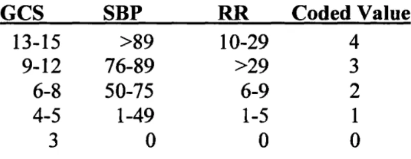
opening; verbal response and motor response) which formed an interval scale. The Triage Index was evaluated by Champion et al (1980) using a logistic regression model with a decision rule of 0.5 to determine the misclassification rate. The Triage Index was shortly amended to the Trauma Score (Champion, 1981). The Trauma Score (TS) also contained five physiological variables: respiratory rate; respiratory effort; systolic blood pressure; capillary refill and Glasgow Coma Scale. The Trauma Score was also evaluated using a logistic regression model. Misclassification rates and a less well known statistic called relative information gain* were used to assess the model’s goodness of fit. A further revision of the original Triage Index was published by Champion et al (1989) and the Trauma Score was amended to its current form:- the Revised Trauma Score.

* information gain E = 2P(1-P) - misclassification rate *relative information gain R = E/2P( 1 -P)

Section 3. TRISS and ASCOT Models.

The TRISS probability of survival trauma scoring model was developed by Champion et al (1981) using logistic regression. The model was developed originally using the Trauma Score (Champion, 1981). The Revised version of the Trauma Score was subsequently incorporated into the TRISS methodology (Champion, 1989).

One of the envisaged uses of the TRISS methodology was to identify unexpected trauma deaths and unexpected trauma survivors. An unexpected trauma death was defined as any patient who died whose probability of survival was > 0.5 (TRISS fallout).

(16)

An unexpected survivor was any patient who survived whose probability of survival was < 0.5. Karmy-Jones et al (1992) showed that TRISS unexpected outcomes resulted in 54% of cases being misclassified compared to peer review. Hill et al (1992) also prospectively evaluated TRISS fallout groups and found that they tended to over estimate potentially avoidable deaths especially in patients with severe head injuries. More recently Norris et al (2002) reviewed 270 patients categorised by TRISS as unexpected survivors. Only 10.7% were found to be clinically unexpected survivors following peer review. Despite the limitations of TRISS with respect to fall-out cases TRISS methodology still remains an invaluable tool upon which to base trauma audit.

Cayten et al (1991) identified some further limitations of TRISS methodology, the most important being the inability to account for multiple injuries in one body region. This limitation of the TRISS model led Champion et al (1990b) to develop an alternative anatomically based injury severity scoring system call the Anatomical Profile Score. The Anatomical Profile defines four components; A (head and spinal cord, AIS > 2), B (thorax and fi"ont of neck, AIS > 2), C (all other serious injuries, AIS >2), D (all injuries with AIS < 2). Component D although defined by the Anatomical Profile method is not utilised in any subsequent calculations. The component scores are calculated by taking the square root of the sum of all the AIS scores greater than 2 for that component. The square root value was used in the methodology because Champion et al (1990b) argue that this gives better representation to the most severe injury in each region, additional

(17)

injuries having a subliminal effect rather than a simple additive effect. The Anatomical Profile Score was subsequently incorporated into A Severity Characterisation of Trauma (abbreviated to;-ASCOT) model (Copes, 1990). The other variables in the logistic model being the individual coded values of the Revised Trauma Score:- Glasgow Coma Scale (G), systolic blood pressure (S), respiratory rate (R). The final variable in the model being age which is represented as a five component interval scale rather than a dichotomous variable as in TRISS.

The ASCOT model takes the

form:-K = form:-KG + form:-K1(G) + form:-K2(S) + form:-K3(R) + form:-K4(A) + form:-K5(B) +form:-K6(C) + K7(Age).

PS= l/l+e'^

It is important to note that the ASCOT method has four set-aside groups whose probability of survival is either extremely good or extremely poor; (1) AIS score = 6 and RTS = 0, (2) Maximum AIS score < 6 and RTS = 0, (3) AIS score 6 and RTS > 0, (4) Maximum AIS score = 1 or 2 and RTS > 0. These four set-aside groups were given a probability of survival based upon their survival rates obtained from the study data set and were not therefore used in further model development. The ASCOT and also new TRISS coefficients were developed from a data set 15,957 patients taken from the MTOS database. The two models (ASCOT and TRISS) were then evaluated on a second data set of 15,954 patients also derived from the MTOS database. The HL value for ASCOT and TRISS models were; ASCOT 24.8, TRISS (new coefficients) 43.9, TRISS (1986 MTOS coefficients) 45.6.

(18)

Markle et al (1992) undertook a comparative study of the TRISS model (using MTOS derived p coefficients) versus ASCOT (m coefficients were those derived by Copes et al {1990}) on a data set of 5,685 patients. Both models had p values for the HL statistic that were < 0.001 i.e. both appeared to be a poor fit. Hannan et al (1995a) compared ASCOT to TRISS using coefficients derived from the ITEC database. They found that the ASCOT model performed acceptably but that the TRISS model did not. Hou et al (1996) performed a comparative study of TRISS versus ASCOT on a data set of 5,672 cases. Their results were inconclusive. A further evaluation study of the ASCOT model was performed by Champion et al (1996), ASCOT being compared to TRISS using the 1986 MTOS P coefficients. There was no significant difference between the ASCOT and TRISS models using ROC analysis in either the blunt or penetrating subgroup of patients. The HL values for the ASCOT model were superior to the TRISS model for both the blunt and penetrating group. Osterwalder et al (2000) compared the predictive survival rates of TRISS and ASCOT with the observed survival rates. The predictive survival rates were not significantly different between the TRISS and ASCOT models. These authors argued on the basis of their findings that the additional data collection effort required for ASCOT compared to TRISS may not be justified.

Section 5. Additional Problems with the TRISS Model.

The original TRISS model used age as a dichotomous variable in the adult trauma group. Using a continuous variable in this way tends to result in either over prediction or under prediction of

(19)

survival. Since the inception of the TRISS model subsequent researchers have tended to use age as a continuous variable rather than as a dichotomous one. Demetriades et al (1998) found that using age as a dichotomous variable was an important cause for misclassifications in the TRISS fallout group. Al West et al (2000) used age as a quadratic spline (knots at 12, 25, and 65 years) in a logistic regression model which also included ICD-9 codes for anatomic injury, mechanism of injury and pre-existing disease. Two-way interaction terms for several combination of injuries were also included in the model. This model (HARM: Harborview Assessment for Risk of Mortality) was found to be superior to both TRISS and ASCOT using calibration and discrimination statistics.

Milzman et al (1992) found that pre-existing disease was an important independent risk factor for predicting death. The study involved a comparison of patients with and without pre-existing disease controlling for age and ISS. Sacco et al (1993) also found that pre-existing disease had a significant impact on survival. These authors however also showed that because the prevalence of pre-existing disease was relatively small in the trauma population (4.8%) institutional performance measures (Z and W values) were unlikely to be significantly affected. Other variables have been identified as potential independent risk factors for death in trauma patients e.g. falls (Hannan, 1995b; Demetriades, 1998), elevated blood lactate levels (Sauaia, 1994), blood pH (Milham, 1995) and a Systemic Inflammatory Response Syndrome* Score of 2 on admission (Napolitano, 2000).

’“SIRS score ranges from 1-4. One point is scored for each component present; fever or hypothermia, tachycardia, tachypnea and leukocytosis.

(20)

It has been be argued that death/survival is a crude outcome measure and this has led other investigators to use other outcome measures such as multiple organ failure (Roumen, 1993; Sauaia, 1994) and length of hospital stay (Clark, 1997). Multiple organ failure accounts for only a small proportion of trauma deaths (7%: Sauaia, 1995) and therefore is only applicable to a subgroup of trauma patients. Length of stay as an outcome variable has the draw back that it requires the exclusion of the subgroup of patients who die early (i.e. within 24 hours).

Section 5. New Injury Severity Score (NISS).

Osier et al (1997) suggested a simple solution to overcome one of the main limitations of ISS i.e. its inability to account for multiple injuries in one anatomical region. The modification consisted of summing the squares of the three highest AIS scores irrespective of anatomical region. The modification was named NISS (New Injury Severity Score) by the authors. NISS was evaluated on two independent data sets (Albuquerque data set n = 3,136 and Oregon data set n = 3,449) and a comparison was made with ISS. The study appeared to demonstrate the superiority of NISS over ISS using the HL statistic and ROC analysis. A comparative study of NISS versus ISS was performed by Brenneman et al (1998) on a data set of 2,328 patients. The two scoring systems were discrepant in 68% of cases. In the group with discrepant scores NISS was superior to ISS using ROC curve analysis (0.852 versus 0.799 p < 0.001). Moini et al (2000) performed a comparative study of TRISS versus NISS + RTS + Age on a data set of 2,662 patients. Using TRISS derived Z and W scores they suggested that TRISS was superior to NISS + RTS + Age. Neither logistic regression nor

(21)

neural networks were used to evaluate the two models. Balogh et al (2000) performed a study comparing NISS to ISS on a data set of 295 patients using post-injury multiple organ failure (MOF) as the outcome variable. They found that NISS was superior to ISS. The main limitation of this study was that is was performed on a very small data set.

Al West (2000a) performed a comparative study of four models (ISS, NISS, TRISS, NTRISS {NISS in lieu of ISS}) using the National Trauma Data bank of 52,566 cases. ISS was found to outperform NISS using measures of calibration (ISS HL: 134.4; NISS HL: 166.8) and discrimination (ISS ROC: 0.888; NISS ROC: 0.882; p = 0.0001). There was no significant difference in the ROC values (p = 0.039) between TRISS (0.956) and NTRISS (0.958). The HL values however showed a slight superiority of TRISS with new coefficients (HL: 186.2) over NTRISS (207.7). Grisoni et al (2001) evaluated ISS and NISS using ROC and HL analysis on 9,151 paediatric patients. They found that the predictive ability of NISS (using ROC) was not significantly superior to ISS, neither was the HL value. The majority of patients in the data set had mild injuries with an ISS < 9.

More recently Husum (2002) performed a comparative study of NISS versus ISS on a data set of 1,787 patients with penetrating war injuries. NISS was significantly better than ISS at predicting post-injury complications, however the accuracy of both tests was only moderate The authors of this study emphasised that the mortality in this study group was only 2.7%. At the present time the issue as to whether NISS is superior to ISS remains unresolved.

(22)

The differences between the two models do however appear to be partly dependent upon the composition of the data set.

Section 6. International Classification of Diseases

Injury Severity Score (ICISS).

The foundations of the ICD based scoring models are attributable to the work by Levy and co-workers (Levy, 1978; Goldberg, 1980; Levy, 1982; Goldberg, 1984). They conceptualised that the probability of survival could be calculated by multiplying the probability of survival for each injury using ICD based codes. They developed an Estimated Survival Probability Index (RES?) (Levy, 1978; Levy, 1982; Goldberg, 1984). This index failed to gain popularity at the time and was shortly superseded by the TRISS model.

Rutledge et al (1993) developed a data driven injury severity scoring model based upon the ICD-9 coding system. A mortality risk ratio (MRR) was developed for each ICD-9 code using the North Carolina database. The MRR model developed by Rutledge et al (1993) was based upon the premise that a given injury in isolation had the same value as a given injury in combination. This was a major weakness in the model design which probably led to it being abandoned.

The ICISS (International Classification of Disease-9 based Injury Severity Score) was developed by Osier et al (1996). The ICISS injury severity scoring model was based upon the ICD-9 discharge codes (800-959.9). A survival risk ratio (SRR) was determined for

(23)

each of the ICD-9 trauma injury codes using the North Carolina trauma database of 314,402. The SRR was calculated by dividing the number of times an ICD-9 code occurred in a surviving patient by the total number of times the ICD-9 code occurred in the data set. The ICISS was calculated for a given patient by the product of all their SRR’s. Using ROC analysis, outcome prediction was maximal when the five worst injuries (SRR’s) were used. However the outcome prediction was not reduced by using more injuries and so to avoid problems in injury selection all the SRR’s are used to calculate the ICISS. The ICISS was validated on the New Mexico database of 3,142 patients and the results were compared to ISS. ICISS was found to outperform ISS using ROC curve analysis and misclassification rates.

Two follow-up studies were subsequently published by Rutledge et al (1997, 1998). The first follow-up study (1997) showed that calibration of the ICISS model was superior to ISS using the HL test although the discrimination between the two models using ROC analysis was not significant. The results of the second follow-up study (Rutledge, 1998) also showed that the ICISS model was superior to the TRISS model. Hannan et al (1999) performed a comparative study comparing ICISS (ICD-9) with TRISS using the New York State trauma registry database. Although the ICISS outperformed both TRISS models the differences in results were less impressive than those obtained by Rutledge et al (1998).

(24)

Section 7. The Anatomical Profile Score.

Sacco et al (1999) performed a prospective study comparing five anatomical injury severity scales; ISS, ICISS, NISS, Anatomical Profile Score (APS{Copes et al, 1990}) and a modified version of the Anatomical Profile Score (mAP). The modified Anatomical Profile Score is composed of the three components (A,B,C) of the APS as previously described in section four of this chapter plus the maximum AIS value across all body regions. Their ICD mapped counterparts (ICD/ISS, ICD/NISS, ICD/APS, ICD/mAP) were also evaluated. The models were assessed using logistic regression on the PTOS database (derived from Peimsylvania’s 26 Level I trauma centres) using a data set of 60,574 patients. Coefficients were developed from half of the data set and model validation was performed on the other half. Using ROC analysis there was little difference between the models (ISS: 0.86, NISS: 0.86, ICISS: 0.88, APS: 0.87, mAP: 0.87). The HL statistic did however demonstrate large differences between the models (ISS: 384, NISS: 40, mAP: 29, APS: 70, ICISS: 370). The ICD mapped models showed no improvement in calibration or discrimination compared to then- respective counterparts.

Stephenson et al (2002) more recently performed a comparative study of five anatomic injury severity models: mapped (i.e. ICDMAP-90) modified-APS, mapped APS, mapped ISS, mapped NISS and ICISS. The study was performed on 349,409 cases derived from the New Zealand National Minimum Data Set. The ICISS model was found to have the largest concordance value (ROC=0.901). The mapped modified-APS had the best calibration using the HL statistic. Meredith et al (2002) also performed a

(25)

comparative study of nine scoring algorithms using a data set of 76,871 cases taken from the National Trauma Data Bank. The models used were modified-APS, ISS, NISS, maxAIS, mapped modified-APS, mapped ISS, mapped NISS, mapped maxAIS (i.e. the largest AIS score across all body regions) and ICISS. Model fit was assessed using ROC and HL statistics. Model validation was performed by 10-fold cross-validation, the final ROC and HL statistics being the mean of the cross validated results. The results from this study showed that the ICISS had the greatest discrimination (ROC=0.893 c.f. modified-APS ROC=0.887 {the second best score}). The modified-APS showed the best calibration (HL= 12.07 c.f. maxAIS HL= 19.47 {the second best score}). Interestingly ISS was found to outperform NISS with respect to calibration (HL:- NISS=48.34 HL:- ISS=33.25) and discrimination (ROC:- NISS=0.871 ISS=0.876).

Section 8. Conclusions

At the current time the issue of which is the ‘best’ anatomic injury model remains unresolved. Based upon recent studies by Meredith et al (2002) and Stephenson et al (2002) ICISS appears to have the better discrimination, whilst modified-APS appears to have the better calibration. Despite numerous studies it remains unclear as to whether NISS is superior to ISS. Differences between these two anatomic scoring models may be due more to the composition of the training and test data sets than any inherent superiority of one model over the other.

(26)

CHAPTER 3 PREPARATION OF THE LOS

ANGELES TRAUMA REGISTRY

DATA

Section 1. Composition

of the USC data set.

26

Section 2. Preparation of the USC revised data set.

3

1

Step 1. Placing data onto the SPSS spread sheet.

Step 2. Selection of variables for model building. Step 3. Deletion of paediatric cases.

Step 4. Deletion of missing variables. Step 5. Further refining of the data set.

Step 6. Deletion of cases with inaccuracies by variable.

Step 7. Identifying and deleting cases with group inaccuracies. Step 8. Preparation of the Mechanism of Injury variable.

Section 3. Composition

of the revised USC data set.

47

Section 4. Discussion.

56

(27)

Section 1: THE DATA SET

The USC data set was obtained from the department of Traumatology, Los Angeles County Hospital. This is the Level 1 trauma centre serving the whole of Los Angeles. The hospital is affiliated to the University of Southern California. The data set will be referred to as the USC data set.

Section 1.1 Composition of the USC data set

All cases entered into the trauma registry from the 1st January 1995 to the 31 December 1998 are included in the data set.

The following variables were included in the data

set:-Age; (years) The value is rounded off to a whole year (except when less than 12 months of age).

Mechanism of Injury Variable. There are two mechanism of injury variables: First mechanism of injury (MOIl) and second mechanism of injury (M0I2). The mechanism of injury codes contain a combination of epidemiology codes (e.g. work related WR) and actual mechanisms of injury codes (e.g. stab wound:- SW). These two types of codes may occur in either the first or second MOI group. MOIl is the main category. M0I2 is used when additional mechanism of injury data is available.

The codes for the mechanism of injury variable categories (MOIl and M0I2) are given

(28)

W = Versus Vehicle, subcategory of motorcycle /moped MM = Motorcycle/moped

OT = Other mechanism of injury PS = Passenger space intrusion

SA = Self inflicted wound, accidental SI = Self inflicted wound, intentional WR = Work related

WB = With blunt instrument, subcategory of assault

SF = Survivor of fatal accident, subcategory of enclosed vehicle SP = Sports injury

GS = Gunshot ST = Stabbing AS = Assault FA = Fall

TB = Thermal bum ES = Electric shock UN = Unknown

EV, EX, EJ, PB, TR, although often result in blunt trauma, penetrating injuries cannot be excluded.

EV = Enclosed vehicle EX = Extrication required EJ = Ejected fi*om vehicle

PB = Pedestrian/bike versus vehicle TR = Trauma arrest

(29)

SB = Seat belt. This is not strictly a mechanism of injury but is recorded in the M0I2 category when possible, in accidents when the victim is inside a vehicle.

HL = Helmet. Similarly this is not a mechanism of injury but is recorded in the MOI2 category when possible, in accidents when the victim is riding a motorbike or moped.

There are no mechanism of injuries which are restricted purely to MOIl or MOI2 although certain combinations are commonly seen e.g. TR (MOIl) and GS (M0I2). Approximately 50% of patients had a second mechanism of injury recorded.

The number of penetrating injuries in the first mechanism of injury category was 3030 (SI = 38, SA = 24, ST = 1667, GS = 1301). The number of cases with a penetrating mechanism of injury in the second mechanism of injury category was 2110 (SI = 125, SA = 20, ST = 126, GS = 1839).

In 120 cases a penetrating injury (SI, SA, ST, GS) was recorded in both first and second mechanism of injury categories. There were only two cases where a patient had both a stabbing injury (ST) and also a gun shot wound (GS). There were no cases where the same mechanism of injury code was recorded in both the first and second category. The total number of patients with a penetrating mechanism of injury recorded was therefore 5020 [(3030 +2110) -

120].

(30)

There is good evidence from the work by Champion et al (1990a) that patients with penetrating injuries have a lower predicted probability using TRISS because of the limitations of the ISS with regard to its constraints of including only one AIS per body region. Mechanism of injury was not used for modelling because it can only be represented as a dichotomous variable i.e. penetrating versus blunt. Dichotomous variables generally perform poorly in logistic regression models.

Other Variables

Abbreviated Injury Score; (abbreviated notation;- AIS).

Admission Systolic blood pressure (abbreviated notation:- SBP). Admission Glasgow Coma Scale (abbreviated notation:- GCS). Admission Respiratory Rate (abbreviated notation:- RR).

ISS:- Injury Severity Score calculated using ICD-9 conversion software.

HCISS:- Injury Severity Score. A hand calculated Injury Severity Score summing the square of the three highest Abbreviated Injury Scores (AIS) with the proviso that any individual body region can only be represented once.

Outcome (death or survival); coded as death = 0, survival = 1. Body region. The region was coded using AIS 85 classification:- Head/Neck=l, Face=2, Chest=3, Abdomen/Pelvis=4,

Extremities=5, Extemal=6.

A total of 13447 cases are in the data set for the period:- 01/01/1995-31/12/1998.

(31)

Number of cases recorded per year: 1995: - 3397, 1996:- 2901, 1997:-3167, 1998:- 3972.

Section 1.2: Individual Variables

Age: Patients of all ages are included in the USC data set. Number of missing cases = 13447 - 13443 = 4

AIS: Number of missing cases = 13447 - 13073 = 374 RR: Number of missing cases 13447 -12796 = 651

SBP: Number of missing cases 13447 - 12993 = 454

GCS: Number of missing cases 13447 - 12747 = 700

HCISS: Number of missing cases 13447 - 13283 = 164

ISS: Number of missing cases 13447 - 13069 = 378

Outcome: Number of missing cases 13447 - 13381 = 66

(32)

Section 2: Preparation of the Revised Data Set.

Step 1.

The data set was transferred from an Excel spreadsheet onto an SPSS spreadsheet for analysis.

Step 2. Selection of variables for the final data set.

The following variables were selected; HCISS, SBP, RR, GCS, coded Outcome and Age. HCISS was selected in preference to ICD-9 mapped ISS due to the inaccuracies which may occur during the conversion. The mechanism of injury variables (MOIl and MOI2) were also included in the revised data set so that the percentage of penetrating injuries and blunt injuries could be calculated. Blunt injury was coded 1, penetrating injury was coded 2, cases classified only by using epidemiology codes e.g. SP (sports injury) were coded 3.

Step 2.1 Coding of mechanism of injury variables.

Blunt injuries were coded 1. Penetrating injuries were coded 2.

Epidemiological coding e.g. WR (work related), SP (sports injury). AS (assaults) were coded 3.

Cases classified solely as UN (unknown) were coded 1. TR (trauma arrests) were coded 4.

Step 3. Deletion of Paediatric Cases.

Cases where the age of the patient was less than 16 years were deleted from the revised data set in view of the fact that paediatric

(33)

patients have different normal values for systolic blood pressure and respiratory rate depending upon age.

A total of 1100 cases were present where the patient’s age was found to be less than 16 years. No further analysis of these cases was performed. Deletion of cases with an age of 15 years or less left the revised data set with 12,347 cases.

Step 4. Deletion of Missing Variables.

The Hosmer Lemeshow statistic is one of the main goodness of fit tests used in logistic regression modelling. This test will be evaluated further in this thesis. The value of the HL test like several other goodness of fit tests (e.g. Copas, Deviance and Pearson) increases as the data set size increases. In order to evaluate these goodness of fit tests with different predictor variables it is a pre-requisite that there are no missing values from any of the variables which are to be used for model building. Deletion of cases with missing values using the variables previously mentioned resulted in the revised data set having 11,108 cases. The cases which had missing values from the mechanism of injury variables (MOIl and MOI2) were not deleted from the data set in view of the fact that it was not intended to use these two variables for model building. The deletion of missing variables was performed by pasting the data set into SAS. A short SAS program was then written using the statement; if variable = . then delete. The data set was then exported in excel format and transposed back into SPSS.

(34)

Step 5.1 Refining the Data Set

All patients admitted under the Department of Traumatology have

their injuries, demographic details and epidemiology recorded in

the trauma registry. Many patients are admitted for observation on

the basis of mechanism of injury criteria alone and therefore will

turn out to have minor injuries and an ISS of 1, 2 or 3. Inclusion of

such patients results in a large left hand skew to the distribution of

ISS values. Graph 1 shows this large left hand skew due to the

large number of minor injuries. Cases with an ISS of 1, 2 or 3

represent such minor injuries that any deaths that occur in this

group can only be explained by co-morbidity or by errors in

calculating or recording the ISS. For the latter two reasons all

HCISS cases less than 4 were deleted from the revised data set.

The deletion of all HCISS cases < 4 resulted in a revised data set of

7,364 cases.

Distribution of HCISS

4000

3000

3 2000

rrfMn I * ■ 1 n~Lr^» —n

.00 6.00 13.00 20.00 27.00 35.00 45.00 59.00 3.00 10.00 17.00 24.00 32.00 41.00 51.00 81.00

HCISS

(35)

Graph 1: The distribution of all HCISS cases demonstrates a strong left hand skew.

c

g

Distribution of HCISS

1400

1200

1000

600 400 200 0

4 00 11 00 18 00 25 00 33 00 42 00 54 00 8 00 14 00 21 00 29 00 36.00 48 00 66 00

HCISS

Graph 2: The distribution following deletion of all HCISS cases < 4 still leaves a strong left hand skew.

Step 5.2

A HCISS value of 81 represents an injury which is not classifiable,

these cases were deleted from the data set. 72 cases were identified

with an HCISS=81. The refined data set = 7,292 cases.

Step 5.3

Ten cases where HCISS= 75 and dl=l were found (table 1). All of

these cases were deleted. The refined data set = 7,282.

(36)

Case Summaries

ISS HCISS GCS SBP RR AGE DL NUM

1 75.00 75.00 14.00 72.00 28.00 39.00 1.00 1031.00 2 4.00 75.00 15.00 136.00 20.00 35.00 1.00 1034.00 3 1.00 75.00 15.00 136.00 24.00 46.00 1.00 1124.00 4 75.00 75.00 3.00 .00 .00 16.00 1.00 3823.00 5 75.00 75.00 4.00 .00 1.00 55.00 1.00 6814.00 6 75.00 75.00 15.00 137.00 38.00 18.00 1.00 7356.00 7 75.00 75.00 15.00 120.00 20.00 22.00 1.00 8122.00 8 75.00 75.00 3.00 121.00 1.00 19.00 1.00 8360.00 9 25.00 75.00 3.00 .00 1.00 20.00 1.00 9052.00 10 10.00 75.00 15.00 136.00 28.00 41.00 1.00 10492.00

Total N 10 10 10 10 10 10 10 10

a Limited to first 100 cases.

Table 1

Step 5.4

There have been no reported cases of patients surviving with an ISS of greater than 50 although the possibility of this remains as Trauma Units become more skilled at treating patients with severe injuries. Only one patient was found to have an ISS > 50 with an outcome = 1 (table 2). The values of the associated variables (i.e. all other variables within normal range) suggest that there was probably an error in recording the outcome variable. This case was deleted. The revised data set size = 7,281.

Case Summaries

GCS SBP RR HCISS AGE DL NUM ISS

1 Total N

15.00 1 136.00 1 20.00 1 59.00 1 20.00 1 1.00 1 1110.00 1 59.00 1 a Limited to first 100 cases.

Table 2

(37)

Step 6: Deletion of cases with inaccuracies by variable.

Inaccuracies in the variables can be determined in two ways. Firstly by identifying values which are outside the anticipated range for the physiological variable (i.e. systolic blood pressure, respiratory rate) or parameter (ISS or GCS). The second method of identifying inaccuracies is to compare the value of all the variables together and then to look for physiological inconsistencies.

Identification Of Values Outside The Normal Range.

Step 6.1 The GCS Variable.

Examination of the distribution of GCS values showed that some typographical errors had occurred with GCS values of greater than 15 being recorded. All GCS values greater than 15 were deleted from the data set (n=I8). The revised data set = 7,263 after deletion of GCS > 15. A single case was identified (table 3) where the GCS was recorded as less than 3. This case was deleted. The revised data set after deletion = 7,262.

Case Summarfes

ISS GCS SBP RR HCISS AGE DL NUM

1 Total N

9.00 1 2.00 1 146.00 1 18.00 1 4.00 1 25.00 1 1.00 1 1757.00 1 a Limited to first 100 cases.

Table 3

(38)

Step 6.2 Respiratory Rate Variable RR

A precise upper limit for respiratory rate is not clearly defined compared to the GCS. It is unlikely however that an adult patient could maintain ventilation with a rate above 60 breaths per minute. Examination of the distribution of all patients with a respiratory rate greater than 40 per minute is shown in table 4. This demonstrated that only two cases had a RR which was just over (i.e. defined as being less than 65) the cut-off value of 60 (number 44, RR=64 and number 45, RR=62). Using a cut-off value of sixty would not result in loss of a large number of borderline cases. All cases with a RR over 60 per minute were deleted (n=32). The revised data set = 7,230.

(39)

u> 00

S 8 8 8 8 8 8 8 8 8 8 8 8 8 8 8 8 8 8 8 8 8 8 8 8 8 8 S 8 8 8 8 8 8 8 8 8 8 S 8 8 8 8 8 8 8 8 8 8 8 8 8 8 8 8 8 8 8 8 8 8 8 8 8 8 8 8 8 8 8 8 8 8 8 8 8 8 8 8 8 8 8 8 8 8 8 8 8 8 8 8 8 8 8 8 8 8 8 8 8 8 8 8 8 8 8 8 8 8 8 8 8 8 8 8 8 8 8 8 8 8 8 8 8 8 8 8 8 8 8 8 8

u i u i u i c n u i o > - ^ c n u i u i c n o i c n ^ ( o a i a i ( o - ^ c n a < u i u i > c n ( A i ( 7 i o i ^ N > w v i u i w u i a i u i o i u i o > o i o a c < > u i t s j a i o n i n u i - » o i c n u a i u i c n a > c i i c i i ^ u i o u - ^ c n

8 8 8 8 8 8 8 8 8 8 8 8 8 8 8 8 8 8 8 8 8 8 8 8 8 8 8 8 8 8 8 8 8 8 8 8 8 8 8 8 8 8 8 8 8 8 8 8 8 8 8 8 8 8 8 8 8 8 8 8 8 8 8 8 8 8 8 8 8 8 8 8 8 8 8 8 8 8 8 8 8 8 8 8 8 8 8 8 8 8 8 8 8 8 8 8 8 8 8 8 8 8 8 8 8 8 8 8 8 8 8 8 8 8 8 8 8 8 8 8 8 8 8 8 8 8 8 8 8 8 8 8 8 8 8 8 8 8 8 8 8 8 8 8 8 8 8 8 8 8 8 8 8 8 8 8 8 8 8 8 8 8 8 8 8 8 8 8 8 8 8 8 8 8 8 8 8 8 8 8 8 8 8 8 8 8 8 8 8 8 8 8 8 8 8 8 8 8 8 8 ‘8 '8' 8 8 8 8 8 8 8 8 ' 8 8 8 8 8 8 8 8 8 8 8 8 8 8 8 8 8 8 8 8 8 8 8 8 8 8 8 8 8 8 8 8 8 8 8 8 8 8 8 8 8 8 8 8 8 8 8 8 8 8 8 8 8 8

8 8 8 8 8 8 8 8 8 8 8 8 8 8 8 8 8 8 8 8 8 8 8 8 8 8 8 8 8 8 8 8 8 8 8 8 8 8 8 8 8 8 8 8 8 8 8 8 8 8 8 8 8 8 8 8 8 8 8 8 8 8 8 8 8 8

_ ^ ^ ^ ^ ^ ^ J S S 8 2 2 2 8 S S î S 5 2 8 8 8 S S § S : : l 5 l S ; ; j S â 2 8 8 S 3 2 2 8 è è è 6 2 ± 2 2 8 K K S i 5 o . A N ,

(40)

Step 6.3 Systolic Blood Pressure Variable SBP

The upper limit of normal for systolic blood increases with age. The majority of patients attending emergency departments will have some elevation in their blood pressure due to 'stress'. The combination of these two makes an easily identifiable cut-off level between the upper limit of normal and an error in recording the SBP problematic. The cut-off point for systolic blood pressure was made at 250mmHg. Five patients had a systolic blood pressure over 250mmHg. The revised data set following the deletion of these five cases was 7,225.

Case Summariês

HCISS GCS SBP RR AGE DL NUM

1 26.00 3.00 999.00 1.00 19.00 .00 326.00

2 8.00 14.00 254.00 26.00 71.00 1.00 1624.00

3 9.00 15.00 256.00 32.00 52.00 1.00 5532.00

4 5.00 15.00 253.00 24.00 30.00 1.00 5745.00

5 30.00 7.00 252.00 1.00 46.00 1.00 1787.00

Total N 5 5 5 5 5 5 5

a-Limited to first 100 cases.

Table 5

Step 6.4: Age Variable.

No inaccuracies were noted with the recorded age values. All patients had an age of less than 100 years.

Step 7. Group Inaccuracies.

Inaccuracies in the data were also identified by examining the three physiological variables as a group.

(41)

Step 7.1

A case with a respiratory rate recorded as zero but with a GCS > 3 would be inconsistent and these cases were identified (table 6) and deleted. A patient could still have a relatively normal blood pressure for a brief period of time before progressing to cardio respiratory arrest. Cases with a recordable systolic blood pressure were therefore not deleted. 76 cases were deleted in total and the revised data set = 7,149.

Step 7.2

Examination of cases with a respiratory rate of less than 10 revealed some inconsistencies. A patient with a respiratory rate of between 1 and 5 would be expected to be unconscious; consistent with a GCS of 8 or less. All patients with a GCS of greater than 8 and a respiratory rate between 1 and 5 were identified (table 7) and deleted (n=37). The revised data set = 7,112.

(42)

Case Summaries

ISS HCISS GCS SBP RR AGE DL NUM

1 17.00 26.00 5.00 148.00 .00 19.00 .00 15.00

2 20.00 29.00 4.00 .00 .00 25.00 .00 523.00

3 17.00 17.00 5.00 155.00 .00 20.00 1.00 552.00

4 38.00 75.00 15.00 .00 .00 25.00 .00 766.00

5 50.00 43.00 7.00 82.00 .00 25.00 .00 778.00

6 26.00 26.00 7.00 116.00 .00 17.00 .00 938.00

7 16.00 25.00 5.00 142.00 .00 18.00 .00 1002.00

8 43.00 43.00 7.00 70.00 .00 58.00 .00 1063.00

9 57.00 48.00 4.00 50.00 .00 36.00 .00 1077.00

10 10.00 10.00 7.00 100.00 .00 25.00 1.00 1114.00

11 16.00 25.00 5.00 96.00 .00 20.00 .00 1196.00

12 13.00 13.00 7.00 134.00 .00 26.00 1.00 1218.00

13 17.00 16.00 8.00 86.00 .00 36.00 .00 1675.00

14 20.00 24.00 4.00 116.00 .00 30.00 1.00 1890.00

15 16.00 9.00 9.00 211.00 .00 20.00 1.00 1891.00

16 25.00 16.00 15.00 120.00 .00 27.00 1.00 1906.00

17 5.00 41.00 6.00 90.00 .00 16.00 .00 1971.00

18 16.00 25.00 6.00 124.00 .00 17.00 .00 2100.00

19 16.00 16.00 7.00 132.00 .00 35.00 1.00 2132.00

20 16.00 16.00 6.00 166.00 .00 20.00 1.00 2153.00

21 26.00 21.00 10.00 70.00 .00 35.00 .00 2214.00

22 16.00 25.00 4.00 130.00 .00 20.00 .00 2246.00

23 26.00 26.00 4.00 64.00 .00 73.00 .00 2282.00

24 41.00 50.00 9.00 80.00 .00 30.00 .00 2319.00

25 38.00 38.00 7.00 116.00 .00 22.00 1.00 2393.00

26 25.00 25.00 5.00 94.00 .00 26.00 .00 2434.00

27 16.00 26.00 5.00 193.00 .00 34.00 .00 2690.00

28 35.00 35.00 7.00 181.00 .00 71.00 .00 2812.00

29 22.00 17.00 6.00 148.00 .00 23.00 1.00 2879.00

30 16.00 16.00 15.00 165.00 .00 50.00 1.00 2935.00

31 26.00 17.00 6.00 95.00 .00 19.00 .00 2997.00

32 9.00 9.00 6.00 105.00 .00 40.00 1.00 3201.00

33 26.00 26.00 5.00 102.00 .00 19.00 .00 3261.00

34 16.00 25.00 11.00 213.00 .00 23.00 .00 3476.00

35 16.00 16.00 4.00 138.00 .00 53.00 1.00 3525.00

36 25.00 25.00 5.00 181.00 .00 21.00 1.00 3631.00

37 26.00 25.00 6.00 142.00 .00 47.00 1.00 3884.00

38 9.00 9.00 9.00 114.00 .00 18.00 1.00 3959.00

39 29.00 29.00 5.00 88.00 .00 30.00 1.00 4122.00

40 22.00 22.00 8.00 120.00 .00 21.00 1.00 4128.00

41 11.00 11.00 14.00 160.00 .00 70.00 1.00 4216.00

42 29.00 25.00 7.00 73.00 .00 34.00 .00 4299.00

43 4.00 4.00 8.00 179.00 .00 16.00 1.00 4357.00

44 9.00 9.00 11.00 82.00 .00 30.00 1.00 4486.00

45 14.00 14.00 8.00 145.00 .00 43.00 1.00 4745.00

46 29.00 24.00 7.00 92.00 .00 38.00 1.00 4754.00

47 26.00 35.00 8.00 137.00 .00 20.00 1.00 4852.00

48 10.00 10.00 12.00 216.00 .00 45.00 1.00 4904.00

49 26.00 26.00 5.00 106.00 .00 16.00 .00 4970.00

50 21.00 21.00 10.00 156.00 .00 34.00 1.00 5009.00

51 30.00 30.00 6.00 101.00 .00 41.00 .00 5066.00

52 4.00 4.00 15.00 150.00 .00 36.00 1.00 5108.00

53 26.00 5.00 4.00 112.00 .00 23.00 1.00 5138.00

54 26.00 26.00 6.00 112.00 .00 26.00 .00 5238.00

55 17.00 16.00 15.00 104.00 .00 20.00 .00 5402.00

56 13.00 8.00 5.00 117.00 .00 26.00 1.00 5421.00

57 9.00 9.00 4.00 76.00 .00 20.00 1.00 5513.00

58 75.00 75 00 6.00 .00 .00 25.00 .00 5629.00

59 34.00 43.00 6.00 138.00 .00 19.00 1.00 5729.00

60 75.00 75.00 6.00 .00 .00 29.00 .00 5734.00

61 41.00 50.00 13.00 70.00 .00 67.00 .00 5927.00

62 17.00 17.00 6.00 60.00 .00 36.00 1.00 6043.00

63 17.00 16.00 4.00 157.00 .00 30.00 1.00 6052.00

64 25.00 34.00 6.00 193.00 .00 27.00 1.00 6053.00

65 20.00 20.00 15.00 120.00 .00 52.00 1.00 6097.00

66 26.00 26.00 7.00 112.00 .00 36.00 .00 6120.00

67 26.00 26.00 6.00 108.00 .00 16.00 .00 6165.00

68 29.00 29.00 10.00 66.00 .00 82.00 .00 6179.00

69 17.00 12.00 6.00 .00 .00 35.00 1.00 6190.00

70 16.00 16.00 15.00 147.00 .00 21.00 1.00 6726.00

71 34.00 34.00 15.00 .00 .00 39.00 1.00 6750.00

72 16.00 16.00 6.00 .00 .00 20.00 .00 7084.00

73 4.00 4.00 15.00 122.00 .00 35.00 1.00 9782.00

74 26.00 17.00 14.00 192.00 .00 65.00 .00 11105.00

75 9.00 9.00 15.00 144.00 .00 20.00 1.00 12801.00

76 34.00 34.00 9.00 58.00 .00 36.00 .00 13193.00

Total N 76 76 76 76 76 76 76 76

=' Limited to first 100 ca se s.

Table 6

(43)

Case Summaries

HCISS GCS SBP RR AGE NUM DS

1 26.00 12.00 172.00 1.00 19.00 .00 454.00

2 10.00 11.00 .00 4.00 17.00 .00 3551.00

3 9.00 15.00 118.00 2.00 31.00 1.00 4134.00

4 9.00 15.00 85.00 1.00 31.00 1.00 4281.00

5 16.00 10.00 97.00 1.00 47.00 .00 5770.00

6 41.00 15.00 72.00 1.00 30.00 .00 5876.00

7 29.00 10.00 105.00 1.00 35.00 1.00 6017.00

8 20.00 10.00 130.00 1.00 24.00 1.00 6090.00

9 18.00 13.00 104.00 1.00 31.00 1.00 6198.00

10 25.00 12.00 54.00 1.00 46.00 1.00 6270.00

11 5.00 15.00 142.00 1.00 22.00 1.00 6487.00

12 33.00 9.00 71.00 1.00 59.00 .00 6696.00

13 9.00 9.00 85.00 1.00 38.00 1.00 6850.00

14 29.00 10.00 156.00 1.00 55.00 1.00 7133.00

15 20.00 11.00 110.00 1.00 28.00 1.00 7264.00

16 14.00 15.00 136.00 1.00 30.00 1.00 7287.00

17 33.00 15.00 80.00 1.00 19.00 .00 7364.00

18 33.00 11.00 121.00 1.00 40.00 1.00 7579.00

19 29.00 12.00 .00 1.00 35.00 .00 8045.00

20 21.00 9.00 153.00 1.00 21.00 .00 8149.00

21 9.00 15.00 85.00 1.00 48.00 1.00 8173.00

22 22.00 11.00 .00 1.00 65.00 .00 8332.00

23 14.00 14.00 128.00 1.00 30.00 1.00 9453.00

24 18.00 15.00 .00 1.00 17.00 1.00 9831.00

25 41.00 15.00 152.00 1.00 24.00 .00 9880.00

26 30.00 11.00 .00 1.00 54.00 .00 10202.00

27 36.00 12.00 134.00 1.00 50.00 .00 10206.00

28 8.00 9.00 169.00 1.00 18.00 1.00 10831.00

29 75.00 15.00 .00 1.00 38.00 .00 11162.00

30 16.00 15.00 .00 4.00 25.00 .00 11202.00

31 17.00 10.00 164.00 1.00 35.00 1.00 11455.00

32 25.00 15.00 .00 1.00 20.00 .00 11660.00

33 17.00 15.00 .00 1.00 29.00 .00 11697.00

34 26.00 10.00 185.00 1.00 75.00 .00 11744.00

35 50.00 14.00 .00 1.00 35.00 .00 12225.00

36 22.00 13.00 108.00 1.00 18.00 .00 12341.00

37 25.00 15.00 .00 1.00 19.00 .00 12958.00

Total N 37 37 37 37 37 37 37

a Limited to first 100 cases.

Table 7

(44)

Step 7.3

Patients with a systolic blood pressure equal to zero are clinically dead and therefore would have a GCS of 3. Cases with a SBP = 0 and a GCS > 3 were identified and deleted (table 8). The revised data set = 7,077.

Case Summariel

ISS HCISS GCS SBP RR AGE DL NUM

1 25.00 26.00 11.00 .00 16.00 32.00 .00 1.00

2 16.00 25.00 4.00 .00 1.00 25.00 .00 4.00

3 34.00 41.00 4.00 .00 1.00 30.00 .00 201.00

4 25.00 25.00 12.00 .00 16.00 39.00 1.00 338.00 5 32.00 32.00 14.00 .00 30.00 21.00 1.00 1262.00 6 16.00 16.00 13.00 .00 32.00 21.00 .00 2741.00 7 18.00 18.00 12.00 .00 16.00 27.00 1.00 2795.00 8 4.00 9.00 14.00 .00 32.00 28.00 1.00 2906.00 9 9.00 9.00 9.00 .00 24.00 16.00 1.00 2968.00 10 25.00 18.00 14.00 .00 24.00 18.00 .00 3130.00 11 26.00 26.00 11.00 .00 10.00 25.00 .00 4500.00 12 17.00 26.00 14.00 .00 22.00 44.00 .00 4643.00 13 14.00 17.00 15.00 .00 16.00 43.00 1.00 4764.00 14 43.00 43.00 13.00 .00 28.00 20.00 .00 6440.00 15 59.00 50.00 12.00 .00 24.00 32.00 .00 6914.00 16 10.00 10.00 15.00 .00 20.00 18.00 1.00 6996.00 17 9.00 9.00 15.00 .00 22.00 17.00 1.00 7094.00 18 17.00 17.00 10.00 .00 24.00 20.00 1.00 7134.00 19 17.00 17.00 15.00 .00 32.00 30.00 1.00 8046.00 20 17.00 17.00 14.00 .00 18.00 24.00 .00 8630.00 21 17.00 17.00 7.00 .00 1.00 31.00 .00 8661.00 22 16.00 16.00 8.00 .00 14.00 22.00 1.00 8709.00 23 51.00 51.00 15.00 .00 24.00 17.00 .00 9047.00 24 51.00 51.00 6.00 .00 1.00 71.00 .00 9381.00 25 11.00 11.00 15.00 .00 16.00 64.00 1.00 9773.00 26 14.00 14.00 15.00 .00 20.00 17.00 1.00 9810.00 27 26.00 26.00 7.00 .00 1.00 17.00 .00 10369.00 28 13.00 13.00 15.00 .00 20.00 20.00 1.00 10646.00 29 25.00 25.00 7.00 .00 1.00 18.00 .00 11554.00 30 30.00 30.00 8.00 .00 20.00 24.00 1.00 11785.00 31 16.00 9.00 15.00 .00 24.00 25.00 1.00 12290.00 32 9.00 9.00 15.00 .00 24.00 19.00 .00 12507.00 33 18.00 18.00 7.00 .00 24.00 22.00 1.00 12564.00 34 14.00 14.00 15.00 .00 24.00 25.00 1.00 13014.00 35 16.00 9.00 15.00 .00 24.00 27.00 1.00 13258.00

Total N 35 35 35 35 35 35 35 35

a. Limited to first 100 cases.

Table 8

(45)

Step 7.4

Patients with a systolic blood pressure less than 50mmHg would be expected to have a depressed level of consciousness with a GCS of < 15. Cases with a SBP < 50 and a GCS = 1 5 were identified (table 9) and deleted. The revised data set = 7,069.

Case Summaries

HCISS GCS SBP RR AGE NUM DS

1 10.00 15.00 28.00 28.00 31.00 1.00 358.00

2 25.00 15.00 20.00 34.00 30.00 1.00 1363.00

3 19.00 15.00 40.00 28.00 17.00 .00 2485.00

4 19.00 15.00 40.00 44.00 22.00 1.00 5051.00

5 35.00 15.00 40.00 36.00 18.00 .00 5395.00

6 35.00 15.00 48.00 36.00 17.00 .00 5655.00

7 20.00 15.00 41.00 36.00 40.00 1.00 7240.00

8 25.00 15.00 48.00 40.00 45.00 1.00 11483.00

Total N 8 8 8 8 8 8 8

a Limited to first 100 cases.

Table 9

Step 8.

Further Preparation of the Mechanism of Injury Variables

Step 8.1

1,010 cases were recoded as value 4 (traumatic arrest) in the MOIl variable group. 1,008 of these cases had a corresponding recoded value of 2 in the M0I2 variable group and the final two cases in the MOI2 cell were blank. All of the cases except for the 2 blank cells (case numbers 8820 and 9776) were recoded 2 in a revised mechanism of injury variable group (MOB). The cases with the blank second cell were recoded as 3 in the MOB group.

(46)

Step 8.2

Fifteen cases were found to have a value of 1 (blunt trauma) in the MOIl group and a value of 2 (penetrating trauma) in the M0I2 group (table 10). No changes were made and the MOD variable was coded as 1.

Case Summartei

HCISS GCS SB P RR AGE DL NUM MOIl MOI2 MOIl REV

m oil =1 an d mol2 =2 (FILTER)

1 0.00 15.00 134.00 18.00 34.00 1.00 121.00 1.00 2.00 1.00 S elected

2 4.00 15.00 116.00 18.00 34.00 1.00 2078.00 1.00 2.00 1.00 S elected

3 5.00 3.00 162.00 1.00 19.00 1.00 5922.00 1.00 2.00 1.00 S elected

4 16.00 3.00 136.00 1.00 40.00 1.00 6550.00 1.00 2.00 1.00 Selected

5 5.00 10.00 131.00 20.00 33.00 1.00 6705.00 1.00 2.00 1.00 S elected

6 26.00 6.00 108.00 14.00 25.00 .00 7013.00 1.00 2.00 1.00 Selected

7 24.00 15.00 124.00 12.00 23.00 1.00 8021.00 1.00 2.00 1.00 S elected

8 4.00 15.00 128.00 20.00 31.00 1.00 8387.00 1.00 2.00 1.00 S elected

9 5.00 14.00 168.00 22.00 33.00 1.00 9315.00 1.00 2.00 1.00 S elected

10 8.00 15.00 155.00 26.00 40.00 1.00 10117.00 1.00 2.00 1.00 S elected

11 10.00 7.00 141.00 1.00 33.00 1.00 10892.00 1.00 2.00 1.00 Selected

12 4.00 15.00 103.00 18.00 40.00 1.00 11249.00 1.00 2.00 1.00 S elected

13 10.00 15.00 112.00 20.00 19.00 1.00 12807.00 1.00 2.00 1.00 S elected

14 5.00 6.00 133.00 24.00 38.00 1.00 12808.00 1.00 2.00 1.00 S elected

15 5.00 15.00 133.00 18.00 21.00 1.00 12819.00 1.00 2.00 1.00 S elected

Total N 15 15 15 15 15 15 15 15 15 15 15

3 Limited to first 100 c a se s .

Table 10

Step 8.3

Twenty cases were found to have a value of 2 in the MOIl group and a value 1 in the MOI2 group. These results are shown in table 11 (page 46). No changes were made and the MOD variable was coded as 2.

(47)

Case Summailei

HCISS G C S SB P RR AGE DL NUM MOIl MOI2 MOMREV

m oil =2 a n d moi2

= 1 (FILTER)

1 9.00 15.00 106.00 18.00 50.00 1.00 68 7 .00 2 .00 1.00 2 .0 0 S e lec te d

2 4.00 15.00 102.00 20.00 19.00 1.00 789.00 2.00 1.00 2.00 S e lec te d

3 14.00 15.00 142.00 16.00 50.00 1.00 1193.00 2.00 1.00 2.00 S e lec te d

4 6.00 15.00 152.00 28.00 18.00 1.00 1212.00 2.00 1.00 2.00 S e lec te d

5 50.00 11.00 68.00 24.00 42.00 .00 1334.00 2 .00 1.00 2.00 S e lec te d

6 20.00 3.00 120.00 6.00 19.00 1.00 1359.00 2.00 1.00 2.00 S e lec te d

7 5.00 15.00 138.00 20.00 18.00 1.00 2 504.00 2.00 1.00 2.00 S e lec te d

8 9.00 15.00 131.00 20.00 23.00 1.00 27 4 0 .0 0 2.00 1.00 2.00 S e lec te d

9 9.00 15.00 145.00 20.00 28.00 1.00 4 6 1 3 .00 2.00 1.00 2.00 S e lec te d

10 75.00 3.00 .00 .00 46.00 .00 6 0 0 4 .0 0 2.00 1.00 2 .0 0 S e lec te d

11 19.00 14.00 121.00 10.00 46.00 .00 7 202.00 2.00 1.00 2 .0 0 S e lec te d

12 5.00 4.00 142.00 18.00 28.00 1.00 94 2 9 .00 2.00 1.00 2.00 S e lec te d

13 36.00 14.00 140.00 24.00 30.00 1.00 95 5 3 .0 0 2.00 1.00 2.0 0 S e lec te d

14 25.00 3.00 164.00 20.0 0 19.00 .00 10655.00 2.00 1.00 2.0 0 S e lec te d

15 4.00 15.00 158.00 28.00 29.00 1.00 10899.00 2.00 1.00 2.0 0 S e lec te d

16 5.00 13.00 159.00 24.00 30.00 1.00 11168.00 2.00 1.00 2.0 0 S e lec te d

17 21.00 3.00 .00 1.00 36.00 .00 12105.00 2.00 1.00 2.0 0 S e lec te d

18 8.00 15.00 169.00 24.00 34.00 1.00 12333.00 2.00 1.00 2 .0 0 S e lec te d

19 4.00 15.00 133.00 22.00 36.00 1.00 12397.00 2.00 1.00 2.00 S e lec te d

20 12.00 15.00 108.00 22.00 38.00 1.00 12491.00 2.00 1.00 2.0 0 S e lec te d

Total N 20 20 20 20 2 0 20 20 20 20 20 20

a Limited to first 100 c a se s .

Table 11

Step 8.4

95 cases were found to have a value of 3 in the MOIl group and a value of 1 in the MOI2 group. All of these cases were recoded as 1 in the M0I3 variable group.

The MOD variable was created by combining data from the MOIl and MOI2 variables. The recoding was performed using a SAS program (shown below) after pasting the SPSS data set onto the SAS window. The data set was then exported and converted back into an SPSS data file.

SAS program used for creating the MOD variable.

DATA USCFINAL;

INPUT ISS HCISS GCS SBP RR AGE NUM DS m oil moi2 moi3; IF moil = 3 and moi2 = 1 then moi3 = 1;

IF moil = 3 and moi2 = 2 then moi3 = 2; IF moil = 3 and moi2 = . then moi3 = 3; IF moil = 3 and moi2 = 4 then moi3 = 3; IF moil = 1 and moi2 = 2 then moi3 = 1; IF moil = 1 and moi2 = . then moi3 = 1;

(48)

IF m oil = 1 and mol2 = 3 then moi3 = 1; IF moi 1 = I and moi2 = 4 then moi3 = 1 ; IF moil = 2 and moi2 = 1 then moi3 = 2; IF moil = 2 and moi2 = . then moi3 = 2; IF moil = 2 and moi2 = 3 then moi3 = 2; IF moil = 2 and moi2 = 4 then moi3 = 2; IF moil = 4 and moi2 = 2 then moi3 = 2; IF moil = 4 and moi2 = . then moi3 = 3; DATALINES;

RUN;

Section 2: Composition of the Revised Data Set.

Final number of cases in the revised data set = 7,069.

1. The Revised Mechanism of Injury Variable (MOI3)

Number of blunt trauma cases = 4,172

(fifteen of these cases also had a penetrating injury). Number of deaths in the blunt trauma group = 398

Survival rate in the blunt group = 90.5%

Number of penetrating trauma cases= 2,483 (20 of these cases also had a blunt injury).

Number of deaths in the penetrating trauma group = 481 Survival rate in the penetrating group = 80.6%

Number of cases unclassifiable = 396

Number of deaths in the unclassifiable group =13 Survival rate in the unclassifiable group = 96.7%.

Number of cases where data was not recorded in either the MOIl or M0I2 cell = 18. There was one death in this subgroup.

Survival rate = 94.4%.

(49)

The A ge V ariable

The Age distribution in the revised data set is shown in

Graph 3 below.

Distribution of Age Variable

4 0 0

3 0 0

3 200 100

Botta

1 6 0 0 2 6 .0 0 3 6 .0 0 4 6 0 0 5 6 .0 0 6 6 .0 0 7 6 .0 0 8 6 .0 0 9 9 .0 0 2 1 .0 0 31 0 0 4 1 .0 0 5 1 .0 0 6 1 .0 0 7 1 .0 0 8 1 .0 0 9 1 .0 0

AGE

Graph 3

The mean Age and standard deviation is shown in Table 12 below.

Descriptive Statistics

N Minimum Maximum Mean Std. Deviation AGE

Valid N (listwise)

7069 7069

16.00 99.00 35.3334 15.78480

Table 12

Trauma scoring models using logistic regression.