Non-linear optical response in disordered 2D materials
SimãoM. João2,∗ and JoãoM. Viana P. Lopes2,
1Centro de Física das Universidades do Minho e Porto, Universidade do Porto, 4169-007, Porto, Portugal. Departamento de Física e Astronomia, Faculdade de Ciências da Univer-sidade do Porto.
Abstract.Using KITE [1], a quantum transport software developed by ourselves, we explore the effect of disorder in the second-order con-ductivity, aiming to reproduce mesoscopic samples under more realistic models of disorder. This work will be concerned about our most recent results with KITE. We will showcase and examine how different mod-els of disorder affect the same system, experimenting with Anderson disorder and vacancies in gapped Graphene.
1 Introduction
Two-dimensional materials are a topic of great interest in the realm of nonlinear optics because they possess some of the strongest nonlinear optical responses to light. The bulk of the theoretical work developed to understand the nonlinear optical response of these materials [2–5] is concerned with translational-invariant systems, where disorder may be added perturbatively. In our work, we extend the work of Passos et al [6, 7] by implementing the velocity gauge methodology within the Keldysh formalism [8]. We developed a general perturbation procedure to deal with non-interacting fermion systems at finite temperature coupled to a time-dependent external electric field. We express the formula for the n-th order optical conductivity in terms of a trace, reflecting the fact that translation invariance was not needed for its derivation.
These expressions gain particular utility when used in the real-space basis, for then disorder may be introduced non-perturbatively and studied in, for example, tight-binding models. This includes Anderson disorder and any kind of structural disorder such as adatoms, vacancies and defects. This generality also allows one to study the effect of a magnetic field (which, through a Peierls phase, breaks translation symmetry on its own) in disordered systems.
Spectral methods such as the Kernel Polynomial Method (KPM) [9] become a very powerful tool to evaluate these traces, which, coupled with these formulas, enable the computation of the second-order response of large (106 atoms) disordered systems with a resolution of10meV [8]. These formulas, up to second order, are implemented in KITE, an open-source software tailored for scalable and efficient quantum transport simulations [1].
In the first part of this proceeding, we start by presenting the expressions obtained through the Keldysh framework [10]. Then, after a brief explanation on KPM we use
this framework to explore different models of disorder in gapped Graphene (GG), one of the simplest models for which we can find a second-order response to an external electric field. Since we are only interested in the intrinsic nonlinear optical response of the material, we are ignoring possible excitonic effects. Although we present GG specifically, KITE is able to calculate the transport properties of a very broad range of materials.
2 Nonlinear optical conductivity with the Keldysh formalism
Using the Keldysh formalism [10], we were able to obtain closed-form expressions for the general n-th order optical conductivity [8]. We only show the formulas up to second-order because the higher-order ones are too computationally expensive to be of practical use. The formulas for the first and second order conductivities obtained are, respectively,σαβ(ω) = ie 2 Ωω
ˆ ∞
−∞
df()Trˆhαβδ(−H0) (1)
+1
hˆαgR(/+ω) ˆhβδ(−H0) +
1
ˆhαδ(−H0) ˆhβgA(/−ω)
and
σαβγ(ω1, ω2) = 1 Ω
e3
ω1ω2 ˆ ∞
−∞
df()Tr 1
2hˆ αβγδ(
−H) (2)
+1
ˆhαβδ(−H)ˆhγgA(/−ω2) +
1
hˆαβgR(/+ω2) ˆhγδ(−H)
+ 1 2ˆh
αgR(/+ω
1+ω2) ˆhβγδ(−H) + 1 2ˆh
αδ(
−H)ˆhβγgA(/−ω1−ω2) +1
2ˆh
αgR(/+ω
1+ω2) ˆhβgR(/+ω2) ˆhγδ(−H) +1
2ˆh
αgR(/+ω1) ˆhβδ(
−H)ˆhγgA(/−ω2)
+1
2ˆh
αδ(
−H)ˆhβgA(/−ω1) ˆhγgA(/−ω1−ω2)
where ˆhα1···αn = 1
(i)n[ˆrα1,[· · ·[ˆrαn, H0]]], rˆis the position operator and gA,R are the advanced and retarded Green’s functions, respectively. If the system presents translation invariance and ak-space basis is used, we recover the known formulas for
the nonlinear optical conductivity derived through the density matrix formalism or Kubo’s formalism [6, 7]. A phenomenological broadening parameter0+
→γis added by hand in the Green’s functions to mimic the effect of inelastic scattering. In some cases, for pure systems, the conductivity may be infinite, which stems from the fact that there is no dissipation mechanism. Real systems exhibit some disorder, and to reflect this, the abovementioned phenomenological parameterγis added. Ideally, one should use real disorder, but this would break translation invariance. This will be the topic for the next sections.
this framework to explore different models of disorder in gapped Graphene (GG), one of the simplest models for which we can find a second-order response to an external electric field. Since we are only interested in the intrinsic nonlinear optical response of the material, we are ignoring possible excitonic effects. Although we present GG specifically, KITE is able to calculate the transport properties of a very broad range of materials.
2 Nonlinear optical conductivity with the Keldysh formalism
Using the Keldysh formalism [10], we were able to obtain closed-form expressions for the general n-th order optical conductivity [8]. We only show the formulas up to second-order because the higher-order ones are too computationally expensive to be of practical use. The formulas for the first and second order conductivities obtained are, respectively,σαβ(ω) = ie 2 Ωω
ˆ ∞
−∞
df()Trˆhαβδ(−H0) (1)
+1
ˆhαgR(/+ω) ˆhβδ(−H0) +
1
ˆhαδ(−H0) ˆhβgA(/−ω)
and
σαβγ(ω1, ω2) = 1 Ω
e3
ω1ω2 ˆ ∞
−∞
df()Tr 1
2ˆh αβγδ(
−H) (2)
+1
ˆhαβδ(−H)ˆhγgA(/−ω2) +
1
ˆhαβgR(/+ω2) ˆhγδ(−H)
+ 1 2ˆh
αgR(/+ω
1+ω2) ˆhβγδ(−H) + 1 2hˆ
αδ(
−H)ˆhβγgA(/−ω1−ω2) + 1
2hˆ
αgR(/+ω
1+ω2) ˆhβgR(/+ω2) ˆhγδ(−H) +1
2hˆ
αgR(/+ω1) ˆhβδ(
−H)ˆhγgA(/−ω2)
+1
2ˆh
αδ(
−H)ˆhβgA(/−ω1) ˆhγgA(/−ω1−ω2)
where ˆhα1···αn = 1
(i)n[ˆrα1,[· · ·[ˆrαn, H0]]], rˆis the position operator and gA,R are the advanced and retarded Green’s functions, respectively. If the system presents translation invariance and ak-space basis is used, we recover the known formulas for
the nonlinear optical conductivity derived through the density matrix formalism or Kubo’s formalism [6, 7]. A phenomenological broadening parameter0+
→γis added by hand in the Green’s functions to mimic the effect of inelastic scattering. In some cases, for pure systems, the conductivity may be infinite, which stems from the fact that there is no dissipation mechanism. Real systems exhibit some disorder, and to reflect this, the abovementioned phenomenological parameterγis added. Ideally, one should use real disorder, but this would break translation invariance. This will be the topic for the next sections.
Symmetry may cause some of these terms to be zero. In fact, due to centrosymme-try, Graphene displays no second-order response. GG does not have this symmetry
a1
a2
𝛿𝛿2
𝛿𝛿3 𝛿𝛿1
B A a1 a2 𝛿𝛿2 𝛿𝛿3 𝛿𝛿1 B A
a)
b)
x yFigure 1. Primitive vectors and atomic basis used in GG (a) and in the related model where one of the sublattices is displaced with respect to the other (b). The B sublattice is displaced by−δ2/2.
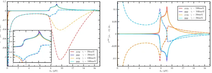
Figure 2. Photogalvanic effect in dGG (left) and GG (right). The gap is∆ = 7.78 eV. Lattice size: L= 2048, Fermi energyεF = 0eV. The solid curves represent the real part of the conductivity and the dashed curves the imaginary part.
and therefore has a second-order response. The photogalvanic effect in GG [11] is expected to diverge in the limit γ → 0+ as discussed in the previous paragraph. However, GG still has C3 rotational symmetry and three reflection axis, and these are in the origin of the cancellation of the terms in eq. 2 responsible for making the conductivity diverge.
To check this, we used the k-space basis to perform the calculations for two
dif-ferent values ofγ in GG and in another model with less symmetry, which we denote by ’displaced Gapped Graphene’ (dGG). This somewhat artificial model is the same as GG, but sublattice B is displaced by −δ2/2 with respect to sublattice A (see fig. 1), while maintaining the same hopping integrals between neighbours. Therefore, the velocity operator is modified but the Hamiltonian is not. In fig. 2, we see that γ controls the sharpness of the curves in GG, but has otherwise no qualitative effect on the conductivity. In dGG, for thexxy conductivity tensor, the symmetry responsible for making the conductivity diverge is not present, and a clear dependence onγexists in the imaginary part of the conductivity. For most practical applications, however, this is not problematic since only the real part of the conductivity is relevant.
3 The Kernel Polynomial Method
In order to compute the traces in eqs. 1 and 2 we resort to a Stochastic Trace Eval-uation (STE) and the Kernel Polynomial Method (KPM)[9]. Let |ξ = iξi|Ri be a vector with random numbers ξi, taken from a distribution X, assigned to each lattice siteRi and· · · denote the average with respect to that distribution. Then, imposing ξ∗
iξj = δij on the distribution, we get ξ|A|ξ = Tr(A). Due to the self-averaging properties of this procedure, usually only one random vector is needed. The functions of the Hamiltonian appearing in eqs. 1 and 2 have no immediate rep-resentation in a real-space basis, so they are first expanded in terms of Chebyshev polynomials of the unperturbed Hamiltonian f(H0) = nanTn(H0). Then, the resulting objects to compute are of the formξ|Tn(H0)hαTm(H0)hβ|ξ. This oper-ation scales linearly with the system size and that is one of the great advantages of KPM. These objects are then multiplied by the respective Chebyshev coefficients of the corresponding expanded functions and summed over the indices. The functions we are interested in expanding are the Dirac delta and the Green’s functions, both singular functions which display Gibbs oscillations. To deal with this problem, the function is convoluted with a kernel, which changes the coefficientsan and removes the singularities. Another way to do this is by adding a finite imaginary part to the Green’s functioni0+ →iγ, which plays a similar role to the phenomenological scat-tering parameter. In this case, however, this factor is chosen to be sufficiently small so as to not affect the final results but sufficiently large to obtain a well-converged Green’s function. This is the approach we use.
4 Results with disorder
In this section, we explore the effect of different disorder types in GG in the second-order conductivity of this material. Excitonic effects are explicitly ignored since we are only interested in studying the non-interacting part of the conductivity of this material at this point. For this purpose, we use a tight-binding model for GG with only nearest-neighbor hoppings and a gap similar to that of hexagonal Boron-Nitride (∆ = 7.8eV). The disorder models hereby used are meant to illustrate the capabilities of our method.
4.1 Anderson disorder
The first model of disorder is the simplest - Anderson disorder. Each lattice site is allowed to have a random local energy taken from a uniform distribution in the range
−W 2,
W 2
.
W is thus the width of the distribution and controls the disorder strength. This changes the Hamiltonian operator, but not any of thehα1···. It has the general
effect of randomly shifting the energy levels around, broadening the sharp features of the conductivity. This property can be clearly seen in the first example (see fig. 3), where we study the effect of varying strengths of disorder in the photogalvanic effect [11] for GG. A direct consequence of this broadening is the emergence of an optical response in regions where it used to be zero.
4.2 Vacancies
3 The Kernel Polynomial Method
In order to compute the traces in eqs. 1 and 2 we resort to a Stochastic Trace Eval-uation (STE) and the Kernel Polynomial Method (KPM)[9]. Let |ξ = iξi|Ri be a vector with random numbers ξi, taken from a distribution X, assigned to each lattice site Ri and· · · denote the average with respect to that distribution. Then, imposing ξ∗
iξj = δij on the distribution, we get ξ|A|ξ = Tr(A). Due to the self-averaging properties of this procedure, usually only one random vector is needed. The functions of the Hamiltonian appearing in eqs. 1 and 2 have no immediate rep-resentation in a real-space basis, so they are first expanded in terms of Chebyshev polynomials of the unperturbed Hamiltonian f(H0) = nanTn(H0). Then, the resulting objects to compute are of the formξ|Tn(H0)hαTm(H0)hβ|ξ. This oper-ation scales linearly with the system size and that is one of the great advantages of KPM. These objects are then multiplied by the respective Chebyshev coefficients of the corresponding expanded functions and summed over the indices. The functions we are interested in expanding are the Dirac delta and the Green’s functions, both singular functions which display Gibbs oscillations. To deal with this problem, the function is convoluted with a kernel, which changes the coefficients an and removes the singularities. Another way to do this is by adding a finite imaginary part to the Green’s function i0+ →iγ, which plays a similar role to the phenomenological scat-tering parameter. In this case, however, this factor is chosen to be sufficiently small so as to not affect the final results but sufficiently large to obtain a well-converged Green’s function. This is the approach we use.
4 Results with disorder
In this section, we explore the effect of different disorder types in GG in the second-order conductivity of this material. Excitonic effects are explicitly ignored since we are only interested in studying the non-interacting part of the conductivity of this material at this point. For this purpose, we use a tight-binding model for GG with only nearest-neighbor hoppings and a gap similar to that of hexagonal Boron-Nitride (∆ = 7.8eV). The disorder models hereby used are meant to illustrate the capabilities of our method.
4.1 Anderson disorder
The first model of disorder is the simplest - Anderson disorder. Each lattice site is allowed to have a random local energy taken from a uniform distribution in the range
−W 2,
W 2
.
W is thus the width of the distribution and controls the disorder strength. This changes the Hamiltonian operator, but not any of thehα1···. It has the general
effect of randomly shifting the energy levels around, broadening the sharp features of the conductivity. This property can be clearly seen in the first example (see fig. 3), where we study the effect of varying strengths of disorder in the photogalvanic effect [11] for GG. A direct consequence of this broadening is the emergence of an optical response in regions where it used to be zero.
4.2 Vacancies
As our second example of disorder, we employ vacancies, a more realistic model that attempts to reproduce natural defects in the lattice. At random with a probabilityc,
Figure 3. Photogalvanic effect for gapped Graphene in the presence of Anderson disorder of varying strength W and a broadening parameter of γ = 23 meV. The gap is ∆ = 7.8 eV, the Fermi energy isεF = 0eV and the lattice size is L= 2048. Number of Chebyshev polynomials: M = 512. The dashed lines represent the imaginary part of the conductivity.
atoms are removed from their respective lattice sites. Numerically, this is achieved by removing all the bonds that connect to these atoms. This alters both the Hamiltonian and all thehα1···. In fig. 4, we represent the longitudinal Second Harmonic Generation
(SHG) in GG with varying concentration of vacancies. The effect of this kind of disorder is very different from Anderson disorder. The general broadening of the sharp features in the conductivity is still present, but we no longer see any response below the gap, unlike Anderson disorder.
5 Conclusion and future work
A basis-independent formula for the second-order response is an invaluable tool for the study of realistic systems. It opens up the possibility of exploring the effect of disorder in a fully non-perturbative way. A logical next step from this work is the implementation and study of more elaborate types of disorder, such as adatoms and structural defects. Another interesting application is the study of the second-order response of systems subject to magnetic fields.
6 Acknowledgments
Figure 4. Second-harmonic generation in gapped Graphene for a varying concentration of vacancies and γ = 2.3meV. The blue (red) curves represent the real (imaginary) part of the conductivity. The darker curves have a higher concentration of vacancies. All the parameters are the same as in Figure 3.
References
[1] S.M. João, M. Anđelković, L. Covaci, T.G. Rappoport, J.M.V.P. Lopes, A. Fer-reira, Royal Society Open Science7, 191809 (2020)
[2] C. Aversa, J. Sipe, Physical Review B52, 14636 (1995) [3] J.E. Sipe, E. Ghahramani, Phys. Rev. B48, 11705 (1993) [4] J. Sipe, A. Shkrebtii, Physical Review B61, 5337 (2000)
[5] J.L. Cheng, J. E. Sipe, S. W. Wu, C. Guo, APL Photonics4, 034201 (2019) [6] G.B. Ventura, D.J. Passos, J.M.B. Lopes dos Santos, J.M. Viana Parente Lopes,
N.M.R. Peres, Phys. Rev. B96, 035431 (2017)
[7] D.J. Passos, G.B. Ventura, J.M.V.P. Lopes, J.M.B.L. dos Santos, N.M.R. Peres, Physical Review B97(2018),1712.04924
[8] S.M. João, J.M. Viana Parente Lopes, Journal of Physics: Condensed Matter 32, 125901 (2020)
[9] A. Weisse, G. Wellein, A. Alvermann, H. Fehske, Reviews of modern physics78, 275 (2006)
[10] L.V. Keldysh, Zh. Eksp. Teor. Fiz.47, 1018 (1964)