Mitigating non-linearity in full waveform inversion using scaled-Sobolev norms

(1)

Electronic Thesis and Dissertation Repository

12-19-2017 10:30 AM

Mitigating non-linearity in full waveform inversion using

scaled-Sobolev norms

Sobolev norms

Mohammad Akbar Hosain Zuberi

The University of Western Ontario

Supervisor Pratt, R. Gerhard

The University of Western Ontario Graduate Program in Geophysics

A thesis submitted in partial fulfillment of the requirements for the degree in Doctor of Philosophy

Follow this and additional works at: https://ir.lib.uwo.ca/etd

Part of the Geophysics and Seismology Commons

Recommended Citation Recommended Citation

Zuberi, Mohammad Akbar Hosain, "Mitigating non-linearity in full waveform inversion using scaled-Sobolev norms" (2017). Electronic Thesis and Dissertation Repository. 5091.

https://ir.lib.uwo.ca/etd/5091

This Dissertation/Thesis is brought to you for free and open access by Scholarship@Western. It has been accepted for inclusion in Electronic Thesis and Dissertation Repository by an authorized administrator of

(2)

Abstract

Seismic full waveform inversion (FWI) is a non-linear problem. The Born approximation provides a way to linearize FWI and obtain a gradient in a computationally efficient manner. However,

this linearization is only valid if the background velocity is sufficiently known, which often is not

possible in practice.

There have been various attempts at solving problems associated with the non-linearity of FWI by separating the problems of background and scatterer inversion. Most of the methods, however either depend on the availability of low frequencies and large o↵sets in the data, or separate the

spatial scales completely, which removes the scattered information from the gradient. A com-plete separation of scales can fail to solve the problem of false local minima. Constrained scale separation methods have also been proposed, however these either require extra computational cost or a priori information about the reflectivity. Cycle-skipping in FWI is an o↵set dependent

phenomenon; a di↵erential semblance approach has been used to take this o↵set dependance into

account. However di↵erentiating the residuals with o↵set creates a preferred weighting on large

o↵set arrivals, which generally correspond to longer path lengths.

In this thesis, I propose scaled-Sobolev methods, which can be applied with negligible extra computational cost per iteration. To this end, I will define a scaled-Sobolev inner product (SSIP) to take the scaled derivatives of a function into account when defining a norm, and use it to derive scaled-Sobolev pre-conditioners (SSP) for model and data domain pre-conditioning. The model domain SSP provides a constrained scale separation. The o↵set dependance of cycle-skipping is

taken into account by a scaled-Sobolev objective function (SSO).

I apply the scaled-Sobolev methods in both model and data domains using 2D synthetic exam-ples within the acoustic approximation. Finally, I apply the scaled-Sobolev methods to the ocean bottom wide-angle velocity experiment (OBWAVE). The OBWAVE inversion results show that the scaled-Sobolev methods managed to correct some large traveltime errors and suppress the artifacts in the gradient, thereby mitigating the non-linearity in the FWI. The results revealed deeper struc-tures interpreted as the Moho discontinuity and showed good agreement with previous studies for the shallow structures.

(3)

(4)

Statement of Co-Authorship

A version of chapter 2 has been accepted for publication in Geophysical Journal International (GJI) and chapters 2 and 3 will also be submitted to GJI. The authors for chapters 2 and 3 are M. A. H. Zuberi and R. G. Pratt. Authors for chapter 4 are M. A. H. Zuberi, R. G. Pratt and Mladen R. Nedmovi´c.

(5)

First, I am highly grateful to Dr. Gerhard Pratt for welcoming me as a Ph.D student, it has been a great honour for me to work with him. His deep insights, critique and enlightening discussions were highly beneficial in my research. His guidance and support have been invaluable for me.

For providing the field dataset used in my thesis, I would like to thank Dr. Mladen R. Nedi-movi´c.

I am thankful to Dr. Matt Davison for fruitful discussions and guidance, and Dr. Claus Köstler for his useful comments on my work.

I would also like to thank all the reviewers for agreeing to review my thesis.

(6)

equal to 1 for all iterations. Stage 1 was from iterations 1 to 2 with source-receiver SSO for both inversions. In stage 2 for both inversions only frequency weighting was used in SSO. The inversion without temporal scale perturbation took longer to bring in sharper features. It was stopped after 424 iterations although it had not stalled. . . 82

(10)

List of Figures

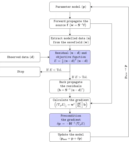
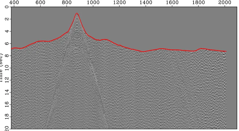
1.1 A basic workflow for a single iteration in conventional FWI. If it is the first it-eration, the parameter modelp is the initial model obtained by other techniques, for example first arrival traveltime tomography. The blue coloured boxes indicate those steps in the workflow to which this study contributes. Upper caseT in the superscript represents matrix transpose and complex conjugation, lower caset rep-resents only transpose, and⇤represents complex conjugation only. . . 6 1.2 An example receiver gather from ocean bottom sensor (OBS) 74 from the ocean

bottom wide-angle velocity experiment (OBWAVE) survey. The vertical axis is reduced time, and the horizontal axis represents the sources located 8 m below the surface of the ocean. Receivers were placed on the ocean bottom, which had a depth of 1.9 km. The reduction velocity in this figure is 8 km/s. The red line

represents the first break pick, which mark the arrival of the earliest signal on the receiver. Due to the reciprocity of the Green’s function, this can also be viewed as a source/shot gather. . . 7

1.3 Sensitivity kernels with a constant background velocity: Source is at (x,z) =

(0.6,0) km, receiver is at (x,z) = (1.4,0) km and there is a sharp horizontal

re-flector (a continuous distribution of scatterers along a line) at 0.8 km depth. There are three sensitivity kernels: to-reflector, reflector-to-receiver and source-to-receiver. The source-to-receiver sensitivity kernel is due to the direct arrivals (top part), that is first order scattering. The source-to-reflector and reflector-to-receiver sensitivity kernels are due to second order scattering. . . 10

2.1 Model scales (after Wu and Toksöz, 1987). Between kb andkmax the background

(11)

wavenumber information will be included before the background velocity model has converged, therefore it can potentially move the inversion away from the true solution. . . 27 2.3 (a) A test image, and (b) its wavenumber amplitude spectrum. . . 38 2.4 (a) The SSP applied to the test image (Figure 2.3), with⇣µ2₀, µ2₁⌘ =(1,100), and (b)

its wavenumber amplitude spectrum. . . 39 2.5 (a) Gaussian smoothing applied to the test image (Figure 2.3) with 2 ₌ _100,

and (b) its wavenumber amplitude spectrum. The small non-zero amplitude re-gion around the origin in (b) shows the almost complete loss of high wavenumber information after Gaussian smoothing. . . 39 2.6 Gaussian smoothing applied to the test image (Figure 2.3), with (a) 2 ₌ _{50, (b)}

2 ₌ _{10, (c)} 2 ₌ _{1 and (d)} 2 ₌ ₀_._{5. Decreasing the scale factor of the Gaussian}

smoothing reduces the weights of the low-wavenumber features, however the high wavenumbers in the image are lost. To preserve the edges, the scale factor has to approach zero, in which case the low-wavenumber features are no longer enhanced. 40 2.7 Direct comparison of the smoothing kernels: (a) Sobolev pre-conditioning with

⇣

µ2₀, µ2₁⌘ = (1,0.1), (b) Gaussian smoothing with 2 = 0.1,and (c) Gaussian

smoothing with 2 ₌ ₀_.₀₃₅_. _{(d) Profiles extracted from (a) to (c) at zero}

verti-cal wavenumber, where the blue line is from (a), the green line is from (b), and the red line is from (c). Decreasing the Gaussian smoothing in an attempt to en-hance the high-wavenumbers broadens the Gaussian bell-shaped curve (note the shift from the green to red lines), but the higher wavenumber are still not recovered to the level of SSP (blue line). . . 42 2.8 (a) The true velocity model used in the inversion tests, and (b) the linear 1D starting

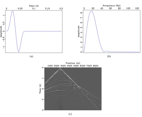
velocity model. Vertical lines in the figures represent the locations where velocity profiles will be compared. . . 43 2.9 (a) The Küpper source wavelet used in the inversion tests, (b) its amplitude

spec-trum, and (c) a representative synthetic observed shot gather atx= 2536 m. . . 44

2.10 Representative ray paths in the true (Marmousi) model with sources located at: (a) 2 km, (b) 4 km, (c) 6 km and (d) 8 km. The recievers are located along the horizontal white line atz=160 m. . . 45

2.11 An image of the objective function gradient (a) before and (b) after SSP (pre-conditioning) with⇣µ2₀, µ2₁⌘ = (1,50), at the 173rd iteration in the SSP inversion.

(12)

2.12 The objective function gradients in the inversion with Gaussian pre-conditioning, (a) before and (b) after Gaussian smoothing with 2 ₌ _{50, shown at the 173}rd

iteration. No o↵set-dependent exponential gain was applied to the data in this test. 47

2.13 Final inversion results without o↵set-dependent exponential gain after 650

itera-tions, for (a) the SSP inversion and (b) for Gaussian pre-conditioning. In the final stages minimum values of the SSP scalars ⇣µ2₀, µ2₁⌘ = (1,10), and the Gaussian

smoothing scalar 2 ₌₀_._{were used. . . 48}

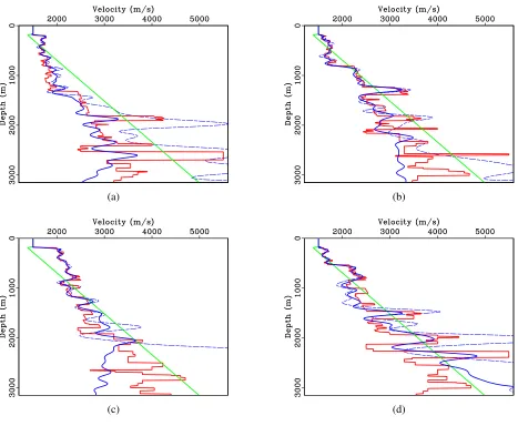
2.14 Velocity profiles from the final inversion results in Figure 2.13, at (a) 2 km, (b) 4 km, (c) 6 km and (d) 8 km: The red line depicts the true velocity model and the green line depicts the starting velocity model. Solid and dashed blue lines are SSP and Gaussian pre-conditioning results, respectively. . . 49 2.15 Comparison of squared residuals vs iteration history for the SSP mthod and for

the Gaussian method, for inversions without o↵set-dependent exponential gain,

showing (a) all iterations from 1 to 650, (b) iterations 1-20, (c) iterations 20-200, and (d) iterations 200-650. . . 50 2.16 An image of the objective function gradients (a) before, and (b) after SSP

(pre-conditioning) with⇣µ2₀, µ2₁⌘ = (1,10), at the 217th iteration in the SSP inversion.

O↵set-dependent exponential gain was applied during this test. . . 51

2.17 The objective function gradients in the inversion with Gaussian pre-conditioning (a) before, and (b) after Gaussian smoothing with 2 ₌ ₁₀_, _{shown at the 11}th

iteration. . . 52 2.18 Final inversion results without o↵set-dependent exponential gain, after 365

iter-ations (a) for SSP and (b) for Gaussian pre-conditioning inversions. In the final stages minimum values of the SSP scalars ⇣µ2₀, µ2₁⌘ = (1,0.1), and the Gaussian

smoothing scalar 2 ₌₀_._{1 were used. . . 52}

2.19 Velocity profiles in Figure 2.18 at (a) 2 km, (b) 4 km, (c) 6 km and (d) 8 km: The red line depicts the true velocity model and the green line depicts the starting velocity. Solid and dashed blue lines are the SSP and Gaussian pre-conditioning results, respectively. . . 53 2.20 Comparison of squared residuals vs iteration history for the SSP method (solid

curves) and for the Gaussian method (dashed curves), for inversions with o↵

(13)

between the red and the green functions in both (a) and (b) will be small because the function values are close to each other. A derivative based inner product of the di↵erence between red and blue functions will be large for (a). For (b), a derivative

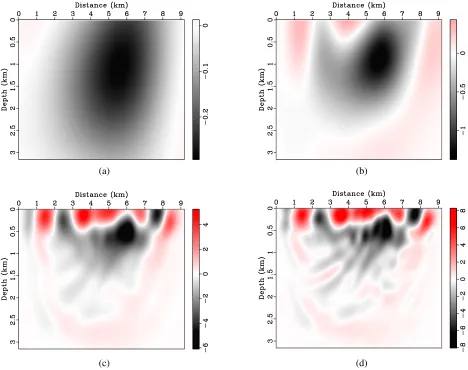
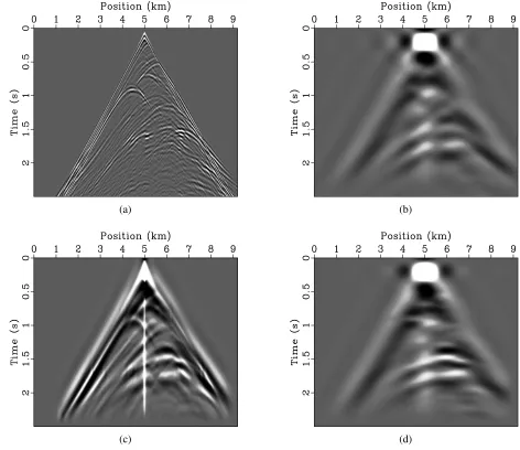
based inner product can be small if the red and blue curves are shifted relative to each other. . . 67 3.2 Comparison of frequency-wavenumber filtering with data domain SSP.!andkrare

the circular frequency and receiver wavenumber, respectively. Unfiltered data are shown in (a) and pre-conditioned data with SSPM= 5 andµ2₀= 0.1 in (b). The

fre-quency filtered data (!_ 2.5 Hz)are shown in (c), and frequency and wavenumber

filtered⇣!,kr 2.5 Hz,0.75 km 1⌘data in (d). For SSP in (b)⇣µ2₉, µ2₁₀⌘= (0.077,1.0). 72

3.3 SSP parameter e↵ects: (a), (b) and (c) were computed with⇣µ2₅, µ₆2⌘ = (0.077,1.0)

and (d) with⇣µ2₉, µ2₁₀⌘= (0.077,1.0). The maximum SSO orderMandµ0values are ⇣

M, µ2₀⌘ =(3,1), (3,0.01), (3,0.1) and (5,0.1) for (a), (b), (c) and (d) respectively. 73

3.4 Real part of the complex data residuals for 8 Hz. (a) Before and (b) after SSO pre-conditioning. In both figures the units are arbitrary. Red color represents positive value, blue represents negative value and green is zero. . . 78 3.5 SSO pre-conditioning along source and receiver axes only. Gradients at iteration 2

without (a) and with (b) model domain SSP. . . 79 3.6 Marmousi (a) and starting velocity (b) models. The starting velocity has been

smoothed and bulk reduced by 30%. Vertical lines are the locations of velocity profiles. . . 79 3.7 (a) The Küpper source wavelet used in the inversion tests, (b) its frequency

spec-trum. . . 80 3.8 Sensitivity kernes for 8 Hz. (a) O↵set 5760 m and (b) 7776 m. Both sensitivity

kernels were generated with a time domain damping factor of 1 s. . . 81 3.9 Inverted model after 280 iterations (a) with and (b) without temporal scale

pertur-bation. The inversion with temporal scale perturbation manage to bring in more sharper features than in the one without temporal scale perturbation, in the same number of iterations. . . 83 3.10 Vertical velocity profiles at (a) 2000m, (b) 4000 m, (c) 6000 m and (d) 8000 m,

(14)

3.11 Inverted model with SSO and temporal scale perturbation. As indicated by the shaded region, the inversion is reliable only down to a depth of about 1500 m. This was because of the shallow sensitivity kernels . . . 85

4.1 Map of the OBWAVE survey (after Watremez et al., 2015). The red line shows the source positions (i.e., the trajectory of the ship) and the black dots are OBS locations. 97 4.2 The 2D OBWAVE survey geometry with (a) all sources and receivers and (b) only

those sources and receivers that were used in FWI. The green dot in (a) is an OBS location that was not used in FWI. OBS locations are shown with cyan and red dots for eastern and western lines, respectively. Using the same colour coding, the lines on the surface represent sources (the sources are actually points that are approximately 140 m apart, so they appear to be a continuous line in the figure). The background of the figures shows the first 7 kms of the first arrival traveltime inversion by Watremez et al., 2015. . . 100 4.3 Amplitude spectra of OBS 35. Red is the raw data and blue is the pre-processed

data. The green lines represent the extent of the bandpass filter applied in data pre-processing. . . 101 4.4 Pre-processed data for (a) OBS 35 (b) OBS 74, plotted in reduced time with a

reduction velocity of 8 km/s. The red line shows the first break picks. . . 102

4.5 Stacking chart and the traveltime tomographic model used as the initial velocity in FWI. The presence first break picks used in traveltime inversion by Watremez et al. (2015) is indicated by green and black lines for each OBS, and the red lines in the OBS profiles indicate an absence of first break picks. The black line of the OBS profile indicates that the data were not used in the FWI (despite the presence of first break picks) because they were outside of the model region being inverted. The western line is between the two vertical red lines and the eastern line is on the left of the second red line at 296 km. . . 103 4.6 The traveltime tomographic model used as the initial velocity in FWI for (a) eastern

and (b) western lines. . . 104 4.7 Sensitivity kernels between OBS 45 and 84 (West) at (a) 2 Hz (b) 8 Hz using

traveltime tomographic model. Using the same model, sensitivity kernels were also calculated between OBS 18 and 36 (East) at (c) 2 Hz and (d) 8 Hz. . . 105 4.8 Modelled data using the initial velocity model for (a) OBS 35 (b) OBS 74 plotted

(15)

of a surface seismic experiment for a given frequency. Anisotropic SSP filters indicated by blue contours and the isotropic SSP by red contours. . . 109 4.10 (a) Raw, (b) pre-conditioned and (c) conjugate gradient at 79th _{iteration from the}

western line. . . 111 4.11 Initial source inversions in the eastern line (a) for all OBSs and (b) their average.

Initial source inversion in the western line (c) for all OBS and (d) their average. . . 117 4.12 Raw gradients at the end of (a) stage 1, (b) stage 2, (c) stage 3 and (d) stage 4 from

the western line. The ends of stages 1, 2, 3 and 4 were at iterations 50, 70, 90 and 120, respectively. . . 119 4.13 SSP gradients at the end of (a) stage 1, (b) stage 2, (c) stage 3 and (d) stage 4 from

the western line. The ends of stages 1, 2, 3 and 4 were at iterations 50, 70, 90 and 120, respectively. . . 120 4.14 Velocity di↵erence east: Initial velocity subtracted from the inverted velocity at the

end of (a) stage 1, (b) stage 2, (c) stage 3 and (d) stage 4 from the eastern line. The ends of stages 1, 2, 3 and 4 were at iterations 50, 70, 105 and 135, respectively. . . 121 4.15 Velocity di↵erence west: Initial velocity subtracted from the inverted velocity at

the end of (a) stage 1, (b) stage 2, (c) stage 3 and (d) stage 4 from the western line. The ends of stages 1, 2, 3 and 4 were at iterations 50, 70, 90 and 120, respectively. . 122 4.16 Final inverted velocity model for the eastern line (a) and its di↵erence with the

initial velocity (b). Final inverted velocity model for the western line (c) and its di↵erence with the initial velocity (d). . . 124

4.17 Eastern line source inversions for quality control using a cosine o↵set taper to

re-move near o↵sets. The taper started at 10 km and ended at 15 km. Source inversion

with initial velocity (a) for all OBSs and (b) their average. Source inversion with final velocity (c) for all OBSs and (d) their average. . . 125 4.18 Western line source inversions for quality control using a cosine o↵set taper to

re-move near o↵sets. The taper started at 10 km and ended at 15 km. Source inversion

with initial velocity (a) for all OBSs and (b) their average. Source inversion with final velocity (c) for all OBSs and (d) their average. . . 126 4.19 Modelled data using the final velocity model for (a) OBS 35 (b) OBS 74, plotted

in reduced time with a reduction velocity of 8 km/s. . . 127

(16)

Chapter 1 Introduction

Seismic full waveform inversion (FWI) aims to recover a set of subsurface parameter models that best explain the observed seismic data. This task is complicated by the fact that FWI is an in-herently non-linear problem (Tarantola, 1984). FWI can be linearized under certain assumptions. However, these assumptions do not always hold, and considerable e↵ort is required to mitigate the

non-linearity. Before getting into the details, let us put things into perspective by having a quick look at the evolution of the seismic method and some of the major contributions that brought the ambitious goal of FWI within our reach.

1.1 Evolution of the seismic method

The first controlled source seismic experiment was conducted (Mallet, 1846, 1851) to measure the speed of the tremors generated by the source. These early measurements were inaccurate mainly due to the insensitivity of the seismometer used. However, this marks the beginning of the seismic method, in that the idea to measure the first arrival times of the tremors generated from a controlled source as a means of calculating the velocity is still indispensable in the seismic method to this day. Throughout the latter half of the century, those measurements were improved and considerable theoretical advancements were made towards understanding the physics of wave propagation in the earth. By the early twentieth century, scientists had already developed the theoretical and experimental framework necessary to explore the subsurface, and started to realize the economic potential of the seismic method (Weatherby, 1940).

(17)

applied in 1919, Mintrop, 1926). This process is still used in seismic data processing However it has some inherent limitations, which were soon realized. First of all, the subsurface layers have to be increasing in velocity, and the sharper the contrast in velocity, the better identification of the layers in the data. This limitation resulted in some failures of the refraction profiling method when applied in California (Weatherby, 1940), where there were no intrusive salt domes to give a high velocity contrast. As the refracted arrivals from deeper layers require far o↵sets to be recorded,

the source had to be powerful in order to enhance the first arrivals at those o↵sets; given the low

sensitivity of the seismometers at that time. Therefore, refraction profiling was a costly operation, especially if deeper formations had to be studied. Another issue was the lack of resolution as a result of using only the first arrival times. This might sound familiar to a modern day waveform tomographer.

1.1.1 Imaging with reflections

The problems with refraction profiling were not shared by another method that used reflections instead of refractions from the subsurface formations (Weatherby, 1940; Dragoset, 2005). The use of seismic reflections in locating geological formations was first proposed by Reginald Fes-senden (Patent applied for in 1914, FesFes-senden, 1917). The first seismic reflection experiment was carried out by a team including John C. Karcher in 1921 (Karcher, 1987), using his newly devel-oped equipment for the seismic reflection method. The experiment was performed near the Vines Branch area in south-central Oklahoma. The seismic reflection method constructs an image of the subsurface formations by estimating the depth of the reflector using the two-way traveltime of the reflected events in the data, assuming the velocity is known. Based on a constant velocity, the possible reflection points for an event in the data (in two dimensions, 2D) are constrained to be on a circle in the vertical plane parallel to the source/receiver lines. If such a circle is drawn for all

events, the continuous curve that is tangent to these circles gives the seismic image with true re-flector position. This was the method used to construct the image in the Vines Branch experiment. Although not named as such, the image construction method used in the Vines Branch experiment was also the first application of what is now called seismic migration. During the three decades after the Vines Branch experiment, improvements were made in the reflection profile by increasing the seismometers/geophones per shot and understanding of the e↵ects of complex geology (faults

and folds) on reflections (Bednar, 2005).

Major advances were made in the 1950s and 1960s. Hagedoorn (1954) proposed a migration process that is now known as the Kirchho↵summation; Dix (1955) presented a method to calculate

(18)

CHAPTER 1. INTRODUCTION

computing of the seismic data allowed the full potential of these methods to be utilized (Dragoset, 2005). By using the moveout equation on CMP sorted data, it became possible to determine the velocity of the subsurface formations.

With advances in computational capacity, that is the introduction of digital computers in the 1960s, it was possible to apply velocity determination (velocity analysis) and migration much more efficiently (Dragoset, 2005). This paved the way for wave equation based migration techniques

that were able to handle lateral velocity variations to varying degrees. Claerbout (1971) suggested a method that made use of a one way wave equation, and Stolt (1978) suggested a frequency-wavenumber domain migration, which was valid with only a constant velocity. With the use of a one-way propagator the migration could handle vertical velocity variations However, it was limited in the dips that it could handle and did not take the true amplitudes into account (Bednar, 2005). In an integral formulation, Kirchho↵migration (equivalent to di↵raction stack) was able to handle

all dips as long as there was enough aperture and the kinematic part of the Green’s function could be calculated (Schneider, 1978). The surest way possible (as long as the linear theory of elasticity is applicable) to take all amplitude and multiple scattering into account is to image with the full two-way wave equation. Baysal et al. (1983) proposed using the two-way solution to the wave equation, which is the imaging technique known as reverse time migration (RTM).

There has been a substantial amount of work done towards solving some of the outstanding problems of seismic imaging, for example multiple attenuation/imaging (Verschuur et al., 1992;

Bakulin & Calvert, 2006) and multi-component processing (Sava & Alkhalifah, 2012). However, in order to pursue a more general solution than what seismic imaging can o↵er, we would have to

part ways with imaging at this point and move towards the more ambitious task of seismic inversion and the non-linearity therein.

1.2 Seismic Inversion

If seismic imaging is treated as an inverse problem, that is to find a velocity model that can repro-duce the observed data, we can potentially find the true subsurface velocity. This reformulation of imaging was proposed by Lailly (1983); Tarantola (1984) and Tarantola (1984), where the objec-tive of the inversion was to minimize theL2_{-norm of the di}_↵_{erence between observed and simulated}

seismic data. The most important contribution of these studies was the realization that the gradient of such an inversion scheme can be obtained by a pre-stack migration, that is migrating the data residual before stacking1_{the data. This was important because otherwise each spatial point in the}

model would have to be perturbed independently and with it a forward modelling step performed, thus rendering the method computationally infeasible (Tarantola, 1984). Although the inverse

(19)

method had the promise of giving true scatterer amplitudes, it was still reliant on the fact that the background velocity model is required, just like conventional seismic imaging. The least squares objective function depends non-linearly on the background velocity and linearly on the scatterers, as noted by various authors (Jannane et al., 1989; Symes, 1991). It had already been recognized that in order to make the solution of the inverse problem more general than just a true amplitude pre-stack depth migration, the background velocity had to be recovered in order to successfully invert for the scatterers (Snieder et al., 1989; Cao et al., 1990). A definite proof of the fact that the transmitted part of seismic data contains the information required to update both background and scatterers was given by Mora (1987, 1988) and Pratt & Worthington (1990); Pratt (1990a), where the former used the wave equation in the time domain and the latter did the same in the frequency domain for forward modelling. These studies also highlighted the importance of using long o↵

-set data to obtain low wavenumbers in the inverted model, as explained by Wu & Toksöz (1987), thereby updating the background (by using long o↵sets) and reflections/di↵ractions together. This

was a giant step towards a complete solution that gives the subsurface parameters for all spatial scales scales, that is full waveform inversion. In a sense, we have come a full circle from Ludger Mintrop’s refraction profiling method, in that the refracted arrivals and far o↵sets have again taken

the centre stage in exploration seismology.

1.3 Non-linearity in full waveform inversion

Combining the background and scatterer inversions makes the FWI a more comprehensive tech-nique, however the problem is not completely solved. Even with the full wave equation as a forward propagator, the FWI problem is usually linearized using the Born approximation2 _(Pratt

et al., 1998). This, along with the fact that seismic data contain a finite bandwidth, implies that a background velocity that gives traveltime errors greater than half-cycle would lead to a false min-imum (Beydoun & Tarantola, 1988; Pratt, 2008; Virieux & Operto, 2009). This non-linearity is the essential problem in FWI. This form of non-linearity is known as cycle-skipping, and it serves as a criterion for the background velocity for which FWI is linear known as “the half-cycle crite-rion”. Pratt (2008) reformulated this as a relation between the relative traveltime error⇣ t

T ⌘

and the number of wavelengths (N ) contained in the total path length of the wave, that is

t T <

1

2N . (1.1)

The dependence on the number of wavelengths means that far o↵sets are more prone to cause

2_{Physically, the Born approximation means assuming that the wave scattered only once. This is mathematically}

(20)

non-linearity in FWI by cycle-skipping.

1.3.1 Initial model

Naturally, the surest possible way to avoid cycle-skipping in FWI is to have the arrivals in the starting model satisfy the half-cycle criterion. First arrival traveltime tomography (Nolet, 1987b; Woodward, 1992) is one such approach, where the first arrival times from the data are inverted to produce low wavenumber velocity model. The resolution limit of first arrival traveltime to-mography is is determined by the width of the first Fresnel zone (Williamson, 1991). This gives much lower resolution than FWI, which is of the order of the wavelength at the scatterer (Huang & Schuster, 2014). The first arrival traveltime inversions cannot guarantee that events other than the first arrivals will be explained (Virieux & Operto, 2009). This is because a small error in the low wavenumber component in the model might cause cycle-skipping for sufficiently late arrivals

in the data. Since first arrival traveltime tomography is itself an inherently non-linear problem (Nolet, 1987b; Woodward, 1992; Zelt & Barton, 1998), such errors in the inversion would not be unexpected, especially when the first break pick are not reliable (for example due to noise in the data). Nonetheless, if the seismic data contain far o↵sets and low frequencies, these problems can

be overcome (Pratt & Goulty, 1991; Ravaut et al., 2004; Brenders & Pratt, 2007b,a).

First arrival traveltime tomography can also be modified to include reflections in the inversion process. For example, Watremez et al. (2015) used a method suggested by Korenaga et al. (2000) for inverting both refraction and reflection traveltimes on the OBWAVE acquired in o↵shore

New-foundland to delineate the Moho boundary.

1.3.2 A typical FWI workflow

A typical workflow of FWI for a single iteration is shown in Figure 1.1. The starting parameter modelpis used to forward propagate a source functionf. Using matrix-vector notation, the wave equation in Frequency domain can be written asSw= f, wherewandSare the wavefield and the

di↵erencing matrix, respectively. Each element inwrepresents the wavefield at a point in space.

The modelled datauare extracted from the wavefieldwat the receiver locations. An example of surface seismic data is shown in Figure 1.2. The receiver gather in Figure 1.2 is plotted in reduced time3_{, which allows inverting for later arrivals without using the whole record length. The observed}

datadare then subtracted fromuand the objective functionEis calculated. The objective function used in conventional FWI is the sum of squared residuals

3_{Time reduction means subtracting a time given by a linear function of source-receiver o}_↵_{set from the recording}

timetof each trace i.e.⇣treduced=t _{reduction velocity}(xsou xrec)

⌘

, wherexsouandxrecare the lateral positions of source and receiver,

(21)

Parameter model (p)

Forward propagate the

sourcef w=S 1_f

Extract modelled data(u)

from the wavefield (w)

Residual(u d) and

objective function

E = 1₂(u d)T (u d)

Observed data(d)

Back propagate the residuals

b=S 1₍_u _d₎⇤

Stop

If E >Tol.

Calculate the gradient_⇣

(rpE)_j =wt h

@St @pj

i

b⌘

Precondition the gradient

p = H 1(_rpE)

Update the model

(pnew=p+ p)

pnew

!

p

IfE <Tol.

2

(22)

Figure 1.2: An example receiver gather from ocean bottom sensor (OBS) 74 from the ocean bottom wide-angle velocity experiment (OBWAVE) survey. The vertical axis is reduced time, and the horizontal axis represents the sources located 8 m below the surface of the ocean. Receivers were placed on the ocean bottom, which had a depth of 1.9 km. The reduction velocity in this figure is 8 km/s. The red line represents

(23)

E = 1

2(u d)T(u d), (1.2)

where T _{represents transpose and complex conjugation, and the di}_↵_erences _{u d} _{are known as}

the data residuals. However, there can be other choices, for example Shin & Min (2006) proposed using the logarithm of the ratio of modelled and observed data known as the “logarithmic residual”. Kamei et al. (2014) discussed some possibilities for objective functions, for example the phase-only inversion. In a phase-only inversion the di↵erence is calculated between modelled and observed

data after the amplitudes have been set equal to one in both datasets. Kamei et al. (2014) also suggested a phase-only version of the logarithmic residual. This step of the FWI process is one of the places where this study modifies the conventional workflow by introducing a new objective function. Once the objective function is calculated its value is tested against a predefined tolerance. IfE <Tol. the inversion is stopped, and the model at the start of the current iteration, sayp, is the

result of the inversion, otherwise the inversion continues. IfE >Tol. then in conventional FWI, the residual is back propagated. In general, for any objective function the quantity used to obtain the back propagated field is called the adjoint source, which is determined by the adjoint state method (Plessix, 2006). The back propagation then gives the back propagated wavefieldb. Thenbandw

are multiplied in the frequency domain to give the conventional FWI gradient. After Pratt et al. (1998), the jth_{component of the gradient is given as}

⇣ rpE

⌘ j = w

t"@St

@pj #

b, (1.3)

wheret means transpose without complex conjugation and the partial derivative of S consists of a non-zero value only at the jth _{model point. The gradient can then be pre-conditioned with an}

operator. For Newton method, the pre-conditionerH 1 _{is the inverse Hessian. If it is the inverse}

of some approximation of the Hessian, the inversion is called Gauss-Newton or quasi-Newton method, depending on the type of approximation. In the steepest descent methodH 1_{is replaced}

by an identity matrix scaled by a real positive scalar, which is called the step length. For pre-conditioned steepest descent a positive definite pre-conditioner is also multiplied by the gradient. This is one of steps modified in this study, where an edge preserving pre-conditioner will be used for model scale separation. The negative of the pre-conditioned gradient is the model perturbation. The starting model for current iterationpis updated by adding the model perturbation to obtain a new parameter model, saypnew. Finally,pis set equal topnewand another iteration starts.

1.3.3 Scale separation

(24)

wavenumber updates. This also suggests that the background should be updated before the scatter-ers (sharper features of the model) are taken into account (Snieder et al., 1989; Cao et al., 1990), which is the essence of the multiscale approach. Either in the time domain (Bunks et al., 1995) or in the frequency domain (Pratt & Worthington, 1990), the basic idea is to separate the temporal scales of the data by starting FWI with the lowest available frequency (large temporal scale) and bringing in higher frequencies (small temporal scale) at later iterations. Separating the scales in the time domain naturally implies a spatial scale separation in the gradient, in that low frequency inversion results in low wavenumber gradients.

Using a multiscale approach along with using far o↵sets in the data adds a second tool by

which the model scales may be separated in order to update the background and thereby mitigate the non-linearity in FWI (Brenders & Pratt, 2007b). Low wavenumbers in the gradient can also be enhanced by damping later arrivals in the data in time domain. This would enhance early arrivals, which are dominated by refracted events, thereby constraining N and mitigating non-linearity in FWI (Kamei et al., 2013). As the data amplitudes are often dominated by near o↵sets,

low wavenumbers in the gradient can be enhanced by weighting the far o↵sets using an o↵set

dependent gain.

Using far o↵sets to enhance low wavenumber in the gradient implicitly assumes single

scatter-ing with a large angle (Wu & Toksöz, 1987). This can be seen with an argument followscatter-ing Virieux & Operto (2009), who in turn refer to Pratt & Worthington (1990) and Wu & Toksöz (1987). The relationship between the scattering wavenumber (k), frequency (f) and di↵raction/scattering angle

(✓) is

k= 2f

c cos

✓_✓

2

◆

n, (1.4)

where c is a constant velocity and n is a unit vector in the direction of the sum of incident and negative of the scattered directions. It can be seen from equation (1.4) that a small scattering angle would lead to a small scattering wavenumber, which represents the wavenumber content of the gradient in FWI (Wu & Toksöz, 1987). Since the scattering angle (✓) is related to the

source-receiver o↵set, the scattering wavenumber (k) in equation (1.4) can be controlled by varying

either frequency or o↵set, thereby resulting in a redundancy in scattering wavenumber information.

Sirgue & Pratt (2004a) use this redundancy to select larger frequency intervals where far o↵sets are

(25)

Reflector

Figure 1.3: Sensitivity kernels with a constant background velocity: Source is at (x,z)=(0.6,0) km, receiver is at (x,z)=(1.4,0) km and there is a sharp horizontal reflector (a continuous distribution of scatterers along

a line) at 0.8 km depth. There are three sensitivity kernels: source-to-reflector, reflector-to-receiver and source-to-receiver. The source-to-receiver sensitivity kernel is due to the direct arrivals (top part), that is first order scattering. The source-to-reflector and reflector-to-receiver sensitivity kernels are due to second order scattering.

background update. The main advantage of using rabbit-ears to obtain low wavenumber updates is that it does not require long o↵sets. This fact is used in the joint full waveform inversion (JFWI)

proposed by Zhou et al. (2015). In JFWI reflections are imaged by using smaller o↵sets and the

diving waves are taken into account by using far o↵sets However, reflection updates can su↵er

from cycle-skipping unless a-priori information about the reflectivity is used.

Guitton et al. (2012) showed that using a pre-conditioning of the gradient that is constrained by local dip information in the gradient (possibly through the technique proposed by Hale (2007)) can help with convergence for low-wavenumber updates. Guitton et al. (2012) also show that edge-preserving smoothing can help in reducing the acquisition footprint of an irregular geometry and in reducing artifacts due to the presence of coherent noise. This approach is di↵erent from the

others discussed so far, in that edge-preservation smooths the gradient while preserving the sharper features. Therefore, the method proposed by Guitton et al. (2012) is an example of constrained scale separation in the model domain. Edge-preserving smoothing has also been used in the field of image processing, where methods such as anisotropic di↵usion (Perona & Malik, 1990),

(26)

1.3.3.1 Sobolev space

Generally, edge-preservation can be achieved by considering the derivatives of the image in the smoothing process. For example, TV methods for denoising minimize the energy of the spatial derivatives of the image. The energy of a continuous-time signal f(t) is defined R1₁|f (t)|2dt, mathematically this is the square of an L2_{-norm of a function} _f₍_t_{). This suggests that when the}

energy of a derivative of a signal is considered, it would be convenient to work in a space of functions that has a norm that takes the derivatives of a function into account. Sobolev space is such a space and it would not be out of place to say a few words about the Sobolev space.

The Sobolev space was originally introduced to study the solutions of partial di↵erential

equa-tions (Evans, 2010). For our purpose in this study it would be more useful to look at an intuitive picture. The three physical dimensions of space form a set of points in space. Each point can then be assigned a “position vector” and that set of vectors becomes a “vector space” if all vectors satisfy certain conditions4_{. There has to be a “structure” added to this vector space for it to be}

useful in physical applications. This structure is the notion of a distance between two points or vectors. For two vectorsu andv, this distance is the square root of the inner/dot product, that is

d (u,v) _{⌘ k}u v_{k ⌘} p(u v)_·(u v)= qP3_i₌₁(ui vi)2. Note that the distance function is

non-negative, in fact this is the only requirement that the distance function has to satisfy, the existence of an inner product is optional. Mathematically the distance function is known as the “norm” (that measures the length of a given vector) of this space, which is the familiar “Euclidean space”. With a norm defined, consider a series of vectors with decreasing lengths such that the sum of the vector lengths in the series is finite. Then if we demand that the sum of all vectors in that series is again a vector in the Euclidean space, the Euclidean space is said to be complete.

If instead of vectors we consider a set of functions that satisfy the properties above we get a function space, known as the Hilbert space. More formally, a Hilbert space is a complete vector space with a norm defined as the square root of an inner product. If only the distance function is defined without relying on an inner product, we have a Banach space or formally a complete vector space with a norm. Now let us consider a Banach space with a norm that includes derivatives of a function and denote this byWk,p₍_⌦_{), where}_k_{is the maximum order of derivatives in the norm,} _p

is the exponent and⌦ represents the domain of the functions in the space. The spaceWk,p(⌦) is

known as the Sobolev space. For functions of a single real valued variable the Sobolev space can be denoted asWk,p₍_R₎_._{with the norm given as}

kf_kWk,p ⌘

0 BBBBB @

k X

i=0 Z

f(i) p_d_t 1 CCCCC A 1 p = Z

|f_|p_d_t₊_{· · ·}₊Z @kf

@k_t p

dt

!1 p

. (1.5)

4_{Associativity and commutativity of addition, existence of identity and inverse of addition, and compatibility and}

(27)

With p = 2 in equation (1.5) the Sobolev space Wk,2(⌦) becomes a Hilbert space denoted as

Hk₍_⌦_{). If the functions are further assumed to vanish at the domain boundary, the Hilbert space}

Hk₍_⌦_{) is denoted by}_Hk

0(⌦). The inner product and norm forHk0(R) can be written as

hf, f_iHk 0 ⌘

k X

i=0 Z

f(i) 2_d_t =

Z

|f_|2_d_t

+· · ·+

Z _@k_f

@kt

2

dt (1.6)

and

kf_kHk 0 ⌘ 0 BBBBB @ k X

i=0 Z

f(i) 2_d_t 1 CCCCC A 1 2 = 0 BBBBB @ Z

|f_|2_d_t₊_{· · ·}₊Z @kf

@k_t 2 dt 1 CCCCC A 1 2 , (1.7) respectively.

In this study we will be interested in the Sobolev space Hk

0(⌦), which is also a Hilbert space.

The Hk

0(⌦) is of interest because it consists of functions that are smooth or “regular”. The

re-quirement of smoothness is implied by the rere-quirement that the functions are di↵erentiable up to

a certain order. Another desirable property is that the distance between two function will depend not only on the values of the functions but also the values of their derivatives. This can be seen from equation (1.7) if f is replaced by g h, whereg,h✏ H₀k(⌦). However, as they stand

equa-tions (1.6) and (1.7) do not lend themselves easily for use in separation of scales. This is because each derivative order in the inner product cannot be weighted independently. This issue of scaling di↵erent derivative orders will be addressed in this study by defining an inner product that gives a

scaled version of the Sobolev⇣Hk 0(⌦)

⌘

norm, that is the scaled-Sobolev inner product.

1.3.3.2 Data domain

As described above, model scale separation can be achieved by pre-conditioning the observed data. We have already seen some examples, like time domain damping and o↵set weighting. The

conventional L2_{-norm objective function can also be modified for example by including the data}

and model covariance matrices, allowing a priori information about the data or model to be taken into account (Tarantola, 1984). Tikhonov regularization can also be used to smooth the gradients (Asnaashari et al., 2013), where anL2_{-norm of the spatial derivatives is added to the conventional}

data misfit function. This acts as a constraint that penalizes any roughness in the model updates. However, smoothing alone would remove high wavenumber features completely. Asnaashari et al. (2013) add both a first-order Tikhonov term and an a priori information term to the conventional misfit. If the a priori information contains high wavenumber features, the total objective function can act as a constrained scale separation as in Guitton et al. (2012).

The conventionalL2_{-norm objective function can also be replaced by a Sobolev norm that takes}

(28)

propose a di↵erential semblance approach5that di↵erentiates the residuals along the receiver axis.

The rate of change data with respect to o↵set is highest for large angle scattering (where the phase

of the data changes rapidly, Snieder (2004)), therefore in this approach far o↵sets will be enhanced.

Therefore, this approach would enhance low wavenumbers in the model due to the wide angle nature of large o↵set data.

1.4 Frequency domain modelling and source estimation

Forward modelling in FWI can be performed in either the time domain (Tarantola, 1984; Gauthier et al., 1986; Mora, 1987) or in the frequency domain (Pratt, 1990b; Pratt & Worthington, 1990). In this study only frequency domain approach is used (with acoustic approximation) , after Pratt (1990b). In the frequency domain, the computational cost can be reduced by inverting fewer fre-quencies However an inversion of the di↵erencing matrix6 is demanding in terms of memory, as

discussed by Pratt (1990b) frequency domain finite di↵erence implementation. Although this

lim-itation can be mitigated by using techniques like nested dissection (Pratt, 1990b; George & Liu, 1981), the matrix inversion inversion would become impractical for 3D modelling. Nonetheless, 2D inversions are useful to study some of the theoretical and practical aspects of FWI. Another advantage of the frequency domain modelling is that attenuation can be taken into account rather easily, that is by making the velocities complex (Kamei et al., 2013). Moreover, a data domain pre-conditioning can also be applied by using complex rather than real frequencies (Sirgue & Pratt, 2004a; Brenders & Pratt, 2007b; Shin & Cha, 2009), that is Laplace-Fourier domain method. Brenders & Pratt (2007b) show that the Fourier transform of an exponentially damped function in time domain is equivalent to a Laplace transform. Therefore, by choosing an appropriate damping factor as the complex part of the frequency, a time domain damping can be applied to the data. This is useful in pre-conditioning the data to obtain very low wavenumber velocity models that also can serve as a starting model in FWI (Shin & Cha, 2009; Virieux & Operto, 2009). Since the di↵

erenc-ing matrix is independent of the source function, once it has been factorized it can be stored and used for all sources, which means that the computation cost does not increase significantly with the number of sources (Pratt, 1990b). The di↵erencing matrix has to be inverted/factorized for

every frequency However, each frequency component of the wavefield is independent. Therefore, the Laplace-Fourier domain modelling can be parallelized over frequencies (Kamei et al., 2013).

5_{The term di}_↵_{erential semblance refers to measuring the similarity of a function, whether seismic data or image,}

along source receiver o↵set axis. The similarity measure is the magnitude of the derivative of the function along the o↵set axis.

6_{The di}_↵_{erencing matrix is a sum the discrete representation of the Laplacian and a diagonal matrix of frequency}

term in the wave equation. For the acoustic wave equation⇣r2₊!2

v2 ⌘

u= f can be written in matrix-vector notation as

(29)

If multiple processors are available, this can substantially reduce the computational cost.

1.4.1 Source estimation

Pratt (1999) proposed a source function estimation method in the frequency domain. Since the data depend linearly on the source function, this is a linear inverse problem that requires only one iteration (one forward modelling step). A necessary condition for this process to be exact is that the velocity is accurate. However, as the velocity is updated in FWI, the source could be estimated after any number of iterations to give a better estimate. For example, in a multiscale approach, the source estimation can be performed before increasing the frequency band for velocity inversion.

In a controlled source seismic survey, it is usually reasonable to assume that the source function is the same for all sources. This presents an opportunity to quality control the velocity inversion by ensuring that the estimated source signature does not vary with source position. With a true velocity, the estimated source would not have any trailing events after the first function around zero time. Therefore, if a source inversion with the final inverted velocity has less trailing events than the in the one with initial velocity, it is a good indication that FWI has managed to explain the scatterers.

1.5 Optimization

The conventional FWI seeks to minimize the di↵erence between modelled and observed seismic

data by varying the subsurface medium parameters. The L2_{-norm of this di}_↵_{erence, say}_E_{, serves}

as the cost function (also known as objective or misfit function) for FWI, which is shown in equa-tion (1.2). The data depend non-linearly on the medium parameters, for example subsurface veloc-ity. In principle one could search the whole parameter space and choose the set of parameters that gives the lowest E. A search of the whole parameter space or some other sophisticated methods that do not have to test every point but randomly choose points from the whole parameter space are known as global methods. However, due to the high computational cost of forward propagation, global methods of optimization are not as widely used in FWI as are local methods (Virieux & Operto, 2009). A local minimum of the objective function can be found by expanding it as a Tay-lor series in the medium perturbation parameters and keeping terms only up to the second order. Therefore, after Pratt et al. (1998) we get

E(p+ p)⇡E(p+ p)+⇣rpE ⌘T

p+ pTH p, (1.8)

wherepis a column matrix representing medium/model parameters with the number of elements

(30)

parameters. The matrixHin equation (1.8) represents the double derivative ofEwith respect to the medium parameters, for example the element inith_row _jth_{column is given as (}_H₎

i j ⌘ @

2_E @pi@pj. The

right hand side in equation (1.8) is a quadratic function of p, implying that we are approximating the non-linear E locally by a quadratic function. A local minimum (as long as the Hessian is positive definite) is given by a zero of the quadratic function in equation (1.8). Therefore we get,

p= H 1rpE. (1.9)

The Newton method is a local optimization approach but it requires calculation of the Hessian, which can be computationally expensive (Pratt et al., 1998). The Hessian in FWI can be thought of as a sum of two terms, one describing internal scattering and the other geometrical spreading (Pratt et al., 1998). Replacing the Hessian in the Newton method by the geometrical spreading term only is called the Newton method. Pratt et al. (1998) showed that using the Gauss-Newton method can reduce artefacts in the gradient. Nonetheless, both Gauss-Newton and Gauss-Gauss-Newton methods remain computationally expensive (Pratt et al., 1998). Using quasi-Newton methods is another way to improve the convergence, where the cost is higher than the steepest descent method but not prohibitive because only an approximation to the Hessian is required (Brossier et al., 2009; Ma & Hale, 2012). The conjugate-gradient method (Mora, 1987) is the most popular inversion scheme used in FWI, often with pre-conditioning (Virieux & Operto, 2009).

1.6 Objective

The objective of this study is the mitigation of the non-linearity in FWI in a computationally efficient manner by using a constrained scale separation method7, in both the model and data

domains. To this end, a constrained scale separation technique is proposed for pre-conditioning by defining a scaled-Sobolev inner product (SSIP). The SSIP will be used to derive a scaled-Sobolev pre-conditioner (SSP), which will be used in both model and data domains. In the data domain application, a new objective function based on the SSP and SSIP, the scaled-Sobolev objective function (SSO), will be defined. The performance of the constrained scale separation techniques (SSO and model domain SSP) will be analyzed with synthetic examples.

These methods will be tested on the Orphan basin wide-angle velocity experiment (OBWAVE) dataset acquired o↵shore of Newfoundland in 2010. The sparse ocean bottom sensor (OBS)

cov-erage and limited availability of far o↵sets due to the low signal-to-noise ratio presents a challenge

in the recovery of deeper parts of the velocity model. By using the SSO and model domain SSP, the FWI was able to recover both deep and shallow regions of the model.

7_{The constrained scale separation method refers to a conditioning scheme that smooths the gradient and}

(31)

1.7 Thesis outline

In Chapter 2, the SSIP will be defined by including a scaled version of derivatives of all orders, and will be applied in the model domain to obtain the scaled-Sobolev pre-conditioner (SSP) for the FWI gradient. The SSP will be shown to have an edge-preserving smoothing property that separates the spatial scales of the gradient in a constrained fashion, thereby mitigating the non-linearity in FWI. The SSP scales can be chosen di↵erently for each axis in the model domain, thereby allowing an

anisotropic version of the SSP. The SSP can be applied with a negligible computational cost in the Fourier domain. Numerical examples of 2D acoustic FWI with first order SSP are presented using the Marmousi model (Versteeg, 1994). For comparison, FWI results with a Gaussian smoothing as a pre-conditioner will be also be shown.

In Chapter 3, the SSIP will be applied in the data domain to mitigate cycle-skipping. The residuals will be pre-conditioned by applying the data domain SSP, that is, by smoothing the resid-uals along source-receiver and time axes. Then an SSIP between these pre-conditioned residresid-uals will be defined as the scaled-Sobolev objective function (SSO). The e↵ect of changing the order

of the derivatives in the SSP will be analyzed in both time and frequency domain, and it will be shown that increasing the higher order of derivatives in the SSP will lead to less edge-preservation, whereas increasing the scale factors of the derivative terms results in stronger smoothing. The SSO can be applied in all axes of the data domain (source, receiver and time/frequency). It will be

shown that using only source-receiver axes in SSO leads to less cycle-skipping in the data. Using only the frequency axis will result in a down weighting of higher frequencies, thereby mitigat-ing cycle-skippmitigat-ing. A temporal scale perturbation method is proposed, which would increase the convergence when a heavy down weighting of frequency is used. Synthetic examples using the Marmousi model will be shown to analyze the performance of SSO.

A field data application of frequency axis SSO and model domain application of anisotropic SSP will be shown in Chapter 4. The field data used were the OBWAVE data acquired o↵shore

(32)

References

Asnaashari, A., Brossier, R., Garambois, S., Audebert, F., Thore, P., & Virieux, J., 2013. Regu-larized seismic full waveform inversion with prior model information,Geophysics,78(2), R25– R36.

Bakulin, A. & Calvert, R., 2006. The virtual source method: Theory and case study,Geophysics,

71(4), SI139–SI150.

Baysal, E., Koslo↵, D. D., & Sherwood, J. W. C., 1983. Reverse time migration, Geophysics,

48(11), 1514–1524.

Bednar, J. B., 2005. A brief history of seismic migration,Geophysics,70(3), 3MJ–20MJ.

Beydoun, W. B. & Tarantola, A., 1988. First Born and Rytov approximations: Modeling and inversion conditions in a canonical example,The Journal of the Acoustical Society of America,

83(3), 1045–1055.

Brenders, A. & Pratt, R., 2007a. Efficient waveform tomography for lithospheric imaging:

implica-tions for realistic, two-dimensional acquisition geometries and low-frequency data,Geophysical Journal International,168(1), 152–170.

Brenders, A. J. & Pratt, R. G., 2007b. Full waveform tomography for lithospheric imaging: results from a blind test in a realistic crustal model,Geophysical Journal International, 168(1), 133– 151.

Brossier, R., Operto, S., & Virieux, J., 2009. Seismic imaging of complex onshore structures by 2d elastic frequency-domain full-waveform inversion,Geophysics,74(6), WCC105–WCC118.

Bunks, C., Saleck, F. M., Zaleski, S., & Chavent, G., 1995. Multiscale seismic waveform inversion, Geophysics,60(5), 1457–1473.

Calder, J., Mansouri, A., & Yezzi, A., 2011. New possibilities in image di↵usion and sharpening

via high-order Sobolev gradient flows, Journal of Mathematical Imaging and Vision, 40(3), 248–258.

Cao, D., Beydoun, W. B., Singh, S. C., & Tarantola, A., 1990. A simultaneous inversion for background velocity and impedance maps,Geophysics,55(4), 458–469.

Claerbout, J. F., 1971. Toward a unified theory of reflector mapping,Geophysics,36(3), 467–481.

(33)

Dragoset, B., 2005. A historical reflection on reflections,The Leading Edge,24(s1), s46–s70.

Evans, L., 2010. Partial Di↵erential Equations, Graduate studies in mathematics, American

Math-ematical Society.

Fessenden, R., 1917. Method and apparatus for locating ore-bodies., US Patent 1,240,328.

Gauthier, O., Virieux, J., & Tarantola, A., 1986. Two-dimensional nonlinear inversion of seismic waveforms: Numerical results,Geophysics,51(7), 1387–1403.

George, A. & Liu, J. W. H., 1981. Computer solution of large sparse positive definite systems, Prentice-Hall series in computational mathematics, Prentice-Hall, Englewood Cli↵s, NJ.

Guitton, A., Ayeni, G., & Díaz, E., 2012. Constrained full-waveform inversion by model reparam-eterization,Geophysics,77(2), R117–R127.

Hagedoorn, J. G., 1954. A process of seismic reflection interpretation,Geophysical Prospecting,

2(2), 85–127.

Hale, D., 2007. Local dip filtering with directional Laplacians,CWP Project Review,567, 91–102.

Huang, Y. & Schuster, G. T., 2014. Resolution limits for wave equation imaging, Journal of Applied Geophysics,107(Supplement C), 137 – 148.

Jannane, M., Beydoun, W., Crase, E., Cao, D., Koren, Z., Landa, E., Mendes, M., Pica, A., Noble, M., Roeth, G., Singh, S., Snieder, R., Tarantola, A., Trezeguet, D., & Xie, M., 1989. Wave-lengths of earth structures that can be resolved from seismic reflection data,Geophysics, 54(7), 906–910.

Kamei, R., Pratt, R. G., & Tsuji, T., 2013. On acoustic waveform tomography of wide-angle OBS data–strategies for pre-conditioning and inversion, Geophysical Journal International, 194(2), 1250.

Kamei, R., Pratt, R. G., & Tsuji, T., 2014. Misfit functionals in Laplace-Fourier domain wave-form inversion, with application to wide-angle ocean bottom seismograph data, Geophysical Prospecting,62(5), 1054–1074.

Karcher, J. C., 1987. The reflection seismograph; its invention and use in the discovery of oil and gas fields,The Leading Edge,6(11), 10–19.

(34)

Korenaga, J., Holbrook, W. S., Kent, G. M., Kelemen, P. B., Detrick, R. S., Larsen, H.-C., Hopper, J. R., & Dahl-Jensen, T., 2000. Crustal structure of the southeast Greenland margin from joint refraction and reflection seismic tomography, Journal of Geophysical Research: Solid Earth,

105(B9), 21591–21614.

Lailly, P., 1983. The seismic inverse problem as a sequence of before stack migrations, in Con-ference on Inverse Scattering–Theory and Application, pp. 206–220, Society for Industrial and Applied Mathematics, Expanded Abstracts.

Ma, Y. & Hale, D., 2012. Quasi-Newton full-waveform inversion with a projected Hessian matrix, Geophysics,77(5), R207–R216.

Mallet, R., 1846. On the dynamics of earthquakes; being an attempt to reduce their observed phenomena to the known laws of wave motion in solids and fluids, The Transactions of the Royal Irish Academy,21, 51–105.

Mallet, R., 1851. Second report on the facts of earthquake phenomena,British Association for the Advancement of Science,21, 272–320.

Mayne, W. H., 1962. Common reflection point horizontal data stacking techniques, Geophysics,

27(6), 927–938.

Mintrop, L., 1926. Geological testing method, US Patent 1,599,538.

Mora, P., 1987. Nonlinear two-dimensional elastic inversion of multio↵set seismic data,

Geo-physics,52(9), 1211–1228.

Mora, P., 1988. Elastic wave-field inversion of reflection and transmission data,Geophysics,53(6), 750–759.

Nolet, G., 1987b. Seismic tomography: with applications in global seismology and exploration geophysics, D. Reidel Publishing Company.

Perona, P. & Malik, J., 1990. Scale-space and edge detection using anisotropic di↵usion, IEEE

Transactions on Pattern Analysis and Machine Intelligence,12(7), 629–639.

Plessix, R.-E., 2006. A review of the adjoint-state method for computing the gradient of a func-tional with geophysical applications,Geophysical Journal International,167(2), 495–503.

(35)

Pratt, R. G., 1990b. Frequency-domain elastic wave modeling by finite di↵erences: A tool for

crosshole seismic imaging,Geophysics,55(5), 626–632.

Pratt, R. G., 1999. Seismic waveform inversion in the frequency domain, part 1: Theory and verification in a physical scale model,Geophysics,64(3), 888–901.

Pratt, R. G., 2008. Waveform tomography-Successes, cautionary tales, and future directions, in 70th EAGE Conference and Exhibition-Workshops and Fieldtrips.

Pratt, R. G. & Goulty, N. R., 1991. Combining wave-equation imaging with traveltime tomography to form high-resolution images from crosshole data,Geophysics,56(2), 208–224.

Pratt, R. G. & Symes, W., 2002. Semblance and di↵erential semblance optimisation for waveform

tomography: a frequency domain implementation, inSub-basalt imaging, pp. 183–184.

Pratt, R. G. & Worthington, M. H., 1990. Inverse theory applied to multi-source cross-hole tomog-raphy, part 1: Acoustic wave-equation method,Geophysical Prospecting,38(3), 287–310.

Pratt, R. G., Shin, C., & Hick, G. J., 1998. Gauss-Newton and full Newton methods in frequency-space seismic waveform inversion,Geophysical Journal International,133(2), 341–362.

Ravaut, C., Operto, S., Improta, L., Virieux, J., Herrero, A., & Dell’Aversana, P., 2004. Multiscale imaging of complex structures from multifold wide-aperture seismic data by frequency-domain full-waveform tomography: Application to a thrust belt, Geophysical Journal International,

159(3), 1032–1056.

Sava, P. & Alkhalifah, T., 2012. Anisotropy signature in extended images from reverse-time mi-gration, inSEG Technical Program Expanded Abstracts 2012, pp. 1–6.

Schneider, W. A., 1978. Integral formulation for migration in two and three dimensions, Geo-physics,43(1), 49–76.

Shin, C. & Cha, Y. H., 2009. Waveform inversion in the Laplace-Fourier domain, Geophysical Journal International,177(3), 1067–1079.

Shin, C. & Min, D.-J., 2006. Waveform inversion using a logarithmic wavefield, Geophysics,

71(3), R31–R42.

Sirgue, L. & Pratt, R. G., 2004a. Efficient waveform inversion and imaging: A strategy for selecting

temporal frequencies,Geophysics,69(1), 231–248.

(36)

Snieder, R., Xie, M. Y., Pica, A., & Tarantola, A., 1989. Retrieving both the impedance contrast and background velocity: A global strategy for the seismic reflection problem, Geophysics,

54(8), 991–1000.

Stolt, R. H., 1978. Migration by Fourier transform,Geophysics,43(1), 23–48.

Symes, W. W., 1991. A di↵erential semblance algorithm for the inverse problem of reflection

seismology,Computers&Mathematics with Applications,22(4), 147–178.

Tarantola, A., 1984. Inversion of seismic reflection data in the acoustic approximation,Geophysics,

49(8), 1259–1266.

Verschuur, D. J., Berkhout, A. J., & Wapenaar, C. P. A., 1992. Adaptive surface-related multiple elimination,Geophysics,57(9), 1166–1177.

Versteeg, R., 1994. The marmousi experience: Velocity model determination on a synthetic com-plex data set,The Leading Edge,13(9), 927–936.

Virieux, J. & Operto, S., 2009. An overview of full-waveform inversion in exploration geophysics, Geophysics,74(6), WCC1–WCC26.

Vogel, C. R. & Oman, M. E., 1996. Iterative methods for total variation denoising,SIAM Journal on Scientific Computing,17(1), 227–238.

Watremez, L., Helen Lau, K. W., Nedimovi´c, M. R., & Louden, K. E., 2015. Traveltime tomogra-phy of a dense wide-angle profile across Orphan Basin,Geophysics,80(3), B69–B82.

Weatherby, B. B., 1940. The history and development of seismic prospecting, Geophysics, 5(3), 215–230.

Williamson, P., 1991. A guide to the limits of resolution imposed by scattering in ray tomography, Geophysics,56(2), 202–207.

Woodward, M. J., 1992. Wave-equation tomography,Geophysics,57(1), 15–26.

Wu, R. & Toksöz, M., 1987. Di↵raction tomography and multisource holography applied to

seis-mic imaging,Geophysics,52(1), 11–25.

(37)