A Lexicographic Approach for Multi-Objective Optimization
in Antenna Array Design
Daniele Pinchera1, *, Stefano Perna2, and Marco D. Migliore1
Abstract—In this paper we focus on multi-objective optimization in electromagnetic problems with given priorities among the targets. The approach proposed in this paper is able to build a proper cost function capable to correctly implementing the design criteria and their priorities avoiding the evaluation of the Pareto front of the solutions, which is a very time consuming task required in the classic a-posteriori methods. The resulting function, named Quantized Lexicographic Weighted Sum (QLWS), can be used as cost function in a very large class of electromagnetic problems. In this paper we demonstrate its usefulness in two common situations in antenna array design: the synthesis of a sparse linear array and a sparse isophoric ring array.
1. INTRODUCTION
Nowadays electrical engineering has many programs at its disposal, allowing accurate full-wave simulations of large complex structures. The possibilities of these programs in terms of dimensions and complexity of the structures which can be solved increase each year with astonishing speed. Loosely speaking, such improvements are weakly related to the development of the algorithms, but are instead a direct consequence of the explosive increase of the available computational power in terms of speed and memory.
The availability of large and cheap computational power is pushing the electromagnetic community toward the numerical solution of more and more complex problems, in which many concurrent and heterogeneous objectives must be reached. Indeed, multi-objective optimization (also named “multi-criteria” or “multi-parameter” optimization) is the new boundary of physic or multi-physic numerical simulation. In fact, when we have to deal with multiple concurring targets and many constraints, there are no simple and universal approaches to follow [1]. Indeed, beside some “lucky” cases, the multiple concurring targets cannot be simultaneously fulfilled.
A possible approach in multi-parameter optimization is the evaluation of the so called Pareto front [2], i.e., the set of solutions for which no target optimization objective can be improved without worsening the others. By analysing the Pareto front it is possible to choose the most adequate solution. However, such “a-posteriori chosen articulation of preferences” approach requires to repeat a large number of multiple single target optimizations with a variation of the optimization objectives. The creation of the Pareto front is generally a large time consuming task [3–7] and requires a computation time that is unacceptable in case of complex or electrically large structures.
A different approach, aimed at reducing the computation time, is to fix “a-priori” preferences. As a matter of fact, most of the a-priori methods are based on the definition of a Global Cost Function (GCF) consisting of a weighted combination of cost functions relevant to each target [1]. Notwithstanding,it is not always easy to correctly translate the priorities among targets in the GCF, even when using a smart
Received 21 April 2017, Accepted 3 July 2017, Scheduled 6 August 2017 * Corresponding author: Daniele Pinchera ([email protected]).
fuzzy logic approach as in [8], and multiple runs of the algorithm are usually required to tune the used GCF.
Both approaches have a further important drawback: they need the presence of an operator to choose the most suitable solution in the first case, and to tune the GCF in the second case. This characteristic, besides the large computational burden required, makes the solution of multi-objective problems one of the most challenging tasks in computer simulations.
In order to solve the above described problems, we present a novel approach for the definition of the GCF. The proposed approach extends the core idea of a “switching” GCF presented in [9]: in that case the GCF was built to deal with two concurrent targets, namely, the Side Lobe Level (SLL) and the directivity of a sparse array. In particular, maximization of the directivity was performed once the SLL constraint was met. In this work, instead, we deal with multiple concurrent targets/constraints. To this aim, we exploit the rationale of the lexicographic ordering criteria [1], where the DM is requested to define a list of priorities among targets/constraints. The resulting GCF, named Quantized Lexicographic Weighted Sum (QLWS), can be used as cost function in a very large class of problems.
The proposed approach allows building the QLWS by coding the priorities among the concurrent targets in a clear and easy way. Moreover, the obtained QLWS can be straightforwardly exploited by any available single-target minimization tool including the many commercially available electromagnetic solvers. The possibility to employ several different optimization methods is fundamental from a computational point of view, since we are allowed to use the algorithm that best fits the problem we are dealing with [10].
As examples, in this paper the proposed method is applied to solve two different multi-objective optimization problems relevant to the design of antenna arrays, namely, the synthesis of a sparse linear array and a sparse isophoric ring array.
The paper is organized as follows. In Section 2 we describe the main rationale of the lexicographic approach exploited to build the proposed QLWS. In Sections 3 and 4 we provide two examples of the application of the proposed method. More specifically, in Section 3 we use the proposed QLWS for the calculation of the antennas’ positions and excitations of a sparse (that is, aperiodic) linear array, whereas in Section 4 we exploit it for the calculation of the antennas’ positions of a sparse isophoric (that is, equi-amplitude) ring array. The last Section is dedicated to some concluding remarks.
2. THE PROPOSED LEXICOGRAPHIC APPROACH
Let us consider a generic multi-objective problem, where the N optimization objectives, say xk,
k∈ {1. . . N}, are characterized byN different levels of priorities. We propose to address such a problem through the minimization of a properly built GCF. Accordingly, our goal consists in the definition of a GCF that handles at best the following two items:
(i) for each optimization objective xk, the GCF must be capable of properly coding how far the
fulfilment of the corresponding target is;
(ii) the GCF must be capable of correctly translating the priorities among the different objectives. To address the first item, it is convenient to define, for each optimization objectivexk, a functionDk(xk)
that maps it onto a real number ranging within a given intervalI: the smaller the value ofDk(xk), the
closer the fulfilment of the target relevant to xk. Generally, for all the optimization objectives we can
exploit the normalized intervalI = [0,1]; accordingly, Dk(xk) becomes zero when the target relevant to
xkis fulfilled. It is remarked that the exploitation of a compact output intervalIallows us implementing
a “smooth mapping”, in the sense that, in addition to the two obvious states “target fulfilled” (namely,
Dk(xk) = 0) and “target not fulfilled” (namely, Dk(xk) = 1), a number of intermediate states exist
(namely, Dk(xk) ∈]0,1[), which are able to code how far the fulfilment of the target relevant to xk is.
Differently from a “hard mapping”, which switches between two states, a “smooth”, “fuzzy” one can help the employed search algorithm to better handle the optimization task. Furthermore, in most cases we do not know if a certain solution exists, so a smooth mapping can help us to get as close as possible to the desired solution. To further clarify how we can build the mapping functionDk(xk), in Appendix
weights depend on the level of priority, say pk, associated to the generic kth target. To this aim, we
propose to exploit the rationale of the lexicographic ordering, where the DM is requested to define a list of priorities among targets/constraints. More specifically, we build the GCF as follows:
QLW S =
N
k=1
Bpkceil((B−1)D
k(xk)) (1)
where pk is an integer number (the higher pk is, the higher the priority level is for the corresponding
target); B is a base number; ceil rounds a number to the next larger integer. It is noted that the operation ceil((B −1)Dk(xk)) splits the output interval [0,1] of the generic mapping function
Dk(xk) onto a numberB of quantization levels. In particular, while the target associated to a generic
optimization objectivexkis not fulfilled, the ceiling function renders thekthterm of the weighted sum in
Eq. (1) always greater than the terms relevant to the optimization objectives with lower priority levels. Accordingly, the (scalar) sum in Eq. (1) is dominated by the terms relevant to the unfulfilled targets with higher priorities. Also, the GCF in Eq. (1) is as low as much the targets with higher priorities are fulfilled (Dk(xk) = 0). Summing up, the weighted sum in Eq. (1), which is inspired by the lexicographic
ordering rules, involves a quantization of the output interval of the mapping functionsDk(xk). For this
reason, hereafter in the paper the GCF in Eq. (1) is referred to as Quantized Lexicographic Weighted Sum, briefly QLWS.
To clarify the rationale of the proposed QLWS, it is convenient to assumepk=N−k. In this case,
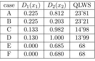
the QLWS in Eq. (1) is simplified as the rule exploited to represent numbers with a base-B positional system. By focusing for instance on a dummy two-objectives optimization (for whichp1= 1 andp2 = 0), and setting B = 100, let us analyse the value of the QLWS in Eq. (1) obtained by considering some mapping function results that we have simulated just for the sake of clearness and that are collected in Table 1. With particular reference to the first line of the table (case A), the QLWS (2381) is given by the term relevant to the high-priority target (2300 = 100×23) plus the term relevant to low-priority target (81). This means that, with reference to the 100 quantization levels adopted for the output of the mapping functions Dk(xk) by setting B = 100, we are 23 levels far from the fulfilment of the
high-priority target, and 81 levels far from the fulfilment of the low-priority target. Interestingly, this information is directly coded in the sequence of digits of the QLWS (23’81). In other words, splitting the digits of the QLWS values in groups of log10(B) allows the emphasis on one hand the priority levels in which the QLWS is divided and on the other hand how far each target is from its fulfilment. Note that in the case reported in the table,B = 100 and therefore log10(B) = 2; moreover, the digits groups are separated by the symbol.
To further show how the proposed QLWS in Eq. (1) handles items i) and ii) listed above, let us still focus on the dummy two-objectives optimization addressed above and analyse the values of the QLWS obtained by considering all the mapping function results collected in Table 1.
Table 1. Values of the QLWS for a two-objectives optimization.
case D1(x1) D2(x2) QLWS
A 0.225 0.812 23’81
B 0.225 0.203 23’21
C 0.133 0.982 14’98
D 0.130 1.000 13’99
E 0.000 0.685 68
F 0.000 0.680 68
From the results collected in the table we can can see:
• case A shows a QLWS greater than case B, since the high-priority target mapping is the same, but the low-priority target mapping is reduced;
• case D shows an even lower QLWS, since both target mappings are reduced; • in case E we have the satisfaction of the high-priority mapping;
• the QLWS of case F is equal to the QLWS of case E, even if the low-priority target is reduced because of a quantization effect induced by the ceiling function.
The dummy example reported above allows us also clarifying the role of B in the definition of the QLWS in Eq. (1). More specifically, a low value of B increases the quantization effect, namely, the QLWS becomes less sensitive to small variations of the mapping functionsDk(xk). On the other hand,
B cannot be too big; otherwise, the QLWS could become not sufficiently sensitive to a modification of a lower priority objective when the higher ones remain unchanged; moreover, we could be susceptible to the limited machine precision for the number representation.
Some additional considerations on the QLWS in Eq. (1) are now in order.
First, the ceiling function in Eq. (1) is not strictly required when we deal with the lowest priority target. So, hereafter in the paper the ceiling function for that term of the summation will be always dropped. This allows removing the quantization effect in the final convergence phase of the algorithm when, hopefully, all the higher priority targets are already satisfied.
Second, the proposed QLWS in Eq. (1) is not continuous due to the quantization effect introduced by the ceiling function. Accordingly, minimization of a so built GCF requires the exploitation of optimization methods that do not involve derivatives of the GCF itself. For instance, the proposed QLWS can be exploited by almost any evolutionary computation method as well as local minimization approaches like the Nelder-Mead simplex [11]. More generally, we can effectively exploit any previously used single-target minimization tool, provided that it does not require the calculation of the GCF derivatives.
Third, the proposed QLWS in Eq. (1) can be built in a simple and clear way: this represents a great advantage respect to other a-priori methods. As a comparison, when we use a weighted sum as defined in [1], we do not know the effect of a particular choice of the weights on the result of the optimization until we have several runs of the optimizer.
Finally, to properly handle the possible presence of targets with the same priority, we can generalize the expression of the QLWS in Eq. (1) as follows:
QLW S=
N
k=1
Bpkceil((B−ν
k)wkDk(xk)) (2)
whereνk is the number of targets having the same prioritypk, whereaswk is the weight for the target
associated to the optimization objective xk. In particular, the sum of the weights wk of targets having
the same priority must be equal to 1. In this way, in the QLWS in Eq. (2) we render the overall (maximum) contribution associated to theν terms with prioritypequal to the (maximum) contribution that we would have if the the same priorityp would be assigned to just one target. As matter of fact, use of Eq. (2) makes it possible the exploitation of the weights wk to give to different optimization
objectives the same priority with a slightly modified balance. By the way, this is an “advanced feature”, since we could simply implement a strict list of priorities by exploiting the QLWS in Eq. (1).
In the following sections we show the capability of the presented QLWS to handle various problems in antenna array synthesis.
3. SYNTHESIS OF A SPARSE LINEAR ARRAY
As an example of application of the proposed QLWS, in this section we address the calculation of the antennas positions and excitations in a sparse linear array.
should work as near as possible to their optimal condition. Accordingly, we are interested in minimizing the variation of the amplitude element’s excitations [13, 14].
For such a multi-objective problem we have to set the list of priorities among the targets. In particular, the maximum priority is assigned to the minimum inter-element constraint (which has to be greater than a given threshold). Then to the SLL (which has to be lower than a given threshold). Finally, the lowest priority is assigned to the reduction of the dynamic of the excitations (which should be as low as possible).
To translate these requirements within the QLWS in Eq. (1) it is convenient to recall the expression of the pattern of a linear array ofL elements:
F(u) =g(u)
L
=1
iejβxu (3)
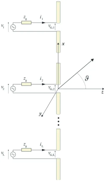
where the geometry depicted in Fig. 1 has been used. In particular, u = sin(θ), θ being the elevation angle of the observation point (see Fig. 1);x are the sorted abscissas of the element positions;λis the
free space wavelength; β = 2π/λ is the free space wavenumber; i are the excitations currents of the
elements;g(u) is the (co-polar) pattern of the array’s elements. It is stressed that the element factor has been supposed, just for the sake of simplicity, symmetric with respect to the array axis; furthermore, the array elements are supposed identical and equally oriented. It is also noted that in Eq. (3) we have neglected an inessential multiplicative constant.
In order to account for the possible presence of mutual coupling effects, the vector i = [i1, , iL] of
the excitation currents of the elements can be related to the vector of the excitations at the generators
v= [v1, , vL] by means of the following relationship:
v= (ZgId+Zm)i (4)
where Id is a (L, L) identity matrix, Zg the internal impedance of the generators (which are supposed
equal for all the radiating elements), and Zm the mutual coupling matrix [15].
The minimum inter-element distance of the array is:
d= min
∈2...Lx−x−1 (5)
The pattern SLL is given by:
SLL= 20 log10 max
|u|≥u0 |F(u)|
|F(0)| (6)
whereu0= sin(θ0),θ0 being the angle from which we want the SLL constraint to be satisfied. Finally, the dynamic of the excitations is defined as:
ρ= 20 log10 max
(|v|)
min
(|v|)
. (7)
In our example we consider a vertical array of L = 9 vertically aligned wire dipoles of length
lw = 0.48λ and diameter dw =λ/1000. Accordingly, the co-polar pattern g(u) of the array’s elements
is:
g(u) = cos(uβlw√/2)−cos(βlw/2)
1−u2 . (8)
where an inessential multiplicative constant has been neglected. It is also noted that the polarization of the radiated far-field is linear for all the directions.
With reference to the set of priorities listed above, for such an array we require that the minimum inter-element distance isλ/2 and that the maximum SLL is −20 dB forθ≥8◦.
According to the above definitions, the aforementioned priorities can be translated into the QLWS Eq. (1) using:
• N = 3, B= 103,L= 9 and u0 = sin(8◦);
• p1 = 3,D1(d) built as shown in Appendix, see (A2) withdmin= 0λ,dmax= 0.5λ;
• p2 = 2,D2(SLL) built as shown in Appendix, see (A1) with SLLmin =−20 dB, SLLmax= 0 dB; • p3 = 1,D3(ρ) built as shown in Appendix, see (A1) withρmin= 0, ρmax= 100.
As discussed in Section 2, the “ceiling” function of Eq. (1) is dropped for the lowest priority optimization objective.
It is important to underline that we could have considered other optimization parameters, like directivity or realized gain, in addition to the previous ones. Furthermore, regardless of the specific choices on the QLWS, one can decide to exploit the “most appropriate” optimization algorithm (provided that it can handle discontinuities in the cost function) as well as the “most appropriate” electromagnetic model for the specific problem object of the optimization, without any significant modifications of the QLWS itself. It is worth underlining that it could be possible to directly implement the QLWS in all full-wave solvers that have an optimizing function and allow editing a user defined global cost function. In particular, to account for the mutual coupling effects, we have used Eq. (4) by building the mutual coupling matrix Zm according to the closed form formulas in [15]. Furthermore, we have set
Zg = 50 Ω. This choice allows a very quick optimization of the antenna array but, as it will be shown
later, the accuracy of the closed form formulas is very satisfactory. Anyway, for different kind of antenna elements it could have been possible to use a full-wave software for the simulations, or a sophisticated hybrid method, but this is not essential to demonstrate the effectiveness of the QLWS.
the search space with respect to a standard evolutionary algorithms). The GA uses a population of 96 individuals, that are selected by means of tournaments of 3 individuals. The selected genes are then crossovered with random mapping, and the genes are mutated by means of Gaussian additive random variables. Finally, to avoid stagnation, random individuals are added to the population before the crossover. The termination of the algorithm is determined when the number of iterations reaches a chosen maximum (300).
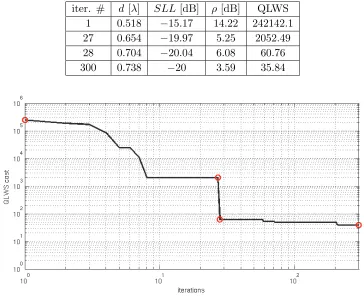
Fig. 2 shows the behaviour of the implemented QLWS as a function of the number of iterations. Moreover, we have picked up from the plotted curve some noticeable points, which are reported in Table 2. It can be seen that at iteration 1 we have QLWS = 242142.10 meaning that the minimum distance constraint is verified from the very first iteration (d = 0.518λ), but SLL = −15.17 dB and
ρ = 14.22 dB. This is not surprising; indeed, the positions of the radiating elements of the starting population are random, and it is not strange that at least one of the individuals of this starting population satisfies the first constraint. At iteration 27 we have QLWS = 2052.49, meaning that also the maximum SLL constraints is close to be verified. In fact, we have d= 0.654λ, SLL =−19.97 dB and ρ = 5.25 dB. At iteration 28 we have QLWS = 77.51, meaning that now also the maximum SLL constraints is verified: we have d = 0.704λ, SLL = −20.04 dB and ρ = 6.08 dB. From 27 to 28 the algorithm has “switched” its mode: in the first 28 iterations it was searching for a low SLL solution, now it is going to optimize for the excitation dynamic. At iteration 300, that is, the final one, we have QLWS = 35.84, d= 0.738λ, SLL=−20.00 dB and ρ = 3.59 dB, confirming that the algorithm in the final part has only worked to optimize for the dynamic of the excitations. The overall optimization took about 20 minutes on a i5-2320 personal computer.
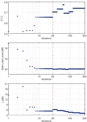
To achieve a better insight on the optimization process, in Fig. 3 we provide the values of all the optimization objectives as a function of the number of iterations. To this regard, we recall that
Table 2. Behaviour of the sparse array optimization objectives for some noticeable points of Fig. 2.
iter. # d[λ] SLL [dB] ρ[dB] QLWS
1 0.518 −15.17 14.22 242142.1
27 0.654 −19.97 5.25 2052.49
28 0.704 −20.04 6.08 60.76
300 0.738 −20 3.59 35.84
1 10 28 100 300 0.5
0.6 0.7 0.8
d [
λ
]
iterations
1 10 28 100 300
20 18 16
Side Lobe Level [dB]
iterations
1 10 28 100 300
3 6 9 12 15 18 21
ρ
[dB]
iterations
Figure 3. Behaviour of the optimization objectives as a function of the iterations. A vertical dashed red line marks some noticeable iterations detailed in Table 2.
the highest priority target (minimum allowable d) is verified from the first iteration. As for the two remaining targets (maximum allowable SLL and ρ, respectively), a vertical dashed line identifies two regions. In the left one the algorithm tries to achieve the desired SLL. Once this target is reached (that is, in correspondence of the dashed line), the algorithm tries to reduce the excitation’s dynamicρ, see the right region of the figure.
It is stressed that the use of the QLWS allowed the multi-objective optimization to work exactly as we wanted. In particular, the solutions with minimum inter-element distances lower than the chosen threshold are never used (because of their high cost). Then, the algorithm works for obtaining a solution that satisfies the SLL constraint (up to iteration 28). Finally, the algorithm works for reducing as much as possible the dynamic of the excitations. Note that the “switch” on what the algorithm does not requires the intervention of a human operator, since such information is already coded in the QLWS.
Figure 4. Obtained pattern for the sparse array of 9 elements calculated by means of the closed form formulas for the mutual coupling compared with a full-wave simulation.
Table 3. The parameters of the sparse array found.
x[λ] |a| ∠a [deg] |v| ∠v [deg]
1 0.000 0.0962 −11.292 10.651 −7.684 2 0.919 0.0957 −6.45 10.418 1.267 3 1.841 0.1239 −9.748 13.871 −3.545 4 2.663 0.1351 −11.585 15.705 −4.67 5 3.431 0.1337 −12.182 15.745 −4.97 6 4.258 0.1226 −9.551 14.663 −2.08 7 5.012 0.1038 −10.67 12.666 −0.663
8 5.75 0.0948 −1.76 11.318 6.708
9 6.705 0.0956 −9.819 10.651 −6.227
4. SYNTHESIS OF A SPARSE ISOPHORIC CIRCULAR ARRAY
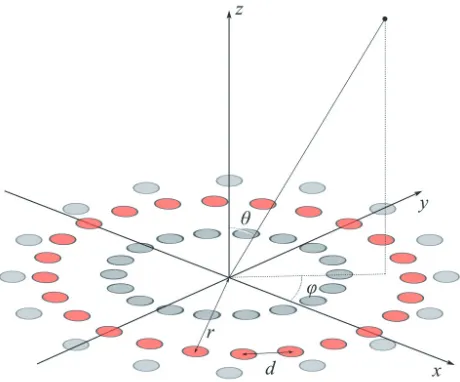
As a second example we move toward a planar geometry. In particular, we consider the synthesis of sparse circular isophoric (i.e., having constant input power for each antenna) arrays consisting of concentric rings (Fig. 5). Such an architecture is well suited for spatial applications [9].
Apart from an inessential multiplicative constant, the expression of the pattern of an isophoric sparse circular array consisting of concentric rings is [15]:
F(θ, ϕ) =g(θ, ϕ)
NR
m=1
nm−1
n=0
ejβrmsin(θ) cos
ϕ−ϕ(nm)
(9)
where θ and ϕ are the angular coordinates of the observation point according to the reference system depicted in Fig. 5). Furthermore,NR is the total number of rings;nm is the number of elements of the
m-th ring array; rm and ϕ(nm) = ψm + 2π(m−1)/nm represent, respectively, the radial and azimuth
coordinates of the n−th array element of the m-th ring (see Fig. 5). Finally, as in Eq. (3), λ and β
are the free space wavelength and wavenumber, respectively, andg(θ, ϕ) is the (co-polar) pattern of the array’s elements (which are supposed identical).
Figure 5. Circular array geometry.
sparse arrays. All of them aim at finding the optimal number of rings NR, set of radii rm, number of
feeds per ring nm and relative orientation ψm (m ∈ {1. . . NR}) of the antennas on the ring to achieve
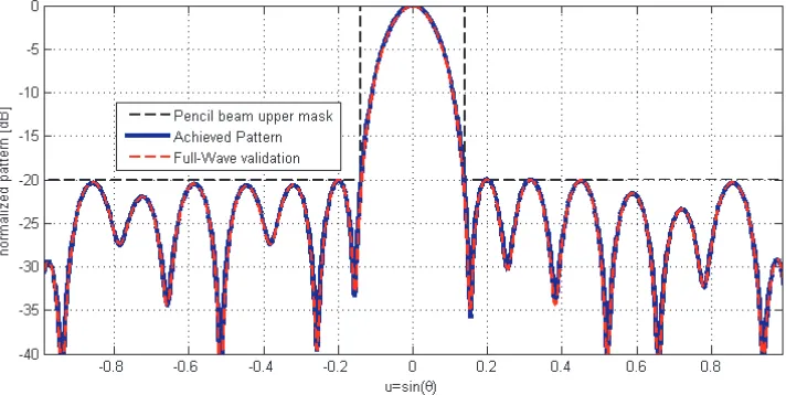
the desired pattern. In the following we show that the use of the QLWS allows the satisfaction of many concurrent constraints for this kind of synthesis. In particular, we focus on the radiation of a pencil beam pattern similar to that considered in [19], where the design of a sparse array for SATCOM applications is addressed. More specifically, the specifications of the desired antenna are the following: • the pattern must have a directivity, say DIR, greater than 41 dBi within the angular regionθ≤θEOC
beingθthe elevation angle of the observation point andθEOC = 0.325◦[deg] the Edge Of Coverage
(EOC) angle; calculated in this case with respect to the minimum EOC directivity, must be lower than−20 dB;
• the layout should not have radiating elements in the inner area of 10λ radius (in order to leave space for a secondary antenna), and the area occupation of the antenna should be lower than 55λ
radius;
• the number of overall employed elements should be as low as possible.
As shown in [6], for such kind of applications a proper dimension for the array element is on the order of 3λ. Thus, the mutual coupling effects on both the co-polar and cross-polar patterns radiated by the feeds [20–22] can be safely neglected during the synthesis. To better clarify this aspect, as preliminary step we analysed the relevance of the mutual coupling in the sparse array under analysis by carrying out a full-wave simulation with HFSS involving circularly polarized horns of 3λ diameter (namely, the dimension of the feeds that are used in the example of this paragraph); the height of the truncated cone of the horns is 4λ and the bottom section diameter is 0.6λ. In particular, we have evaluated the mutual coupling coefficient between two identical adjacent horns, finding a value of S21 lower than −45 dB; furthermore, we have compared the pattern of a horn in free space respect to the active element pattern [23] of the same horn surrounded by 6 adjacent horns closed on matched loads, as in Fig. 6 (a worst case scenario).
From Fig. 7 we can see that the co-polar component (left-handed circular polarization) is more than 25 dB higher than the cross polar component (right-handed circular polarization), in the angular region up to 8◦, which is the angular region covered by the Earth from satellite GEO orbit. Furthermore, the difference in the co-polar component directivity of the active element pattern with respect to the isolated horn is lower than 0.1 dB in the same region of interest.
Figure 6. Scheme of the circular horn surrounded by 6 other circular horns. The yellow horn is the active one, the cyan horns are closed on matched loads.
0 10 20 30 40 50 60 70 80 90
-20 -10 0 10 20
θ [deg]
Directivity [dBi]
isolated horn copolar pattern active element copolar pattern φ =0° active element copolar pattern φ=90° isolated horn crosspolar pattern active element crosspolar pattern φ=0° active element crosspolar pattern φ=90°
0 1 2 3 4 5 6 7 8 9 10
0 0.05 0.1 0.15 0.2
θ [deg]
Directivity [dB]
copolar pattern difference φ=0° copolar pattern difference φ=90°
(a)
(b)
Figure 7. (a) Directivity of the single horn and the active element pattern calculated considering 6 surrounding identical horns. (b) Difference of the directivity in the two cases.
Turning to the application of the proposed QLWS, as usual, we have to set the list of priorities among the targets. In particular, the SLL constraint has the maximum priority. With lower priority, the directivity constraint. Then, with the same priority, the two constraints on the minimum radius, (Rint) of the inner circular area and the maximum radius (Rext) of the overall array. Finally, with the lowest priority, the minimization of the number of elements (N tot).
Eq. (2) using:
• N = 5 and B = 103;
• p1 = 4, w1 = 1, ν1 = 1, D1(SLL) built as shown in Appendix, see (A1) with SLLmin =−20 dB,
SLLmax= 0 dB;
• p2 = 3, w2 = 1,ν2 = 1, D2(DIR) built as shown in Appendix, see (A2) with DIRmin = 36.0 dB,
DIRmax= 41.0 dB;
• p3 = 2, w3 = 0.5, ν3 = 2, D3(Rint) built as shown in Appendix, see (A2) with Rintmin = 0λ,
Rintmax= 10λ.
• p4 = 2, w4 = 0.5, ν4 = 2, D4(Rext) built as shown in Appendix, see (A1) with Rextmin = 55λ,
Rintmax= 65λ.
• p5 = 1, w4 = 1, ν4 = 1, D5(N tot) built as shown in Appendix, see (A1) with N totmin = 1,
N totmax= 999.
To solve this problem we have exploited the proposed QLWS cost function within the same evolutionary algorithm introduced in [9]. The implemented genetic algorithm employs tournament selection with 30 tournaments of 3 individuals. Each individual is characterized by a sorted vector of the radii rm and the number of feeds per ring nm is achieved by means of convex programming. The
algorithm is then stopped after a fixed number of iterations (2000). Since the relative orientations ψm
of the elements of the feeds on the ring have a very reduced impact on the final performances of the array [9], they are chosen just randomly.
To simplify the comparison we have employed the same number of rings NR = 9 of the reference
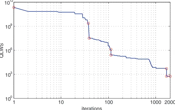
paper [19], and as feed we have considered the previously shown circularly polarized circular horn. In Fig. 8 the behaviour of the QLWS cost as a function of the number of iterations of the algorithm is shown. Moreover, in Table 4 some details on noticeable points of the plot of Fig. 8 are provided.
1 10 100 1000 2000
100 103 106 109 1012
QLWS
iterations
Figure 8. Minimum QLWS cost function behaviour for the optimization of a sparse circular array. The points marked with circles are detailed in Table 4.
1 10 39 114 200 1689 -20
-18 -16
Side Lobe Level [dB]
iterations
1 10 39 114 200 1689
40.5 41 41.5
Directivity [dBi]
iterations
1 10 39 114 200 1689
6 8 10
Internal radius [
λ
]
iterations
1 10 39 114 200 1689
55 57 59
External radius [
λ]
iterations
1 10 39 114 200 1689
500 550
Number of elements
iterations
Figure 9. Behaviour of the optimization objectives as a function of the iterations. Vertical dashed red lines mark some noticeable iterations detailed in Table 4.
It is finally noted that the overall synthesis took less than 45 minutes on a i5-2320 personal computer.
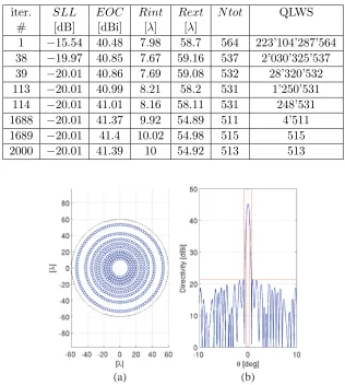
Table 4. Details on the points marked with circles of the plot of Fig. 8.
iter. SLL EOC Rint Rext N tot QLWS
# [dB] [dBi] [λ] [λ]
1 −15.54 40.48 7.98 58.7 564 223’104’287’564 38 −19.97 40.85 7.67 59.16 537 2’030’325’537
39 −20.01 40.86 7.69 59.08 532 28’320’532
113 −20.01 40.99 8.21 58.2 531 1’250’531
114 −20.01 41.01 8.16 58.11 531 248’531
1688 −20.01 41.37 9.92 54.89 511 4’511
1689 −20.01 41.4 10.02 54.98 515 515
2000 −20.01 41.39 10 54.92 513 513
(a) (b)
Figure 10. The synthesized sparse circular array. (a) Plot of the layout; (b) Superposition of the φ
cuts of the boresight directivity pattern (blue), power pattern mask (red).
Table 5. Parameters for the antenna layout of Fig. 10.
ring # rm [λ] nm ψm [rad]
1 11.505 24 0.131
2 14.515 30 0.105
3 17.587 36 0.087
4 20.642 43 0.073
5 25.794 53 0.059
6 30.070 62 0.051
7 35.126 71 0.044
8 42.359 86 0.037
5. CONCLUSIONS
In this work we have proposed the use of a novel cost function, the Quantized Lexicographic Weighted Sum (QLWS) in order to solve multi-criteria electromagnetic problems, handling the optimization constraints according to their priorities. The QLWS can be implemented in any optimization method, local or global, provided that such an algorithm can handle discontinuities in the cost function.
In order to show the effectiveness and flexibility of the proposed approach, we have applied the QLWS to two different antenna synthesis problems using two global search algorithms belonging to the family of evolutionary computation. In particular, in the first example we have obtained the elements’ excitations and positions of a sparse linear array, while in the second we have found the elements’ positions of a sparse planar isophoric array.
The two examples have shown that once the proposed QLWS is built according to the problem specifications, one can decide to exploit the “most appropriate” available optimization algorithm and electromagnetic model for the specific problem object of the optimization.
The presented results confirm the effectiveness of the proposed method that allows the translation of the specifications of the problem in a simple and direct way.
The examples chosen in this paper have been selected to clarify how the method works. However, the potential application of the proposed lexicographic approach is much more vast. In fact, the QLWS is particularly suitable for handling complex full wave simulations or multi-physics problems, for example involving electromagnetic, mechanical and/or thermal equations, with a large number of non-homogeneous optimization objectives. Indeed, the great advantage of the QLWS, compared to other multi-objective optimization approaches, is that it naturally matches the engineering way to handle complex projects, based on a list of priorities to be met in the system.
ACKNOWLEDGMENT
This work was partially developed within a research contract, signed in 2015, between the University of Naples “Parthenope” and the University of Cassino and Southern Lazio.
APPENDIX A. MAPPING FUNCTIONS EXAMPLES
In this appendix we provide some examples aimed at clarifying how we can build the mapping function
D(x) introduced in Section 2. In particular, we consider three single-objective cases picked up from classical antenna synthesis problems. As the first example, let us suppose that we are interested in minimizing a variable x (such as the side lobe level of a radiation pattern, or the insertion loss of a certain structure exploited to feed an array). More specifically, we need values of x lower than xmin; moreover, values greater thanxmax are equally considered bad. A mapping function capable of coding these requirements can be defined as follows:
D(x) = ⎧ ⎪ ⎨ ⎪ ⎩
1 ifx > xmax 0 ifx < xmin
x−xmin
xmax−xmin
otherwise
(A1)
Similarly, with the following mapping function
D(x) = ⎧ ⎪ ⎨ ⎪ ⎩
0 ifx > xmax 1 ifx < xmin
xmax−x
xmax−xmin
otherwise
(A2)
ofxgreater thanxmaxor lower thanxminare considered equally bad, we could use the following mapping function:
D(x) = ⎧ ⎪ ⎪ ⎪ ⎪ ⎪ ⎪ ⎨ ⎪ ⎪ ⎪ ⎪ ⎪ ⎪ ⎩
1 ifx > xmax 1 ifx < xmin
x−xd
xmax−xd
ifxd≤x≤xmax
xd−x
xd−xmin
ifxmin ≤x < xd
(A3)
REFERENCES
1. Ehrgott, M., Multicriteria Optimization, Springer Science & Business Media, 2006.
2. Marler, R. T. and J. S. Arora, “Survey of multi-objective optimization methods for engineering,”
Structural and Multidisciplinary Optimization, Vol. 26, No. 6, 369–395, 2004.
3. Yuan, X., Z. Li, D. Rodrigo, H. S. Mopidevi, O. Kaynar, L. Jofre, and B. A. Cetiner, “A parasitic layer-based reconfigurable antenna design by multi-objective optimization,”IEEE Transactions on Antennas and Propagation, Vol. 60, No. 6, 2690–2701, Jun. 2012.
4. Koziel, S. and S. Ogurtsov, “Multi-objective design of antennas using variable-fidelity simulations and surrogate models,” IEEE Transactions on Antennas and Propagation, Vol. 61, No. 12, 5931– 5939, Dec. 2013.
5. Goudos, S. K., K. A. Gotsis, K. Siakavara, E. E. Vafiadis, and J. N. Sahalos, “A multi-objective approach to subarrayed linear antenna arrays design based on memetic differential evolution,”IEEE Transactions on Antennas and Propagation, Vol. 61, No. 6, 3042–3052, Jun. 2013.
6. Bucci, O. M., T. Isernia, S. Perna, and D. Pinchera, “Isophoric sparse arrays ensuring global coverage in satellite communications,” IEEE Transactions on Antennas and Propagation, Vol. 62, No. 4, 1607–1618, Apr. 2014.
7. Jayasinghe, J. W., J. Anguera, D. N. Uduwawala, and A. And´ujar, “A multipurpose genetically engineered microstrip patch antennas: Bandwidth, gain, and polarization,”Microwave and Optical Technology Letters, Vol. 59, No. 4, 941–949, 2017.
8. Migliore, M. D., D. Pinchera, and F. Schettino, “A simple and robust adaptive parasitic antenna,”
IEEE Transactions on Antennas and Propagation, Vol. 53, No. 10, 3262–3272, Oct. 2005.
9. Bucci, O. M. and D. Pinchera, “A generalized hybrid approach for the synthesis of uniform amplitude pencil beam ring-arrays,” IEEE Transactions on Antennas and Propagation, Vol. 60, No. 1, 174–183, 2012.
10. Wolpert, D. H. and W. G. Macready, “No free lunch theorems for optimization,”IEEE Transactions on Evolutionary Computation, Vol. 1, No. 1, 67–82, 1997.
11. Nelder, J. A. and R. Mead, “A simplex method for function minimization,”The Computer Journal, Vol. 7, No. 4, 308–313, 1965.
12. Bucci, O. M., M. D’Urso, and T. Isernia, “Some facts and challenges in array antenna synthesis,”
19th International Conference on Applied Electromagnetics and Communications, 2007, ICECom 2007, 1–4, Sept. 2007.
13. Toso, G., C. Mangenot, and A. Roederer, “Sparse and thinned arrays for multiple beam satellite applications,”The Second European Conference on Antennas and Propagation, 2007, EuCAP 2007, 1–4, IET, 2007.
14. Anselmi, N., P. Rocca, M. Salucci, and A. Massa, “Optimisation of excitation tolerances for robust beamforming in linear arrays,” IET Microwaves, Antennas Propagation, Vol. 10, No. 2, 208–214, 2016.
15. Balanis, C. A.,Antenna Theory: Analysis and Design, John Wiley & Sons, 2016.
17. Weile, D. S. and E. Michielssen, “Genetic algorithm optimization applied to electromagnetics: A review,”IEEE Transactions on Antennas and Propagation, Vol. 45, No. 3, 343–353, 1997.
18. Bucci, O. M. and S. Perna, “A deterministic two dimensional density taper approach for fast design of uniform amplitude pencil beams arrays,” IEEE Transactions on Antennas and Propagation, Vol. 59, No. 8, 2852–2861, 2011.
20. Hamid, M., “Mutual coupling between sectoral horns side by side,”IEEE Transactions on Antennas and Propagation, Vol. 15, No. 3, 475–477, 1967.
21. Clarricoats, P., S. Tun, and C. Parini, “Effects of mutual coupling in conical horn arrays,” IEE Proceedings H, Microwaves, Optics and Antennas, Vol. 131, No. 3, 165–171, 1984.
22. Bencivenni, C., M. Ivashina, R. Maaskant, and J. Wettergren, “Synthesis of maximally sparse arrays using compressive sensing and full-wave analysis for global earth coverage applications,”
IEEE Transactions on Antennas and Propagation, Vol. 64, No. 11, 4873, 2016.
23. Pozar, D. M., “The active element pattern,” IEEE Transactions on Antennas and Propagation, Vol. 42, No. 8, 1176–1178, 1994.
24. Angeletti, P., G. Toso, and G. Ruggerini, “Array antennas with jointly optimized elements positions and dimensions Part II: Planar circular arrays,”IEEE Transactions on Antennas and Propagation, Vol. 62, No. 4, 1627–1639, 2014.