Western University Western University
Scholarship@Western
Scholarship@Western
Electronic Thesis and Dissertation Repository
12-17-2014 12:00 AM
Computing Intersection Multiplicity via Triangular Decomposition
Computing Intersection Multiplicity via Triangular Decomposition
Paul Vrbik
The University of Western Ontario Supervisor
Dr. Marc Moreno Maza
The University of Western Ontario Joint Supervisor Dr. Eric Schost
The University of Western Ontario Graduate Program in Computer Science
A thesis submitted in partial fulfillment of the requirements for the degree in Doctor of Philosophy
© Paul Vrbik 2014
Follow this and additional works at: https://ir.lib.uwo.ca/etd
Part of the Algebraic Geometry Commons, and the Theory and Algorithms Commons
Recommended Citation Recommended Citation
Vrbik, Paul, "Computing Intersection Multiplicity via Triangular Decomposition" (2014). Electronic Thesis and Dissertation Repository. 2631.
https://ir.lib.uwo.ca/etd/2631
This Dissertation/Thesis is brought to you for free and open access by Scholarship@Western. It has been accepted for inclusion in Electronic Thesis and Dissertation Repository by an authorized administrator of
Computing Intersection Multiplicity via Triangular Decomposition
(Thesis format: Monograph)
by
Paul Vrbik
Graduate Program in Computer Science
A thesis submitted in partial fulfillment of the requirements for the degree of
Doctor of Philosophy
The School of Graduate and Postdoctoral Studies The University of Western Ontario
London, Ontario, Canada
Abstract
Fulton’s algorithm is used to calculate the intersection multiplicity of two plane curves about a rational point. This work extends Fulton’s algorithm first to algebraic points (encoded by regular chains) and then, with some generic assumptions, to ℓmany hypersurfaces.
Out of necessity, we give a standard-basis free method (i.e. practically efficient method) for calculating tangent cones at points on curves.
Keywords. Algebraic geometry, Computer Algebra, Intersection Multi-plicity, Intersection Number, Fulton’s Algorithm, Tangent Cone.
For DLM — hero of listening.
Acknowledgments
I wish to thank. . .
My co-supervisors Dr. Marc Moreno Maza and Dr. ´Eric Schost who have spent a sensational amount of time and energy training me. For their patience, wisdom, and guidance I am deeply grateful.
Marc for choosing a good problem — the fact we were able to develop a comprehensive solution is a testament to his good judgement and intuition.
´
Eric for shaping my loose ideas into algorithms and my ‘proofs’ into proofs — I truly benefited from his extensive experience and keen eye.
My long-time friend Dr. Steffen Marcus. His role as our (very) pure mathematician consultant was critical for this work.
Dr. Michael Monagan for flying me out to Vancouver each summer and Roman Pearce for buying me dinner at every conference we have attended together.
The good people of ORCCA and the department’s support staff: thanks for putting up with me.
Contents
Abstract ii
Dedication iii
Acknowledgments iv
Table of Contents vii
0 Introduction 1
0.1 First Example . . . 2
0.2 Contributions . . . 3
0.3 Review of Literature . . . 5
0.4 Summary . . . 6
1 Ideals and Varieties 7 1.1 Polynomials . . . 7
1.1.1 Monomial Orderings . . . 8
1.1.2 Operations on Polynomials . . . 9
1.1.3 Polynomial Remainder Sequences . . . 11
1.1.4 Solving Polynomials . . . 13
1.2 Ideals and Varieties . . . 14
1.2.1 Varieties . . . 14
1.2.2 Ideals . . . 15
1.2.3 The Ideal Variety Correspondence . . . 16
1.2.4 Prime Ideals and Irreducible Varieties . . . 17
1.3 The Dimension of an Ideal . . . 18
2 Regular Chains 19
CONTENTS vi
2.1 Solving . . . 19
2.2 Triangular Sets . . . 21
2.2.1 Properties of Triangular Sets . . . 22
2.3 Regular Chains . . . 23
2.3.1 Shedding Bad Initials . . . 24
2.3.2 Specializing at Regular Chains . . . 26
2.4 Triangularization . . . 26
2.5 Splitting and the D5 Principle . . . 28
2.5.1 Regularize . . . 29
3 Intersection Multiplicity 32 3.1 Bivariate Intersection Multiplicity . . . 32
3.2 Fulton’s Properties . . . 35
3.3 Extending Fulton’s Properties . . . 37
4 Fulton’s Algorithm for Regular Chains 45 4.1 Descriptions . . . 45
4.2 Valuations . . . 47
4.3 Maximal Ideals . . . 49
4.4 Non-Splitting Case . . . 50
4.5 Splitting Case . . . 55
5 Tangent Cones 58 5.1 Singularities . . . 58
5.2 Homogeneous Components . . . 60
5.2.1 Classical Tangent Cone Definition . . . 62
5.2.2 Secants . . . 64
5.3 Tangent Cone Algorithm . . . 64
5.3.1 Equations of Tangent Cones . . . 71
5.3.2 Examples . . . 72
6 Extended Fulton’s Algorithm 77 6.1 Transversality . . . 77
6.2 Cylindrification . . . 81
CONTENTS vii
7 Experiments 89
7.1 Examples from literature . . . 92
7.1.1 Characteristic 101 . . . 92
7.1.2 Characteristic 962 592 769 . . . 95
7.1.3 Characteristic 0 . . . 99
7.2 Random Case Testing (Bivariate) . . . 103
7.3 Comparison to other systems . . . 106
Chapter 0
——
!——
Introduction
In algebraic geometry, the intersection multiplicity of two planar curves is an important quantity for it provides valuable information about the number of times these curves meet. This notion extends to the study of three surfaces and generalizes to ℓ hypersurfaces in an ℓ-dimensional space. It is useful to use this number to confirm all solutions are accounted for when solving a polynomial system, where the geometry may not be apparent.
As pointed out by Fulton in his “Intersection Theory” [14] the intersec-tion multiplicities of two plane curves satisfy a series of seven properties which uniquely define this number at each of the common points of these curves. Moreover, the proof of this (remarkable) fact is constructive, yield-ing (what we call) Fulton’s algorithm. This construction, however, is not given in spaces of dimension greater than two or at points that lie outside the (usually rational) coefficient field.
There are some barriers towards realizing a practical implementation of this algorithm. The main one is that computer algebra systems efficiently manipulate multivariate polynomials only when their coefficients are in the field of rational numbers or in a prime field. Nonetheless there are efficient algorithms [8] for decomposing algebraic varieties which rely only on field-operations and avoid explicit implementation of non-rational numbers.
In this manuscript: we extend Fulton’s algorithm to work at any point, rational or not; give algorithmic criteria for reducing the case of ℓ vari-ables to the (known) bivariate case; and (out of necessity) give a standard
first example 2
basis free algorithm for calculating tangent cones to make our reduction condition computational tractable to determine.
§
0.1 First Example
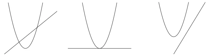
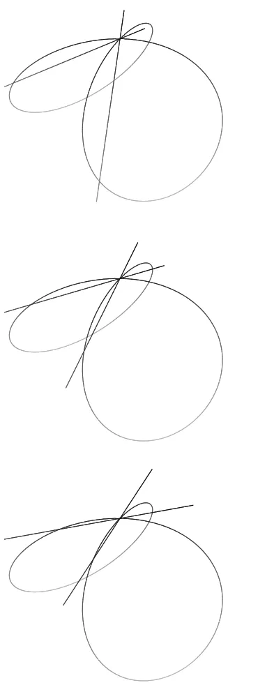
Consider the intersection of the parabola y = x2 with a line (y
− b) = m(x− a). The line and parabola meet at two distinct points except at the point p = (a, b) when m = 2a. Here the line is the tangent at p of the parabola and the intersection multiplicity of the two curves atpequals two.
Figure 1: The various intersections of a line and parabola corresponding to (resp.): two intersections of intersection multiplicity 1, one tangential tion of intersection multiplicity 2, and two complex intersections with intersec-tion multiplicity 1.
Within the pure-mathematical spectrum the intersection multiplicity provides insight into the local geometry of zero dimensional varieties. In this setting, the invariant is defined as the number of tangent lines at each point of intersection. The (practical) difficulty this introduces is the necessity to determine transversality with tangent cones at points with non-simple intersection (i.e. where more than one tangent is needed to locally approximate the zero-dimensional variety under study).
contributions 3
§
0.2 Contributions
There are three main contributions of this work:
We extend Fulton’s algorithm to work about zero-dimensional regu-lar chains which enables the calculation of intersection multiplicities at points in the algebraic closure of the coefficient field. Three procedures for calculating the intersection multiplicity of two planar curves are given. The first is designed to work at a point p, the second at an irreducible zero-dimensional regular chain, and the last at arbitrary zero-dimensional regular chains.
We also extend Fulton’s seven properties from two variables to ℓ+ 1 variables and provide an algorithmic criterion which allows for recursing the calculation of the intersection multiplicity in ℓ+ 1 variables toℓ variables. As a caveat our criterion involves the manipulation of a tangent cone which is often computationally prohibitive to obtain.
Fortunately, we give a standard-basis free method (i.e. practically ef-ficient method) for calculating tangent cones at points on curves. This, in itself, is an important contribution as there was no efficient method for calculating tangent cones before.
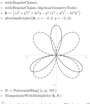
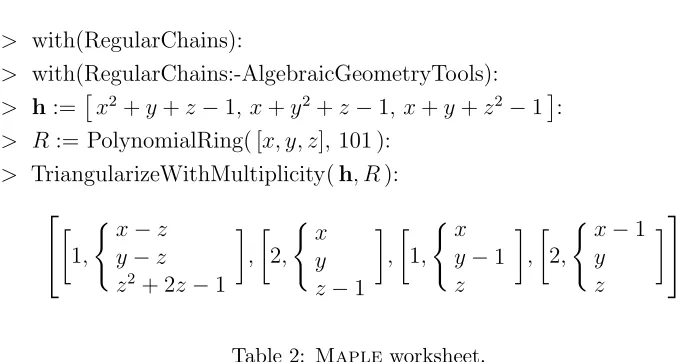
These algorithms have been implemented in theMaplelanguage as a sub-package of the RegularChains library. The Maple sessions in Table 1 and Table 2 illustrate computations with this package.
Consequently, we obtain a practical algorithm for computing intersec-tion multiplicities of zero-dimensional varieties. The novelty of our ap-proach is attributed to an important feature which is conducive to perfor-mance. Since we only require a triangular decomposition of a variety V — computed by any available method — we can operate without trying to ‘preserve’ any multiplicity information. Once V is decomposed, we are able to work ‘locally’ at each regular chain.
contributions 4
> with(RegularChains):
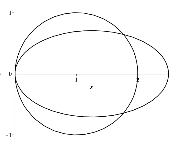
> with(RegularChains:-AlgebraicGeometryTools): > h:=!(x2+y2)2+ 3x2y
−y3,(x2+y2)3
−4x2y2":
> plots[implicitplot](h, x=−2..2, y=−2..2);
> R := PolynomialRing( [x, y], 101 ): > TriangularizeWithMultiplicity(h, R):
#$
1,%x−1 y+ 14
&
,$1,%x+ 1 y+ 14
&
,$1,%x−47 y−14
&
,$1,%x+ 47 y−14
&
,$14,%x y
&'
review of literature 5
> with(RegularChains):
> with(RegularChains:-AlgebraicGeometryTools): > h:=!x2+y+z
−1, x+y2+z
−1, x+y+z2 −1": > R := PolynomialRing( [x, y, z], 101 ):
> TriangularizeWithMultiplicity(h, R): ⎡
⎣ *
1,
+x−z y−z z2+ 2z
−1 , , * 2, +x y z−1
, ,
* 1,
+x y−1 z
, ,
* 2,
+x−1 y z
,⎤ ⎦
Table 2: Mapleworksheet.
We note that the question of computing intersection numbers in space of dimension greater than two is known to be highly challenging, even from a theoretical point of view, as noted in [34].
§
0.3 Review of Literature
The authors of [9] and [21] report algorithms with similar specifications to ours. The first is only applicable to the case of two input polynomials whereas [21] is not complete in the sense that it may not compute the intersection multiplicities of all regular chains in a triangular decomposition of the input system (even in the bivariate case).
summary 6
Finally the computer algebra systemsMagma andSingularprovide (resp.) IntersectionNumber [22, Example H84E6] and iMult [31] which calculate intersection multiplicities using (resp.) [16, Chapter I, Exercise 5.4] and standard basis techniques. However in both cases only the sum of the intersection multiplicities are counted and in fact some tangent lines may be counted twice, leading to over-counting.
§
0.4 Summary
This manuscript is organized as follows:
1. Chapter 1 is introduces the definitions and notations required to de-scribe the theory;
2. Chapter 2 is an overview of triangular sets, regular chains, and tri-angular decomposition;
3. Chapter 3 recounts a general introduction of intersection theory (in particular the intersection multiplicity) and contains the algorithm for computing intersection multiplicity at points from an algebraic closure;
4. Chapter 4 builds the extension to Fulton’s algorithm which works at irrational points;
5. Chapter 5 describes the tangent cone, its (classical) computation using standard basis, and our alternate method which uses triangular decomposition;
6. Chapter 6 contains our criterium for recursing the calculation of an intersection multiplicity in ℓ+ 1 variables toℓ variables; and finally
Chapter 1
——
!——
Ideals and Varieties
This chapter introduces the definitions and notations required to describe the theory in such a way to make implementation clear. The basic concepts and operations on rings, ideal, and varieties are defined as well as the notion of the dimension of an ideal and variety.
§
1.1 Polynomials
In what follows, for the entirety of this work, R is a ring,F is a field, and F is the algebraic closure ofF.
Polynomials are comprised of finite sums of monomials, which are in turn finite products of variables. So let N be the natural numbers and
x:={x0, . . . , xℓ}:ℓ∈N
be a finite set of variables.
An arbitrary (but finite) product of variables is amonomial.
Definition 1.1 (Monomials). Themonomials over variablesx:
[x] :=%xd0 0 · · ·x
dℓ
ℓ : (d0, . . . , dℓ)∈Nℓ+1
/
=0xd : d
∈Nℓ+11.
(Note: 1∈ [x] and 0̸∈[x].)
The product of a monomialmandcfrom the ringR(calledm’scoefficient)
is a term.
polynomials 8
Definition 1.2 (Terms). The terms with monomials from [x] and coeffi -cients from the ring R are given by
[x]R :={cm :c∈ R, m∈[x]}.
And finally, a finite sum of terms is a polynomial, the comprehensive set of which form a ring.
Definition 1.3 (Polynomial Ring). Polynomials with variablesx over the coefficient ring R:
R[x] :={2
t∈t
t :t⊆ [x]R and |t|<∞}.
Equivalent and more common representations of the polynomial ring are:
R[x] ={f0+· · ·+fs :f0, . . . , fs∈[x]R and s <∞}
and R[x] =3cαxα0 0 · · ·x
αℓ
ℓ forcα∈R.
§
Monomial Orderings
To impose some canonical form on our polynomials we strive to write terms in descending degree as in
5x3+ 2x2+ 7x+ 3.
The same can be done with arbitrary polynomials from R[x] provided all
but one variable is ‘demoted’ to the coefficient ring. (The subsequent one variable polynomial is said to be univariate.)
Example 1.1. The polynomial
xyz+y3+x3+x2z∈R[x, y, z]
re-written as a univariate polynomial in xwith descending degree:
x3+ (z)x2+ (yz)x+4y35
polynomials 9
The brackets on (z), (yz), and (y3) are meant to emphasize these
‘mono-mials’ are taken from the coefficient ring R[x, y].
Operations on univariate polynomials can be extended to multivariate polynomials provided the coefficients still form a ring. So, viewing multi-variate polynomials as unimulti-variate (in what we later call themain variable) is something we do frequently.
Generally, any total ordering ≺ of [x] (that is, an order satisfying
u≺ v and v≺u =⇒ u=v antisymmetry,
u≺v and v≺w =⇒ u≺w transitivity, and
[u≺v orv ≺u]≡ ⊤ totality
∀u, v, w ∈ [x]) is a monomial ordering when the ordering respects multi-plication and has 1 ordered least.
Definition 1.4 (Monomial ordering). Let u, v and w be monomials from [x] and ≻ : [x]→{⊤,⊥} be an ordering. The predicate ≻ is a monomial ordering when ≻ is a total ordering and
1. ∀w∈[x]; u≻v =⇒ uw≻vw, and
2. ∀u∈[x]; u≻1.
(As with the degree function we extend monomial orderings to terms by ignoring their coefficients.)
§
Operations on Polynomials
Definition 1.5 (deg). Thetotal degree of
1. a monomialxd0 0 · · ·x
dℓ
ℓ ∈[x] is
deg(xd0 0 · · ·xd
ℓ
ℓ ) :=d0+· · ·+dℓ;
2. a term cm∈[x]R such that c̸= 0 is
polynomials 10
3. a polynomial c0m0+· · ·+csms with mi ̸=mj and ci̸= 0 is
deg(c0m0+· · ·+csms) := max(deg(c0m0), . . . ,deg(csms)),
and following convention deg(0) :=−∞.
Example 1.2. In R[x, y, z]
deg4x3+y2+xy2z5= max4deg4x35, deg4y25,deg4x2yz55= 4.
We may also take the degree of a polynomialh∈R inxfor anyx∈ x.
This is simply the total degree ofhwhen taken as univariate in x. Denote this value by degx(h).
Example 1.3. h=x3+y2+xy2z
∈ R[x, y, z] has deg
x(h) = 3, degy(h) =
2, and degz(h) = 1.
Let us devote some notation for deconstructing and identifying the pieces of a polynomial.
Definition 1.6. Assume c0, . . . , cs∈ R−{0}, {m0, . . . , ms}⊆[x], m∈
[x], and f =c0m0+· · ·+csms∈ R[x].Let
1. terms(f) :={c0m0, . . . , csms}be the terms off,
2. monos(f) :={m0, . . . , ms}be the monomials of f, and
3. indets(m) := 0x∈ x: x66m1 be the indeterminates of a monomial m, and
4. indets(f) :=∪(indets(m) :m∈ monos(f)) be the indeterminates of the polynomial f.
Example 1.4. Letf =x3+2y2+3xy2zthen terms(f) ={x3,2y2,3xy2z},
monos(f) ={x3, y2, xy2z
},and indets(f) ={x, y , z}.
polynomials 11
Definition 1.7 (Leading Term). The leading term and leading monomial of a polynomialf ∈R[x] with respect to a monomial ordering ≻are given
by
ℓt(f) := max
≻ (t :t∈terms(f)) and ℓm(f) := max≻ (m: m∈ monos(f))
and the leading coefficient is
ℓc(f) := ℓt(f)
ℓm(f).
Example 1.5. Let f = x3 + 2y2+ 3xy2z be taken univariate in y with
coefficients fromR[x, z], that is y ≻x≻z, then
ℓt(f) = 2y2+ 3xy2z, ℓm(f) =y2, and ℓc(f) = 3xz+ 2.
§
Polynomial Remainder Sequences
We enumerate the basic polynomial remainder sequences.
Proposition 1.1. Let F be a field and g a nonzero polynomial in F[x].
For any f ∈ F[x] there areunique q, r∈ F[x] such that
f =q·g+r: degx(r)<degx(g).
Proof. See [11, Ch. 1 §5 Proposition 2.] where the division algorithm is outlined.
Definition 1.8 (Quotient and Remainder). The polynomialsq andrfrom Proposition 1.1 are called the quotient and remainder and are denoted by quo(f, g;x) and rem(f, g;x). They satisfy
polynomials 12
Notation (French long division). Let f, g, q, r∈F[x] then
f g
r q ⇐⇒
f =qm+r and deg(r)<deg.(m)
We sometimes require that F is the fraction field of a domain R;
for instance, R may be the polynomial ring Q[y], and F is the rational
function field Q(y). In this case, even if f and g are in R[x], the quotient
and remainder may lie in F[x].
For instance, letf =x4+ 1 and g =xy2+ 1 and note
f = x
3y6
−x2y4+xy2 −1
y8 ·g+
y8 −1 y8
where thereby
rem(f, g;x) = y
8 −1
y8 and quo(f, g;x) =
x3y6
−x2y4+xy2 −1
y8 .
A premultiplication can be done to preclude this possibility. We call the quotient and remainder calculated using premultiplications the pseudo-remainder and pseudo-quotient.
Proposition 1.2. Let f, g ∈ R[x] and let x ∈ x. Assume deg
x(f) <
degx(g) and g̸= 0. There areunique q ∈ R[x] andr∈ ⟨f, g⟩such that
m·f =q·h+r: degx(r)<degx(b)
where m=ℓcx(g)
degx(f)−degx(g)+1
Proof. See [11, Ch. 6§6 Proposition 1] where the pseudo-division algorithm is outlined.
Definition 1.9 (Pseudo-quotient and Pseudo-Remainder). Take the set-tings of Proposition 1.2. The polynomial r is called thepseudo-remainder in xand is denoted by prem(f, g; x). Thus
polynomials 13
where m=ℓcx(g)
degx(f)−degx(g)+1.
Example 1.6 (Pseudo-Remainder). Let f = x4+ 1 an g = xy2+ 1 and
note
4
y35·f =4xy2−y5·g+4y3−y5.
Thus prem(f, g;x) = (y3 −y).
§
Solving Polynomials
Polynomials definepolynomial mappingsfromaffine spacesintobase fields.1
Definition 1.10 (Affine Space). ForF a field,
Aℓ+1(F) :=F ×· · ·×F
7 89 :
ℓ+1-times
is called anaffine space.
For these mappings we adopt the familiar function notation. That is, when f ∈ F[x] and p= (p0, . . . , pℓ)∈ Aℓ+1(F) we take
f(p) :=f(p0, . . . , pℓ)
and let a polynomial map be given by the following.
Definition 1.11 (Polynomial Mapping). ForF a field andf ∈F[x], the
polynomial map given byf is
f : Aℓ+1(F)→F
p3→f(p).
Recall thekernel of a mapping is the subset of its domain which maps to zero. Solving a polynomial typically means deducing some or perhaps all of this kernel (also called the nullspace).
ideals and varieties 14
Definition 1.12 (Kernel). Let F be a field and f ∈F[x]. Let
ker(f) :=0p∈ Aℓ+1(F) :f(p) = 01.
Importantly, the kernel depends on the coefficient field. For instance f = (x2−2)(x2+ 1)∈F[x] can have zero, two, or four roots:
R ker(f)
Q ∅
R 0±√21
C 0±√2, ±i1 .
§
1.2 Ideals and Varieties
Much in the same way vector spaces are comprised of linear combinations of vectors, ideals are comprised of polynomial combinations of polynomials. They were first introduced by Richard Dedekind in 1876 as a generalization of ideal numbers [33].
Varieties arise as the kernel of these ideals and correspond to sets of points where the polynomials of the ideal vanish (i.e. become zero) si-multaneously. It is important that ideals are representable by computers while simultaneously representing infinitely large kernels. The broader ideal/variety correspondence allows for the conversion between geometric and algebraic points of view.
§
Varieties
Any subset of affine space which is the solution set of a system of poly-nomials is called a variety. A variety can be viewed as a function from
P(F[x]) (powerset of A) to Aℓ+1(F) which computes the set of points
where a finite set of polynomials vanish simultaneously:
ideals and varieties 15
This is the natural way of extending the kernel to that of systems of poly-nomials.
Definition 1.13 (Variety). Let f = {f0, . . . , fs} ⊆ F[x], for F a field,
and
V(f0, . . . , fs) := ker(f0)∩· · ·∩ker(fs).
V ⊆Aℓ+1(F) is called a variety when
∃f ⊆F[x] : V =V(f).
Example 1.7. Let f ={y−x2, y
−x}⊆ F[x, y] (the parabola and line
through the origin).
V4y−x2, y−x5= ker4y−x25∩ker(y−x)
=04p, p25 : p∈F1∩{(p, p) : p∈ F}
={(0,0),{1,1}}.
It is these varieties we wish to encode, and their points/elements we wish to classify.
§
Ideals
Observe ker : F[x]→Aℓ+1(F) isnot injective; there can be many (if not
infinitely many) polynomials with equivalent kernel:
ker(x−1) = ker(2x−2) = ker(3x−3) =· · ·={1}.
Not only this, we also require polynomials whose kernels inlude {1}.
Definition 1.14 (Ideal). Let I ⊆F[x]. I is anideal when
1. 0∈I,
2. f, g ∈I =⇒ f +g ∈I,
ideals and varieties 16
Definition 1.15 (Ideal Brackets). Let V ⊆ Aℓ+1(F) and I(V), the ideal
defined by V, be the set of all polynomials which vanish onV:
I(V) :={f ∈F[x] : V ⊆ker(f)}.
We use ideal brackets to represent these infinite sets. That is when f ⊆
F[x]:
⟨f⟩:=0 2
f∈f
cff :cf ∈F[x]
1 .
Proposition 1.3. For any f = {f0, . . . , fℓ} ⊆ F[x] we have ⟨f⟩ is an
ideal.
Proof. See [11, Ch. 1 §4 Lemma 1.].
For more on Ideals, Varieties, and Algorithms see [11].
§
The Ideal Variety Correspondence
The correspondence between varieties and ideals is important as it trans-lates problems of geometry into problems of algebra. The practical upshot of this is an encoding of geometric problems with objects that can be ma-nipulated with computers. Hilbert’s Nullstellensatz (German for “theorem of zeros” or more literally “zero-locus-theorem”) along with its weak and strong versions gives the precise relationship between algebra and geome-try.
Theorem 1.1 (Hilbert’s Nullstellensatz). Let f ⊆F[x] then
f ∈ I(V(f)) ⇐⇒ ∃m∈ N>0 :fm ∈ ⟨f⟩
Proof. [10, Ch. 4 §1 Theorem 1].
Whenfm
ideals and varieties 17
Definition 1.16(Radical). Letf ⊆F[x] and⟨f⟩be an ideal. Theradical
of ⟨f⟩is given as follows. ;
⟨f⟩:=0f : ∃m∈N>0;fm
∈ ⟨f⟩1
This enables us to write the Strong Nullstellensatz which states the ideal-variety correspondence is exact for radical ideals.
Theorem 1.2 (Strong Nullstellensatz). Let f ⊆F[x] then
I(V(⟨f⟩)) =;⟨f⟩.
Proof. [10, Ch. 4 §2 Theorem 6].
§
Prime Ideals and Irreducible Varieties
Definition 1.17 (Irreducible Variety). A variety V is irreducible if and only if when V =V0∪V1 then either V =V0 orV =V1.
For instanceV(xz, yz) isnotan irreducible variety becauseV(xz, yz) = V(x) ∪ V(z, y). Whereas the variety V(y−x2, z
−x3) is irreducible,
though this takes some work to prove. The key is to move from a geo-metric point of view to an algebraic one. This transformation leads to the notion of prime ideals which correspond to irreducible varieties.
Definition 1.18 (Prime Ideal). An ideal ⟨f⟩ofF[x] isprime if whenever
gh∈ ⟨f⟩theng ∈ ⟨f⟩or h∈ ⟨f⟩.
Proposition 1.4. Let V be an affine variety ofAℓ+14F5. V is irreducible
if and only if I(V) is prime ideal.
Proof. See [11, Ch. 4 §5 Proposition 3].
When working over an algebraically closed fieldF then the correspondence
between prime ideals and irreducible varieties is one-to-one.
the dimension of an ideal 18
Definition 1.19 (Maximal Ideal). Let f ⊆ F[x] with ⟨f⟩ ̸= F[x]. The
ideal ⟨f⟩ is maximal when for any g ⊆ F[x] where ⟨f⟩ ⊆ ⟨g⟩ either
⟨f⟩=⟨g⟩or⟨g⟩=F[x].
Importantly, any ideal of the form⟨x−p⟩=⟨x0−p0, . . . , xℓ−pℓ⟩is
maximal in F[x] (e.g. ⟨x−2, y−4⟩is maximal in F[x]).
§
1.3 The Dimension of an Ideal
Hilbert’s insight was characterizing the dimension of an ideal by the number of monomialsnot in the ideal (i.e. in the ideals complement) [11, Ch. 9§3]. This number is given by the so-calledHilbert Polynomial whose degree is already a definition for the dimension of a variety. Crucially, the mono-mial ideal⟨ℓt(h: h∈ ⟨h⟩)⟩has the same Hilbert Polynomial as⟨h⟩when the leading terms are taken with a graded monomial ordering (e.g. one that orders by total degree first and breaks ties somehow).
However, for our purposes it is sufficient to take [11, Ch. 9 §5 Corol-lary 3.] as definition for dimension.
Definition 1.20. Let V ⊆ Aℓ+1(F) be an affine variety and assume
I(V) ⊆ F[x]. The dimension of V is given by the largest (by
cardi-nality) y ⊆ x satisfying I(V)∩F[y] = {0}. That is to say, there are no
polynomials in I(V) with variables in y other than the zero polynomial.
The Zariski closure of a subset S ⊆ Aℓ+1(F) is the smallest (by set
inclusion) affine variety V(h) :h ⊆ F[x] which is a superset to it. S denotes the Zariski closure ofS andV(I(S)) =S.
Geometrically, the intersection I(V)∩F[y] is {0} only when the
Chapter 2
——
!——
Regular Chains
The subsequent chapter develops the notion of a triangular set and regular chain from the basic goal of ‘solving’ a system of polynomials — in fact, even the idea of solving requires consideration. Among the options for encoding the solutions are Gr¨obner basis, triangular sets, and (of course) regular chains. The utility of using regular chains is that they satisfy conditions of algorithmic importance. In particular, using regular chains enables the exploitation of efficient “splitting algorithms” [6].
Triangular sets, but more specifically their specialization into regular chains, are the principal objects of study of this work. They are critically important to computer algebra systems for their part in solving systems of polynomials and cylindrical algebraic decomposition.
See [4, 17, 36] for a general overview of the theory of triangular sets and regular chains.
§
2.1 Solving
‘Solving’ a system of polynomials, say h ⊆ F[x] for F a field, means
different things in different contexts. In each case however the goal is the same: encode the zeros of the polynomial system somehow.
For proofs, one typically wants either aprimary decomposition of ⟨h⟩ or a unique irreducible decomposition ofV(h). Though such a decomposi-tion can be desirable, computing them is akin to multivariate factorizadecomposi-tion
solving 20
which is computationally difficult. Additionally, these decompositions may not even be helpful for explicitly constructing points in V(h) and are not unique [15].
Example 2.1. Leth={x2+y+z
−1, x+y2+z
−1, x+y+z2
−1}⊆
F[x]. A primary decomposition of ⟨h⟩ is given by
⟨h′0⟩=<z−1, z2+x+y−1, x+y2+z−1, x2+y+z−1=,
⟨h′
1⟩=
<
z2+ 2z
−1, z2+x+y
−1, x+y2+z
−1, x2+y+z −1=,
⟨h′2⟩=
<
y, z, z2+x+y−1, x+y2+z−1, x2+y+z−1=,
⟨h′3⟩=
<
z, y−1, z2+x+y−11, x+y2+z−1, x2+y+z−1=,
where ⟨h⟩=⟨h′
0⟩ ∩· · ·∩ ⟨h′3⟩.
Note that the bad shape of these ideals (as produced by Maple) makes them unsuitable for back substitution.
An alternative is to use Gr¨obner bases. Buchberger’s algorithm allows for the computation of g ⊆ F[x] such that ⟨g⟩ = ⟨h⟩ and (crucially)
⟨ℓt(h) :h∈ ⟨h⟩⟩ = ⟨ℓt(g) : g∈ g⟩ for an arbitrary monomial ordering. Moreover, when reduced, these Gr¨obner bases are unique representations of the ideal.
Provided the basis is over a lexical monomial ordering, g satisfies the elimination condition that ⟨g⟩ ∩F[xn+1, . . . , xℓ] is a Gr¨obner basis of
the n-th elimination ideal. This property allows for a Gaussian-like back substitution.
Example 2.2. Leth={x2+y+z
−1, x+y2+z
−1, x+y+z2
−1}⊆
F[x, y, z]. A Gr¨obner basis of ⟨h⟩is
{z2+x+y−1, y2
−z2
−y+z, z4+ 2yz2−z2,
z6−4z4+ 4z3−z2}.
triangular sets 21
roots of y2 −z2
−y+z and z4+ 2yz2
−z2 simultaneously for some z ∈
V(z6
−4z4+ 4z3 −z2).
A third option and our preference is to use triangular decomposition. These decompositions are comparable to ‘minimal’ factorizations in the sense that only as many factors as necessary are calculated.
§
2.2 Triangular Sets
Intuitively, triangular sets are comprised of polynomials with mutually dif-ferent leading terms. The practical consequence of this isback substitution as it allows us to eliminate variables from the systems one by one. Reg-ular chains emerge by enforcing increasingly stronger conditions on these triangular sets.
Definition 2.1 (Main Variable). Let ≻ be an ordering of x. The main variable of a term t ∈ [x]F, and by extension a polynomial f ∈ F[x], is
given recursively
mvar(t) := max
≻ (v : v∈indets(t)),
mvar(f) := max
≻ (mvar(t) :t∈ terms(f)).
Definition 2.2 (Triangular Set). A set of polynomials with mutually dif-ferent main variable is a triangular set. Let T(F[x]) denote the class of
triangular sets ofF[x], then
f△∈ T(F[x]) ⇐⇒ ∀Defn. g, h∈f△ :g ̸=h; mvar(g)̸= mvar(h),
triangular sets 22
Example 2.3. A square triangular set ofF[x≺y ≺z≺t].
f△ = ⎧ ⎪ ⎪ ⎪ ⎪ ⎪ ⎨ ⎪ ⎪ ⎪ ⎪ ⎪ ⎩
(yz−1)t+y2
∈F[x, y, z, t]
xz2
−2yz+ 1 ∈F[x, y, z]
(x−1)y2
−x ∈F[x, y]
(x−1)(x+ 1) ∈F[x].
The shape of the polynomial rings as written form a triangle—the motiva-tion for the name “triangular sets.”
Triangular sets and regular chains are recursive so notation for breaking triangular sets into the ‘top’ and ‘bottom’ is prudent.
Notation. When f△∈T(F[x]) let
f⊤
△ := maxmvar(f : f ∈ f△), f
↑
△ :=f△−{f⊥△},
f△↓ :=f△−{f⊤△}, f⊥△:= min
mvar(f : f ∈ f△).
Note {f⊤△}∪f△↓ =f△↑ ∪{f⊥△}=f△.
§
Properties of Triangular Sets
The history of triangular sets dates back to at least 1932 when Joseph Fels Ritt demonstrated one can compute a triangular set equivalent to a given irreducible variety [7].
Let us first define the Iterated Pseudo-remainder.
Definition 2.3 (Iterated Pseudo-remainder). Let h ∈ F[x] and f△ ∈
T(F[x]) be a triangular set. The iterated pseudo-remainder is given
(re-cursively) by
prem∗(h, ∅; ∅) :=h,
prem∗(h, f△; x) := prem∗( prem(h, f⊤△;xℓ), f
↓
△;x
↓ ).
regular chains 23
Theorem 2.1 (Ritt, 1932). For anyh⊆ F[x] such that V(h) is an
irre-ducible variety one can construct a triangular setf△∈ T(F[x]) satisfying
∀h∈ ⟨h⟩; prem∗(h, f
△;x) = 0.
A set given by Theorem 2.1 is called a Ritt characteristic set and the utility of this construction is that it enables an ideal membership test on h.
Because irreducible components are often difficult to calculate, Wen-Tsun Wu in 1987 devised a method for computing triangular sets for ar-bitrary varieties [37]. Such sets are called Wu characteristic sets and can be calculated using fully Gr¨obner basis free methods [3].
Theorem 2.2(Wu, 1987).For anyh⊆F[x] one can compute a triangular
set f△ ⊆ ⟨h⟩such that
∀h∈h; prem∗(h, f
△; x) = 0.
Although certainly more widely applicable, Wu’s method cannot detect empty varieties. Empty varieties are those corresponding to polynomial systems with no solutions. The stronger restrictions imposed on triangular sets make them regular chains.
§
2.3 Regular Chains
Being a triangular set, despite having the right shape, provides no as-surance to back substitution being “well behaved.” In Example 2.3 for instance, substituting x = 1 into (x−1)y2
regular chains 24
§
Shedding Bad Initials
When a leading coefficient vanishes so doe, more disastrously, the leading term. Geometrically, shedding these bad substitution points simply means removing points from the variety where leading coefficients (or initials) vanish.
Definition 2.4 (Initial). The initial off ∈F[x] is the leading coefficient
of f when taken as univariate in its main variable.
init(f) := lcoeffmvar(f)(f).
Thequasi-component of a regular chain f△ corresponds to the removal of points where an initial of some f ∈ f△ vanishes.
Definition 2.5 (Quasi Component). Let f△∈T(F[x]), then
W(f△) :=V(f△)−VBCinit(f) : f∈f△D
is called the quasi component off△.
Algebraically removing bad initials from an ideal is less obvious. Here we must remove initials which are zero divisors modulo a ‘chain’ of regular chains. The saturation ideal, as it turns out, does this. Saturating an ideal has the desired effect of algebraically shedding bad initials.
Definition 2.6 (Colon Ideal). Let f,g⊆ F[x].
⟨f⟩:⟨g⟩:={h :∀g∈g; hg∈ ⟨f⟩}.
Definition 2.7 (Saturation Ideal). Let f△ ∈T(F[x]) and the product of
the initials be
init(f△) :=C(init(f) : f ∈f△).
The saturation off△ is the ideal
regular chains 25
In other words, f ∈ ⟨sat(f△)⟩ ⇐⇒ ∃Defn. n∈N>0 : init(f
△)nf ∈ ⟨f△⟩.
Notice saturating an ideal may make it larger.
Example 2.4. Let f△ = ⎧ ⎨ ⎩
zx+t
ty+z ∈
T(F[x, y, z, t])
⟨f△⟩=⟨z, t⟩ ∩ ⟨−xy+ 1, ty+z⟩, and
⟨sat(f△)⟩=⟨1−xy, ty+z⟩.
It is well known that the quasi-component and saturation ideal are related in the following manner [10].
Theorem 2.3. Let f△ ∈ T(F[x]) and W(f△) be the Zariski closure of
quasi-component of f△. Then
W(f△) =V(⟨sat(f△)⟩).
And finally, aregular chain is a triangular set whose top is regular (i.e. not a zero-divisor) modulo its bottom.
Definition 2.8 (Regular Element). Let f ∈ F[x], f ⊆ F[x], and U⟨f⟩ denote the set of regular elements among F[x]/⟨f⟩. Then
f ∈U⟨f⟩ ⇐⇒ ∀Defn. g ∈F[x]; f g≡ 0 mod⟨f⟩ =⇒ g≡ 0 mod⟨f⟩.
Moreover, let f ̸∈ U⟨f⟩be called a zero-divisor.
Definition 2.9(Regular Chain). Denote byTreg(F[x]) the class of regular
chains of F[x] and let Treg(F[x])⊆T(F[x]). Then
f△ ∈Treg(F[x]) Defn. ⇐⇒
⎧ ⎨ ⎩
f△=∅, or
f△↓ ∈Treg(F[x]) and init(f△⊤)∈ U⟨f△↓⟩.
triangularization 26
Proposition 2.1. Whenf△∈Treg(F[x]) the dimension ofW(f△) is given
by
dimW(f△) =ℓ+ 1−|f△|.
Proof. See [35].
§
Specializing at Regular Chains
When working over the complex numbers for instance specialization at maximal ideals corresponds to evaluation,
x2+ymod⟨x−1, y−2⟩= x2+y66x=1, y=2= 3
whereas more arbitrary ideals specialize at algebraic points
x2−4 mod<x2−2== x2−466x=±√
2 =−2
and so naturally at complex points as well
x4mod<x2+ 1== x466x=±√
−1= 1.
In any case, “modding out” a polynomial g by some ideal ⟨f⟩ has the effect ofsimultaneously evaluatingg at each point ofV(f). Thus, modular images can be (and are) used instead of explicit function evaluation.
§
2.4 Triangularization
In general there are two ways to decompose ⟨h⟩into regular chains. One can either describe the generic points of the ideal (a Kalkbrenner decom-position) or all the zeros of the corresponding variety (a Lazard decomposi-tion). There are various algorithms available for triangular decompositions in either sense.
triangularization 27
Theorem 2.4 (Kalkbrenner Decomposition). For anyh⊆F[x] there are
regular chains {f△,0, . . . ,f△, e}⊆Treg(F[x]) such that
;
⟨h⟩=;⟨sat(f△,0)⟩ ∩· · ·∩
;
⟨sat(f△, r)⟩
wheree∈ Nand, using the Ideal-Variety correspondence and Theorem 2.3, we also have
V(h) =W(f△,0)∪· · ·∪W(f△, e).
Additionally, there is an algorithm for computing a Kalkbrenner de-composition. We take this algorithm as black-box and simply let △(h) be the computed triangularization.
Definition 2.10 (Triangularize). For any idealh an ideal ofF[x] let the
triangularization of h be a mapping from the ideals of F[x] into sets of
regular chains fromF[x] given by
△ :P(F[x])→P(Treg(F[x]))
⟨h⟩ 3→{f△,0, . . . , f△, e} :V(h) =W(f△,0)∪· · ·∪W(f△, e).
where r∈N.
Moreover, Moreno Maza and Wang (simultaneously) in 2000 [32][28] gave the following guarantee regarding the decomposition of varieties into a disjoint union of quasi-components independent of the Zariski closure.
Theorem 2.5 (Lazard Decomposition). For any h⊆ F[x] there are
reg-ular chains {f△,0, . . . ,f△, r}⊆Treg(F[x]) such that
V(h) =W(f△,0)8· · ·8W(f△, e)
where 8 is the disjoint union and r∈N.
splitting and the d5 principle 28
Because Kalkbrenner decompositions are typically faster than Lazard decompositions, in practice the former is the default setting when using theTriangularizecommand in Maple. In particular, this is the case for our algorithms.[23]
Example 2.5. Leth={x2+y+z
−1, x+y2+z
−1, x+y+z2
−1}⊆
F[x]. A Kalkbrenner decomposition of⟨h⟩is given by
△(h) = % ⎧ ⎪ ⎪ ⎪ ⎨ ⎪ ⎪ ⎪ ⎩
x−z
y−z
z2+ 2z −1 , ⎧ ⎪ ⎪ ⎪ ⎨ ⎪ ⎪ ⎪ ⎩ x y
z−1 , ⎧ ⎪ ⎪ ⎪ ⎨ ⎪ ⎪ ⎪ ⎩ x
y−1
z , ⎧ ⎪ ⎪ ⎪ ⎨ ⎪ ⎪ ⎪ ⎩
x−1
y
z
/
§
2.5 Splitting and the D5 Principle
The intuition behind triangular decomposition algorithms is to “follow the one variable polynomial division algorithm as closely as possible”[11, Ch. 6 §5]. The difference being a ‘splitting’ step that handles degenerate-cases where the leading coefficients of the divisors are zero divisors.
In the univariate, unlike the multivariate, case the polynomial division algorithm produces unique remainders. Accordingly, when m ∈ F[x], F[x]/⟨m⟩ can be identified with{rem(f, m;x) : f ∈ F[x]}.
Considerx+ 3 ∈F[x]. This element is a zero divisor modulo⟨m⟩with
m=x2+ 5x+ 6 because there isx+ 2∈F[x] such that (x+ 2)(x+ 3)≡
0 mod⟨m⟩. Now, if we wanted to do a ‘univariate’ division in R[y] with R =F[x]/⟨m⟩, say
y2+ (x+ 1)y+ 2 (x+ 3)2y+y+x
,
we are unable to becausex+3 cannot be inverted modulo⟨(x+ 3)(x+ 2)⟩.
splitting and the d5 principle 29
separate divisions. The first modulo ⟨x+ 3⟩:
y2+ (x+ 1)y+ 2 y+x
y−3 y2
−2y+ 2
and the second modulo ⟨x+ 2⟩:
y2+ (x+ 1)y+ 2 y+y+x
1 2y 2
This is possible because
R=F[x]/⟨(x+ 3)(x+ 2)⟩ ∼=F[x]/⟨x+ 2⟩ ⊗F[x]/⟨x+ 3⟩
where ⊗ is the direct product and R is a product of fields.
§
Regularize
Loosely speaking, any algorithm that works over a field can be made to work over a product of fields. However, in the very least the product of fields should be defined by zero-dimensional regular chains. This is the essence of the D5 principle.
Let m ∈ F[x]̸=F. Any elementα ∈ F[x]/⟨m⟩ has a canonical
repre-sentation inF[x]/⟨m⟩. Moreover, whenαhas a trivial gcd withmwe can
retrieve with the extended Euclidean algorithm u, v ∈F[x] such that
u·α+v·m= gcd(α, m) = 1 =⇒ u·α≡1 mod⟨m⟩.
Elements with inverses (naturally) are called invertible but more gen-erally in our setting they are regular elements. Conversely, if the gcd is not a unit then m = gcd(α, m)·m′ and thus α is a zero divisor. Indeed
m= gcd(α, m)·m′,α= gcd(α, m)·α′, and multiplying the first byα′ we
deduce α·m′ ≡ 0 mod⟨m⟩. Because m′ is not zero modulo m (using a
degree argument) we conclude αis a zero divisor.
splitting and the d5 principle 30
1 Function Regularize(m;h)
Input: A squarefree m∈ F[x] andh∈F[x].
Output: m⊆F[x] such that
1. m=E(m′ :m′∈ m), and
2. ∀m′ ∈m; h∈U⟨m′⟩xorh≡0 mod⟨m′⟩.
2 if gcd(m, h)∈ F then 3 return{m};
4 Otherwisem= gcd(m, h)·m′; 5 m′ ←quo(m, gcd(m, h); x);
6 return{gcd(m, h)}∪Regularize(m′;h)
Algorithm 1: Regularize for univariate polynomials.
factors as possible so that eitherαis regular or zero (but not any other zero divisor) modulo the factors. The Regularize function propagates through our algorithms mostly by virtue of zero testing. That is, we must assume all zero-testing modulo a regular chain will require splitting to distinguish regular elements from those simply multiplied by zero.
The general version of Regularize is similar to this except that the gcd works over triangular sets rather than a field. It itself uses Regularize, though in one variable less, and because of this recurses to the (known) univariate case. We take the greatest common divisor and subsequently the multivariate Regularize algorithm for regular chains as black-box and instead refer the reader to [6, §3.2].
Example 2.6. Let f△={y2
−y, z(z−1)}∈F[x, y, z] and consider the
regularization of h=xz+y. Note
Regularize(f△;h) =0 ⎧ ⎨ ⎩
y−2
z ,
⎧ ⎨ ⎩ y
z−1 , ⎧ ⎨ ⎩
y−2
z−1 , ⎧ ⎨ ⎩ y z 1 .
splitting and the d5 principle 31
1 Function Regularize(f△; h)
Input: f△∈ Treg(F[x]) a zero-dimensional regular chain such that sat(f△) is
radical and h⊆F[x] a set of polynomials.
Output: A Kalkbrenner decomposition of f△ given by f△,0, . . . ,f△, e ∈Treg(F[x])
such that for anyh∈hand any regular chain f△,0,. . . ,f△, e,his either zero or
regular modulof△, i. That is to say
hmod⟨f△,0⟩ ∈U⟨f△,0⟩ ∪{0},
...
hmod⟨f△, e⟩ ∈U⟨f△, e⟩ ∪{0}.
Specification 1: Regularize for multivariate polynomials.
Chapter 3
——
!——
Intersection Multiplicity
The intersection multiplicity is an invariant of algebraic geometry which weighs points of algebraic varieties according to their importance (mea-sured by the dimension of their corresponding tangent spaces). Consider a system of polynomials h with varietyV(h). The definition of im(p; h), the intersection multiplicity of p on V(h), is tailored to satisfy
2
p∈V(h)
im(p;h) = C
h∈h
deg(h).
This implies (in projective spaces with mild assumptions) that the cardi-nality of a finite algebraic variety V(h) is equal to the product of the total degrees among h.
In this chapter we investigate the formal definition of the intersection multiplicity and Fulton’s properties which enable an algorithm to calculate these values for planar curves. Finally we demonstrate how to extend Fulton’s properties to ℓ-variate systems.
§
3.1 Bivariate Intersection Multiplicity
To give a concrete example consider the intersection of a parabola (degree 2) and line (degree 1) in A2(R):
V4y−x2, y−ax−b5 :a, b∈ R.
bivariate intersection multiplicity 33
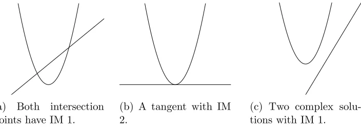
Here we want the weighted sum over the points of intersection to be two. There are three possible cases:
1. two points of intersection with IM one,
2. a single tangential intersection with IM two, or
3. two complex intersections with IM one.
In each case
2
p∈V(y−x2,y−ax−b)
im4p;y−x2, y
−ax−b5= 2
is satisfied. These cases are illustrated in Figure 3.1.
Regular points have intersection multiplicity one — in fact they can be defined by this property. Points at tangential intersections, crossovers, and singular points have IM greater than one. Everything else has IM zero.
(a) Both intersection points have IM 1.
(b) A tangent with IM 2.
(c) Two complex solu-tions with IM 1.
Figure 3.1: The various intersections of a line and parabola.
There are a myriad of ways to define the intersection multiplicity of two planar curves h0, h1 ∈ F[x, y]. Its ‘purest’ form is B´ezout’s
defini-tion which simply states a point’s intersecdefini-tion multiplicity is equal to the dimension of the local ring OA2(F), p at⟨h0, h1⟩.
Definition 3.1 (B´ezout’s IM for bivariates). Let h ⊆ F[x, y] and p ∈
V(h). Theintersection multiplicity ofp in V(h) is
im(p; h) := dim
vec(
bivariate intersection multiplicity 34
where OA2, p:=
Ff
g :f, g∈ F[x, y], g(p)̸= 0 G
.
As the intersection multiplicity is a local property it can safely be cal-culated using Taylor series instead of rational functions.
In order to different between ideal brackets and vector brackets we use⟨ ⟩
for the former and⟨⟨ ⟩⟩for the later. That is to say, when{f0, . . . , fe}⊆
F[x] then
⟨⟨f0, . . . , fe⟩⟩={c0f0+· · ·+cefe : c0, . . . , ce∈F}.
Example 3.1. Consider the parabola and line given by h = {y −x2,
y −x} ⊆ F[x, y] is x(x+ 1), y− x. Near 0, a point in h’s variety, we
have
F[[x, y]]/⟨h⟩=F[[x, y]]/⟨x(x+ 1), y−x⟩
(note (x+ 1) is a unit near0.) =F[[x, y]]/⟨x, y−x⟩
=F[[x, y]]/⟨x, y⟩
=⟨⟨1⟩⟩.
This means dimvec(OA2, p/⟨h⟩) = im(0;h) = 1.
Example 3.2 (Figure 3.1b). Consider the parabola and tangent line given by h={y−x2, y
}⊆F[x, y] is x2,y. Near 0we have
F[[x, y]]/⟨h⟩=F[[x, y]]/<y, x2=
={a+bx:a, b∈F}
=⟨⟨1, x⟩⟩.
fulton’s properties 35
§
3.2 Fulton’s Properties
Fulton’s constructive characterization of the intersection multiplicity is an an algorithm for planar curves. Indeed this algorithm, and its proofs, form the basis of our generalization.
The multiplicity of h ∈ F[x, y] at p (denoted mp(h)) is the tailing
degree of hwhen viewed as a polynomial from F[x−p].
Theorem 3.1 (Fulton’s Properties). Let two plane curves be given by h0, h1 ∈ F[x, y] and let p ∈ A2(F[x, y]). The intersection multiplicity of
h0, h1 atpsatisfies and is uniquely determined bythe following properties:
(2-1) im(p; h0, h1) =
⎧ ⎨ ⎩
∞ ifp ∈V(gcd(h0, h1))
n∈ N otherwise. ,
(2-2) im(p; h0, h1) = 0 ⇐⇒ p /∈V(h0)∩V(h1),
(2-3) im(p; h0, h1) is invariant to affine change of coordinates onA2(F),
(2-4) im(p; h0, h1) = im(p;h1, h0),
(2-5) im(p; h0, h1)≥ mp(h0)·mp(h1) with equality occurring if and only if
π
p(h0)!π
p(h1). That is, if V(h0) andV(h1) have no tangent linesin common at p,
(2-6) ∀g∈ F[x]; im(p; h0, h1) = im(p;h0, h1g)−im(p;h0, g), and
(2-7) ∀g∈ F[x]; im(p; h0, h1) = im(p;h0, h1+h0g).
Notice Theorem 3.1 classifies every point ofAℓ+14F5.
fulton’s properties 36
1 Function im(p; h0, h1)
Input:
1. p= (px, py)∈A2(F), and
2. h0, h1 ∈F[y≺x] : gcd(h0, h1)∈F.
Output: im(p; h0, h1)∈N satisfying (2-1)–(2-7).
2 if h0(p), h1(p)̸= 0 then 3 return0;
4 r, s←deg(h0(x, py)),deg(h1(x, py)); 5 if r > s then
6 returnim(p;h1, h0);
7 if r=−∞then /* (y−py)66h0(x, y) */
8 write h1(x, py) = (x−px)m(am+am(x−px) +· · ·); 9 returnm+ im(p; quo(h0, y−py; y), h1);
10 if r≤s then
11 h′1 ←h1−xs−r ℓc(h1(x, py))
ℓc(h0(x, py))
h0;
12 returnim(p;h′1, h0);
extending fulton’s properties 37
Example 3.3. Find the intersection multiplicity of h = {y, y−x2
} at the origin using Fulton’s algorithm. See Figure 3.1b for a geometric repre-sentation. Boxed values indicate the recursive calls and the remaining the algorithm’s trace.
line
im40;y, y−x25
(r, s)←deg40, 0−x25 4
= (−∞, 2)
h1(x, 0) =x2(−1) =⇒ m= 2 8
2 + im40; quo(y, y;y), y−x25
im40; 1, y−x25= 0 2
2.
Fulton’s algorithm has not yet been generalized to more than two hy-persurfaces.1 Moreover, Algorithm 2 is limited to computing intersection
multiplicities at rational coordinates from the base field. Thus, intersec-tion multiplicities at complex points, irraintersec-tional points, and more generally algebraic points cannot be calculated using this algorithm.
§
3.3 Extending Fulton’s Properties
Extending thegeometricdefinition of intersection multiplicity to more vari-ables is straightforward. We are still measuring the dimension of tangent spaces (albeit higher dimensional ones) about points in an affine space.
Definition 3.2 (B´ezout’s Intersection Multiplicity). Let h ⊆ F[x] and
p ∈V(h)⊆ Aℓ+14F5. The intersection multiplicity ofp in V(h) is
im(p; h) := dim
vec(
OAℓ+1, p/⟨h⟩).
extending fulton’s properties 38
OAℓ+1, p :=
Ff
g :f, g∈ F[x], g(p)̸= 0 G
.
Note that by [11, Chapter 4. §2 Proposition 11] we can substitute the power series ringF[[x−p]] forOAℓ+1, p/⟨h⟩below as they are isomorphic.
Example 3.4. Locally at the origin the system
h=0x, x−y2−z2, y−z31⊆F[x, y, z]
is x,y =z3,z2(z4+ 1). Near0 we have
F[[x]]/⟨h⟩=F[[x]]/<x, y−z3, z2=
=F[[x]]/<x, y, z2=
={a+bz :a, b ∈F}
=⟨⟨1, z⟩⟩,
where ⟨⟨1, z⟩⟩is a F-vector space. Thus im(0; h) = 2.
We propose, up to splitting, the following extension of Fulton’s prop-erties to correspond with Definition 3.2 for Regular Chains [24].
Theorem 3.2. Let h∈ S(F[x]) be a sequence inF[x] so that⟨h⟩is zero
dimensional, p := (p0, . . . , pℓ)∈ Aℓ+1
4F5
, and let h↓ denote the removal of the element hℓ∈h (i.e.,h={hℓ}∪h↓) then
im(p;h) satisfies (n-1) through (n-7)
where
(n-1) im(p; h)∈N,
(n-2) im(p; h) = 0 ⇐⇒ p̸∈V(h),
(n-3) im(p; h) is invariant to affine change of coordinates onAℓ+1(F),
(n-4) im(p; h) = im(p; σ(h)) for any permutation σ(h) of the elements of h,
(n-5) im(p; (x0−p0)m0, . . . ,(xℓ−pℓ)m
ℓ
extending fulton’s properties 39
(n-6) provided h↓, ghis a regular sequence (and thus dim
⟨h↓, gh
⟩ = 0)
im(p;h↓, gh) = im(p;h↓, g) + im(p; h↓, h),
(n-7) ∀g∈ ⟨h↓
⟩; im(p; h↓, h) = im(p;h↓, h+g).
For these seven properties, we adapt the proofs of [14, 18] and note all but (n-6) are trivial and (n-4) and (n-7) in particular are obvious because the intersection multiplicity depends only on p and ⟨h⟩.
Proof of (n-1). The sequence h is regular, so V(h) is proper intersection of varieties and⟨h⟩forms a zero dimensional ideal. The result follows.
Proof of (n-2). When p̸∈V(h).
p̸∈ V(h) =⇒ ∃f ∈ h:p ̸∈V(f) =⇒ f ̸∈ ⟨x−p⟩
=⇒ 1
f ∈ OAℓ+1, p =⇒ OAℓ+1, p/⟨h⟩=0
=⇒ dim
vec(
OAℓ+1, p/⟨h⟩) = dim
vec(0) = 0.
Conversely when p∈V(h).
p ∈V(h) =⇒ ∀f ∈h;f(p) = 0 =⇒ ⟨h⟩ ⊆ ⟨x−p⟩
=⇒ OAℓ+1, p/⟨x−p⟩ ⊆OAℓ+1, p/⟨h⟩
=⇒ dim
vec(
OAℓ+1, p/⟨x−p⟩)≤dim vec (
OAℓ+1, p/⟨h⟩).
As OAℓ+1, p/⟨x−p⟩is a field
dim
vec(
OAℓ+1, p/⟨x−p⟩) = 1
so it follows that
∀p∈V(h); dim
vec (