Dust Opacities
?Michiel Min
1Anton Pannekoek Institute, University of Amsterdam, The Netherlands
Abstract.Dust particles are the dominant source of opacity at (almost) all wavelengths and in (almost) all regions of protoplanetary disks. By this they govern the transport of energy through the disk and thus the thermal structure. Furthermore, their spectral prop-erties determine the low resolution spectral signature observed at infrared wavelengths. The infrared resonances that can be observed using low resolution infrared spectroscopy can be used to identify the composition and size distribution of the dust. The opacities depend on the size, shape, structure and composition of the particles, and computing them is not always trivial. In this chapter the ways in which the opacity of dust particles depend on the dust characteristics is discussed. Methods to compute them are outlined and the difficulties that can be encountered are addressed.
1 Introduction
Dust grains in cosmic environments obscure, scatter, and reprocess radiation. This means that a proper understanding of environments containing dust requires detailed knowledge of these processes. In addition, studying radiation that interacted with dust grains can teach us about the properties of the particles. In protoplanetary disks, dust grains are the main source of opacity at most wavelengths. They cause these disks to be heavily optically thick, and determine the radiation field and temperature structure in most parts of the disk. Thereby, they are also important for the dynamics of the disk.
The way in which dust particles interact with light depends on the dust particle characteristics like size, shape, and composition. Computations of the optical properties of dust particles thus require us to take these properties correctly into account. Unfortunately, this is not always feasible. Small scale substructure interior or at the surface of small grains require very high spatial resolution in the simulations that is usually not computationally feasible. Especially for large particles this becomes a significant issue, since it is required to both model the large scale structure of the particle, and the small scale substructure, since they can act on different aspects of the optical properties.
Laboratory measurements of the properties of cosmic dust grains are essential for understanding their optical properties for two important reasons. The first is that in all computations the first thing we have to know is the refractive index of the material. The wavelength dependent refractive index is very different for different material compositions and lattice structures. Therefore, measurements of the refractive index of a large set of materials relevant for cosmic dust is the essential first requirement for modeling any dusty structure. The second reason why laboratory measurements on cosmic dust
?4thLecture from Summer School “Protoplanetary Disks: Theory and Modelling Meet Observations”
are important is that our computational methods are limited, and it is essential that they are gauged by comparing to measured optical properties of realistic particles.
Over the past our understanding of how small particles interact with light has increased signifi-cantly. This topic is driven from many different fields of research. Many of the available computa-tional tools where developed for atmospheric research, biological research, or astronomy. However, also in industrial applications there is a large interest in this, for example in the paint industry, or the field of characterization of nano particles.
In this chapter we will focus on creating an understanding of the complexity of the problem, and what issues one has to think of. The purpose is to create awareness of the difficulties associated with the optical properties of dust particles and provide solutions to handle these issues properly when modeling or interpreting observations. Many of the insights and ideas discussed in this chapter come from the excellent books on this topic by Bohren & Huffman (1983); van de Hulst (1957) and from Draine (1988); Min (2009); Voshchinnikov et al. (2007) and other papers by these authors.
2 Interaction of light with a particle: the basics
The interaction of a light beam with a particle is usually divided into absorption and scattering. Ab-sorbed radiation can be transformed into thermal energy or used for chemical alteration or evaporation of the particle. Scattered radiation retains its original wavelength, but changes direction.
2.1 Interaction cross sections
We have to consider the effective cross sections for scattering and absorption of radiation. These quantities depend on the characteristics of the particle and on the wavelength of radiation. There are several quantities related to the cross sections of absorption, scattering, and extinction,Cabs,Csca, Cext=Cabs+Csca, that can be found in the literature. First there is the commonly used efficiency,
Qabs,sca,ext=Cabs,sca,ext
2πr , (1)
wherer is the size of the particle. This size is easily defined when the particle is a homogeneous sphere, but it becomes less transparent when the particle is irregularly shaped. In this case the size measure that is commonly used is thevolume equivalent radius,rV,
rV =
3V
4π
!1/3
, (2)
where V is the material volume of the particle, i.e. it is the radius of a sphere with the same material volume as the particle. There are two length scales involved in the scattering problem; the wavelength,
λ, and the size of the particle,rV. Therefore, it is convenient to use thesize parameter,
x=krV, (3)
wherek = 2π/λ. Due to scaling invariance of Maxwell’s equations, solutions with the same size parameter are equivalent.
Another commonly used quantity is the mass absorption, scattering, or extinction cross section,
κabs,sca,ext=Cabs,sca,ext
M , (4)
whereMis the total mass of the particle. This is the quantity we will mainly use in practice, since it has some nice properties as we will see later on.
Consider a monochromatic lightbeam traveling in a plane. We can divide the electric field into a component parallel to the plane,Ek, and a component perpendicular to the plane,E⊥. This light beam
can be fully represented by the Stokes vector,
S= I Q U V =
EkE∗k+E⊥E∗⊥ EkE∗k−E⊥E∗⊥ EkE∗⊥+E⊥E∗k i(EkE∗⊥−E⊥Ek∗)
. (5)
The intensity of the light wave is represented by the Stokes parameterI. The degree of linear po-larization is pQ2+U2/I, and the degree of circular polarization isV/I. The strength of the Stokes
vector becomes apparent when one wants to write down what happens when a light beam interacts with a particle. Upon interaction, the state of the light beam is changed. When we place a detector somewhere in the plane defined above, the scattered radiation detected due to interaction with the particle can be obtained through the scattering matrix,F,
I Q U V scat =
F11 F12 F13 F14 F21 F22 F23 F24 F31 F32 F33 F34 F41 F42 F43 F44
I Q U V inc . (6)
In principle the scattering matrix depends on the scattering angleθ, which is the angle between the incident and scattered direction, and azimuthal direction, i.e. the angle between the inertial frame of the particle and the scattering plane. The scattering matrix can not only be defined for a single particle, but also for a collection of particles. The scattering matrix simplifies significantly when the collection of particles obeys two simple rules: 1) they are in random orientation, and 2) for every particle the mirror particle exists. When this is the case, the scattering matrix becomes (van de Hulst 1957),
F=
F11 F12 0 0 F21 F22 0 0
0 0 F33 F34
0 0 −F34 F44 , (7)
so there are only 6 elements left. This assumption is often used in radiative transfer computations. Also, in this case the scattering matrix only depends on the scattering angle, i.e. the angle between incoming and scattered light, and no longer on the orientation of the scattering plane with respect to the inertial frame of the particle.
3 Computational methods
3.1 Mie theory
The simplest particle shape one can think of is that of a homogeneous sphere. The solution for the interaction of an electromagnetic wave with a homogeneous, spherical particle was first derived by Gustav Mie (Mie 1908). It is a very basic separation of variables technique, separating the angular and radial parts of Maxwell’s equations. For a derivation and the mathematical details please see e.g. Bohren & Huffman (1983). Mie theory provides a very stable method to compute the optical prop-erties numerically, and there are numerous codes available that do this in a robust way. The solution involves an infinite sum which converges typically afterN =|m|xterms, withmthe complex refrac-tive index of the material andxthe size parameter. Thus, Mie theory becomes more computationally challenging for large particles, small wavelengths, or highly conducting materials.
The termMie theoryorMie scattering, is widely used in the literature to also refer to the solution for a radially stratified sphere, since the solution method is basically the same. It is even sometimes, erroneously, used for interaction of any type of particle with size comparable to the wavelength of radiation.
3.2 Rayleigh approximation, small particles
When the particle is much smaller than the wavelength of radiation both inside and outside the particle, i.e. x1 and x|m| 1, the problem simplifies significantly. In this case, we can assume that the incoming electric field is homogeneous over the extend of the particle, the so-called electrostatic approximation. A particle will respond to this homogeneous electric field like a single ideal dipole. The dipole moment induced by the applied electric fieldEis given by (for a derivation see Chapter 5 of Bohren & Huffman 1983),
p=αEinc, (8)
whereαis the polarizability, i.e. the ease with which the particle is polarized. The cross sections for absorption and scattering can be directly derived from the polarizability,
Cabs=kIm(α), (9)
Csca= k4
6π|α|
2. (10)
There are exact solutions for the polarizability of only a few particle shapes; spheres, ellipsoids, and layered spheres. The polarizability of an ellipsoid with the electric field applied along one of the axis is given by,
α=V m
2−1
1+L(m2−1), (11)
with 0<L<1 the form factor of the ellipsoid, depending on the axes ratios of the three different axes. There are three different form factorsL1,2,3 for the field applied along the different axes of
the ellipsoid. The form factor has the property thatL1+L2+L3 = 1. For a homogeneous sphere L1=L2=L3=1/3 and the polarizability becomes,
α=3Vm 2−1
m2+2. (12)
It now also becomes clear why it is convenient to use the mass absorption cross section,κabs. In the
limit of very small particles, the cross section,Cabs, is proportional to the volume of the particle, and
Up to now we have only considered the case where the particle is composed of a single material with refractive indexm. In practice, however, this is often not the case. There are numerical methods that can solve for complex systems with multiple materials (like the DDA discussed below), but a first order method to treat mixtures of materials is through theeffective medium theory. In effective medium theory it is assumed that the mixing of materials takes place on the smallest possible scales, such that at any resolution one only observes an effective refractive index, meff. In this way the
computational methods for single material particles can again be applied.
Consider an infinite medium with refractive indexmmwhich we will call the matrix material. The
polarizability of a small spherical inhomogeneity with refractive indexmiin that medium is given by,
αi=3V(mi/mm) 2−1
(mi/mm)2+2
. (13)
Now the two most commonly used effective medium theories state that the polarizability of the eff ec-tive medium inside this matrix material is the average of the polarizabilities of the materials that make up the medium,
(meff/mm)2−1
(meff/mm)2+2
=X
i
wi(mi/mm)2−1
(mi/mm)2+2
, (14)
wherewiis the volume fraction of materiali. To solve formeff, the quantity which we want to derive,
we have to define what the matrix material,mm, is. In the Garnett mixing rule one choses the dominant
material in the mixture, somm =mj. This makes it possible to write down a closed form solution of
Eq. 14, and is a good approximation if one wants to look at the effects of small abundance polutions in a material. In the Bruggeman mixing rule one makes the logical choice thatmm=meff (so the left
hand side of Eq. 14 becomes zero). This makes physically more sense, but also makes it more difficult to solve formeff. In practice however, a simple iterative scheme usually converges relatively fast. Note
that using effective medium theory one can also quite easily add porosity to the particles by including a material withmi=1.
It is good to realize the assumptions that go into effective medium theory. The most important one is that the mixing takes place at the smallest possible scale. For aggregates composed of constituents of different materials, this condition is obviously violated, since the constituents have finite size. Also, the assumption is that the inhomogeneities are spherical. This can have effects on the shapes of spectral resonances (see e.g. Min et al. 2008, for a discussion and proposed solution for this problem).
3.4 Discrete Dipole Approximation (DDA)
When we consider the particle to be build up from a large collection of very small sub-units, each of which interacts with the local electric field as a single dipole, we have (Draine 1988)
pj=αj
Einc,j− N
X
k,j
Ajkpk
, (15)
wherepjis the local dipole moment at the position of sub-unit j,αjis the polarizability of sub-unit
j,Einc,jis the incoming field at the location of sub-unitj, andNis the total number of sub-units. The
3×3 matrixAjkdetermines the electric field at the position of sub-unitjdue to the dipole field emitted
by sub-unitk(Draine 1988).
Ajkpk=
exp(ikrjk)
4πr3
jk
n
(kri j)2rˆjk×(ˆrjk×pk)+
1−ikrjk I3−3ˆrjkrˆjk
pk
o
where ˆri j is the unit vector pointing from dipoleito dipole j,ri j is the distance between these two
dipoles,I3is the 3×3 identity matrix, and the 3×3 matrix ˆri jrˆi jis defined as the product of ˆri jas a
column vector and ˆri jas a row vector, i.e.
ˆ
ri jrˆi j=
ˆ r2
i j,x rˆi j,xrˆi j,y rˆi j,xrˆi j,z
ˆ
ri j,xrˆi j,y rˆi j2,y rˆi j,yrˆi j,z
ˆ
ri j,xrˆi j,z rˆi j,yrˆi j,z ˆri j2,z
, (17)
where ˆri j,x,rˆi j,yand ˆri j,zare thex, yandzcomponents of the unit vector ˆri j, respectively. It is clear that
Eqs. 15 and 16 can be conveniently written as a single matrix equation.
˜
Einc=
˜
A+B˜p˜, (18)
where the ˜Einc and ˜p are 3N vectors containing the vectorsEinc,j andpj for all values of j, ˜Ais a
3N×3Nmatrix containing the matricesAi jfor alli,j, and ˜Bis a diagonal matrix with the values of α−1
j on the diagonal. When this is solved for ˜p(and thus forpj) the absorption cross section is given
by,
Cabs=
4πk
|Einc|2
N
X
j=1 (
Imhpj·(α−1j )
∗ p∗ji−2
3k
3 p∗j·pj
)
, (19)
where the asterisks denote the complex conjugates. In the same way the other optical properties can be derived from thepj(Draine 1988).
3.4.1 DDA in the Rayleigh approximation
In the limit of very small particles, i.e. very long wavelengths, Eq. 16 simplifies significantly,
Aij=
I3−3ˆri jrˆi j
4πr3
i j
, i, j, (20)
which makes ˜A real and symmetric. When we also assume the particle is homogeneous, i.e. ˜
B=α−1I3
N, the solution forpjcan be written directly in terms of the eigenvalues and eigenvectors
of ˜A. The derivation of this is beyond the scope of this chapter, but is relatively straightforward and elegant and the interested reader is referred to Min et al. (2006b) for all details. The final result is that the cross section of any particle of any shape can be written as a sum over the so-called form-factor distribution,
Cabs= 3N
X
j=1
wj
"
kVIm m
2−1
1+Lj(m2−1)
!#
, (21)
Here the values ofwjare obtained from the eigenvectors of ˜A, and the form-factorsLjfrom its
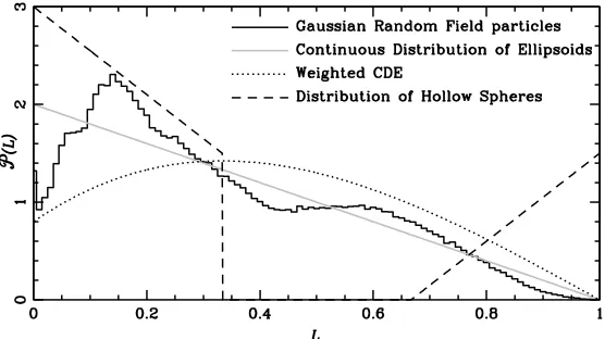
Figure 1.The form-factor distributions for different particle shape models used in the literature. Shown are the curves for irregularly shaped Gaussian Random Field particles (Min et al. 2007), the Continuous Distribution of Ellipsoids (CDE Bohren & Huffman 1983), a weighted version of CDE (see e.g. Li 2008), and the Distribution of Hollow Spheres (DHS; Min et al. 2005).
In Fig. 1 a few form factor distributions are shown for different particle shapes. What is immedi-ately clear is that there is almost always a strong contribution from very low value ofL. These low values ofLcorrespond to extremely flattened or elongated ellipsoidal particles. This is not because the aspect ratio of the original particles is very high, but it represents sub-structure on the particle which has this behavior.
3.5 The statistical approach
The main idea of the statistical approach is to simplify the computation of optical properties but at the same time use a framework which is able to reduce the resonances introduced by oversimplifying the computations (for example by using homogeneous spherical particles). This idea was made popular by Bohren & Huffman (1983) by introducing the so-called Continuous Distribution of Ellipsoids (CDE) for the analysis of infrared spectra (see also below).
As we have seen in the previous section, in the Rayleigh domain the absorption properties of any particle can be represented by those of a collection of ellipsoidal particles. This strongly supports the more general idea that the optical properties of a complex particle can be represented by those of a properly chosen collection of simple shapes. This has great computational advantages, since the optical properties of simple particle shapes can be computed much more efficiently. In addition, it allows a more strict focus on the particle characteristics that can be obtained from the observations.
Classically, spheroids have been a commonly used particle shape for applying the statistical ap-proach (e.g. Dubovik et al. 2006; Fabian et al. 2001; Mishchenko et al. 1997, and many others). However, as discussed in the previous section, the aspect ratio that one has to use to reproduce the observed particle properties does not always represent the true particle shape. It can be that high as-pect ratios are needed (lowLvalues) to reproduce rough surface substructure of an overall relatively spherical particle.
a hollow sphere will not tempt anyone in interpreting the true particle shapes directly from the fitted distribution. Actually, the fact that DHS provides such a good fit to many observational properties of cosmic dust grains is an argument in itself that this interpretation of particle shapes should be done with great care.
In the DHS shape distribution we simply average over the fraction f occupied by the central vacuum inclusion in the particle from zero to some value fmax≤1, giving equal weights to all values
of f while the material volume of the particle is kept the same. This means that the particles with higher values of f have a larger outer radius. Thus a particle with f=0 represents a homogeneous, solid sphere, while f≈1 represents a large, very thin bubble. The distribution is given by
n(f)=
1/fmax, 0≤ f < fmax,
0, f ≥ fmax,
(22)
wheren(f)d f is the fraction of the number of particles in the distribution betweenf andf+d f. The statistical approach has been often applied for spectroscopic analysis of solid state resonances. For this, usually particles much smaller than the wavelength dominate the spectra. Therefore, we can apply the Rayleigh limit. One of the most commonly used distributions of particle shapes is the Continuous Distribution of Ellipsoids. This is basically a form factor distribution with,
w(L)=2−2L, 0<L<1. (23)
The resulting absorption cross section is,
CabsCDE=2kVIm m
2
m2−1lnm 2
!
. (24)
CDE has been extremely successful in fitting infrared spectra of various mineralogical components in protoplanetary disks and dust around evolved stars and comets. Also for DHS with fmax=1 there is a
closed form solution forCabsin the Rayleigh limit (Min et al. 2003),
CDHSabs =3kVIm 2m
2+1
2m2−2 ln
"(2
m2+1)(m2+2) 9m2
#!
. (25)
4 Refractive index data
There are generally speaking two different ways to obtain the refractive index of a material: 1) from reflection spectra of polished bulk material, and 2) from transmission spectra of a powder. The first method is direct and the most accurate. However, this is not always available for all materials. The second method requires a model for the particles to invert the powder spectrum into a refractive index spectrum, and this is far from unique. Therefore, it is crucial to check how the refractive index data one uses is obtained before applying different particle shape models to it.
0.1 1.0 10.0 100.0 1000.0
λ [µm] 0.001
0.010 0.100 1.000 10.000
refractive index
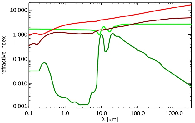
Figure 2. Laboratory measurements of the refractive index of silicate (green curves) and carbonaceous (red curves) materials (data from Dorschner et al. 1995; Zubko et al. 1996). The light red and green curves are the real part of the refractive index, the dark red and green curves the imaginary parts.
into their lattice. This makes for a less well-defined lattice, and the way in which the material was formed can now become important for the exact optical properties.
A very good place to start when looking for the optical properties of a large selection of cos-mic dust materials is the database of measurements performed in Jena: http://www.astro.uni-jena.de/ Laboratory/OCDB/.
As an example in Fig. 2 the refractive index of amorphous magnesium rich pyroxene and amor-phous carbon are plotted as a function of wavelength.
For spectral resonances of crystalline materials, it is often useful to consider a theoretical oscillator model for the refractive index. Solid state features in crystalline materials are usually well described by the Lorentz oscillator model (see e.g. Bohren & Huffman 1983). This model considers the refrac-tive index due to harmonic lattice vibrations. The eigenfrequency of the harmonic oscillator isω0. If
there is only one eigenfrequency (resonance) this gives a refractive index
m2=m20+ ξω 2
p ω2
0−ω2−iγω
. (26)
In this equationm0 is the real valued refractive index forω → ∞,ξis the oscillator strength of the
feature,ωpis the plasma frequency,ωis the frequency of incident radiation andγis a damping factor.
Ifωis expressed in wavenumbers, we can express Eq. (26) in wavelengths by usingω=λ−1. If there
are multiple eigenfrequencies,m2 is a sum over different values ofξ, ω
0 andγ. This model is used
quite successfully, for example, for obtaining the refractive index from reflectance data.
0.1 1.0 10.0 100.0 1000.0
λ [µm] 100
101
102
103
104
105
κ
[cm
−
2 /g]
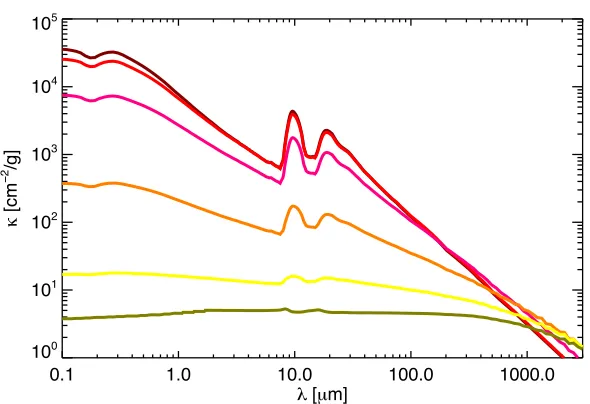
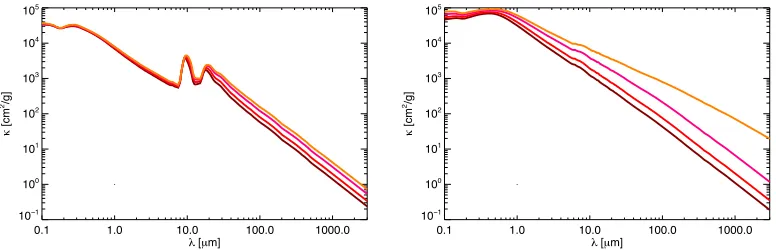
Figure 3. Mass absorption cross sections for a size distribution of particles with different slopes. The curves representp=5.0,4.5,4.0,3.5,3.0,2.5 for the maroon, red, pink, orange, yellow, and olive curves respectively.
properties (Cabs,Csca,F) over the three different crystallographic axes. DDA is one of the few methods
that actually provides a natural way of dealing with material anisotropy.
5 General dependence on particle properties
The optical properties of a particle depend on the particle characteristics. Here we will discuss the general dependencies on particle size, material, and shape. Note that by shape we also refer to internal structure of the particle. The computations presented below are all based on the DIANA standards, as discussed in section 7. For understanding the dependencies the computational details are at this point not needed.
5.1 Size dependence
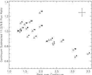
Figure 4. The strength of the 10µm silicate feature versus the shape for a selection of observed disks around Herbig stars. The strength on the x-axis is measured as the peak over continuum, while the shape, represented by the continuum subtracted flux at 11.3 and 9.8µm, is a measure for the broadness of the band. The figure is taken from (van Boekel et al. 2005, reproduced with permission cESO), and the reader is referred to that paper for details on the exact definition of the quantities.
all particle properties are kept the same, but we skew the size distribution towards smaller or larger particle sizes. The effects this has will be discussed below.
The size distribution used in Fig. 3 is given by
n(r)dr∝
r−p, r
min<r<rmax,
0, elsewhere (27)
where we fix the minimum and maximum size of the distribution tormin=0.05µm,rmax=3000µm.
The curves correspond to different values of p, and thus to different weight of the small and large particle component (decreasing values ofpcorrespond to increasing weight of the large particles).
There are a few size indicators frequently used in the literature:
1. The solid state features 2. The anisotropy of scattering 3. The slope of millimeter emission 4. The degree of linear polarisation
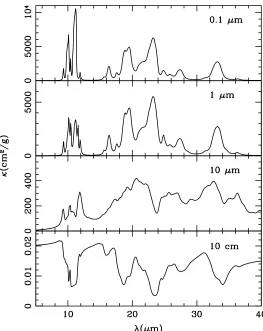
Figure 5.The mass absorption cross section for forsterite particles of different sizes. The computations are done using the DHS shape distribution. The weakening, and eventual inversion of the solid state resonances is clearly seen. Figure taken from Min (2009).
0 50 100 150 scattering angle θ[ο
] 10−1
100
101
102 103
104
105 10
F11
[cm
2 /g/sr]
rV = 0.2 µm
rV = 0.4 µm
rV = 1.2 µm
rV = 2.0 µm
rV = 4.0 µm
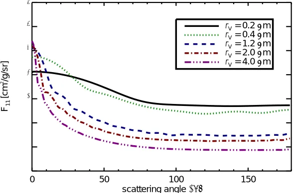
Figure 6. The phase function,F11for particles of different sizes. The computations are performed using DHS withfmax=0.8.
at smaller values ofxthen for wavelengths away from the resonance. Thus the net effect is that the spectral resonance decreases in strength.
With the above explanation it is easy to understand that very strong resonances, i.e. those with high values of|m|, will be affected by this for smaller particle sizes, as will spectral resonances at shorter wavelengths. This dependence of the spectral resonances on intrinsic feature strength and spectral location can be used to estimate particle sizes made up of crystalline material (see also Fig. 5 from Min et al. 2004). The complex dependence of the absorption cross section on size and refractive index also causes the 10µm amorphous silicate feature to broaden when the particle size increases. This broadening and weakening is an often used diagnostic to identify grain growth (for example see Fig. 4 from van Boekel et al. 2005).
The anisotropy of scattering: Very small particles scatter light in all directions almost isotrop-ically. When the particle size increases, the scattering becomes increasingly forward peaked (see Fig. 6). Spatially resolved images of scattered light from a protoplanetary disk can therefore be used to determine particle sizes. The difference between the part of the disk tilted towards us and the part of the disk tilted away from us can be used to estimate the anisotropy of the scattering phase function (at least in the range of angles probed by the geometry of the system). This is commonly done for spatially resolved debris disks, which are optically and geometrically thin, making this analysis trivial. For protoplanetary disks the vertical extend of the disk (which is often unknown) and the effects of op-tical depth, make the analysis less straightforward. One has to be careful when relating the anisotropy of scattering observed in a limited range of scattering angles to a particle size. Where computational methods using smooth particles will give a generally good idea on the scattering anisotropy over the entire range of scattering angles, it can be different for realistic particles at intermediate to backward scattering angles. This will be discussed in more detail in the section on aggregates.
0.1 1.0 10.0 100.0 1000.0
λ [µm] 0.1
1.0 10.0 100.0 1000.0
κ
[cm
2 /g]
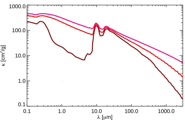
Figure 7. Mass absorption cross section as a function of wavelength for different mixtures of materials. The maroon, red, and pink curves correspond to 0, 13, and 25 % amorphous carbon material by mass.
of disturbance of the incoming electromagnetic wave. It becomes increasingly forward peaked when increasing the geometrical shadow of the particle. For truly macroscopic objects it becomes so heavily forward peaked that it is not recognized as scattering anymore, since it basically does not alter the path of the incoming light beam, which is why for these bodies we only have to consider reflection.
The slope of millimeter emission: The absorption cross section of particle at millimeter wave-lengths can usually be characterized relatively well by a single powerlaw,
Cabs∝λ−β (28)
For dielectric (i.e. non conducting) particles much smaller than the wavelength we haveβ=2. For conducting materials, like for example graphite, iron sulfide or metallic iron, the value ofβis usually much smaller. In the interstellar medium the value ofβ≈1.7 (Draine 2006). When the particle size increases, the value ofβdecreases. For protoplanetary disks values ofβbetween 0.1 and 1.8 have been reported (see e.g. Lommen et al. 2010). These low values ofβare usually attributed to particle growth, but can also be partly explained by an increased amount of e.g. graphitic material. To see the change in slope when the grain size increases we plot in Fig. 3 a mixture of carbonaceous and silicate materials with a changing size distribution. The effect of adjusting the abundance of carbonaceous material is visualized in Fig. 7. Here it is very clear that an increasing amount of carbon can have a significant impact making the millimeter slope much shallower.
The degree of linear polarisation: Particles in the Rayleigh domain are very efficient polarizers. The provide a degree of linear polarization which is 100 % at 90◦ scattering. As the grain size
Figure 8. The 10µm amorphous silicate feature for different compositions of the silicate. Figure taken from (Min et al. 2007, reproduced with permission cESO).
this corresponds to a scattering angle ofθBrew=π−2 arctan(m). For silicate material in the optical part
of the spectrumm≈1.6, i.e.θBrew≈64◦. At this angle a smooth surface spherical particle will display
100 % polarization. For other smooth surface convex particles this angle can be slightly different, but will always exist. However, when the surface is not smooth, the polarization will be imperfect and much lower, like what is detected for realistic particles in the laboratory, but also from rough surface scattering (i.e. the polarization phase curve of atmosphereless solar system bodies). The conclusion is that there is certainly potential in using the degree of polarization, but that using it requires very careful modeling of particle shape and surface structure. We will return to the topic of polarization when discussing aggregate particles.
5.2 Material dependence
Different materials display different spectral structure in the opacities. Details in the location and width of solid state features can be attributed to differences in material properties. For example the 10µm amorphous silicate feature is very dependent on the exact composition of the silicate (see Fig. 8). Also, the more general behavior in the optical part of the spectrum can be very different. Amorphous silicates with only magnesium in the lattice have a very low absorption efficiency, while the inclusion of a small amount of iron atoms can boost the absorption significantly. This is very important for the heating of cosmic dust particles.
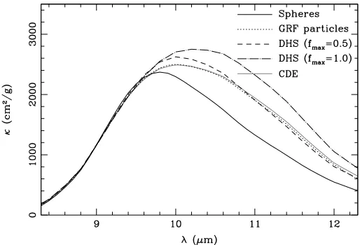
Figure 9.The shape of the 10µm silicate feature for different particle shape distributions. We plot the feature for homogeneous spheres, Gaussian Random Field (GRF) particles (see Min et al. 2007, for details), DHS particles with different values offmax, and CDE. The shift and broadening of the feature for increasing deviations of perfect spherical particles is very clear. Figure taken from (Min et al. 2007, reproduced with permission cESO).
5.3 Shape dependence
Particles of different shapes produce different opacities. The simplest shape one can consider is that of a homogeneous sphere, for which the full solution of Maxwell’s equations is easily written down. However, a homogeneous sphere has been shown to be a poor representation of cosmic dust particles in general (e.g. Fabian et al. 2001). The main reason for this is that a perfect sphere exhibits resonances that do not occur in nature. A commonly heard remark is that a size distribution will wash out these resonances. However, although a size distribution might mask the resonances by smoothing them, they do not go away.
The most important effects of particle shape are seen when the refractive index is relatively high. In these cases particle shape becomes a crucial parameter. This manifests itself in two important aspects: the solid state features, and the millimeter opacity of conducting materials.
Solid state features are locations in the spectrum where the refractive index locally increases. As can be seen from Eq. 11 the maximum absorption efficiency of an ellipsoid depends on the value of
L. Since the refractive index at the spectral location of a feature rapidly changes, it goes through all different values, and thus crosses the different maxima for different values ofL. This means that the exact location of the solid state resonance is a strong function ofL(or the shape of the form-factor distribution). This effect is strongest for the very strong resonances found for crystalline materials, but it is also very clear for amorphous silicates (see Fig. 9).
Conducting (or semi-conducting) materials can be considered as materials with a spectral reso-nance atω0=0 (or very small values of ω0; see Eq. 26). Thus at long wavelengths the refractive
index increases towards relatively high values. This implies that, similar to the shape dependence of the spectral resonances, the millimeter slope of these materials becomes highly dependent on particle shape. This is illustrated in Fig. 10 where we plot the absorption efficiencies for a standard mixture of silicate and carbon, and for pure carbon grains for different values of fmax. Due to the use of
0.1 1.0 10.0 100.0 1000.0
λ [µm]
10−1
100
101
102
103
104
κ
[cm
2/g]
0.1 1.0 10.0 100.0 1000.0
λ [µm]
10−1
100
101
102
103
104
κ
[cm
2/g]
Figure 10. Mass absorption cross sections as a function of wavelength for different values of the irregularity parameter in the DHS shape distribution. Left figure shows a standard silicate carbon mixture, while right figure is for pure carbon grains. Maroon, red, pink, and orange curves correspond tofmax=0,0.4,0.8,1.0 respectively.
(the carbon abundance is relatively low), thus the millimeter opacity slope is not heavily influenced. However, for the pure carbon grains, the slope in the millimeter changes significantly when fmaxis
increased. Amorphous carbon is still a semi-conducting material, i.e. its refractive index does not reach extreme values. If we would consider more extreme materials, like metallic iron, these effects are even stronger.
The difficulty with this strong dependence on particle shape is that it is impossible to exactly model the particle shapes that we expect. The small scale substructure is essential, so only considering the external shape of the particle (which is usually rather simpel, or even spherical) is not enough. However, how strong the effects of substructure really are is a question that has no simple answer. The best solution for this is to consider laboratory measurements of powder materials and fit these using a shape distribution. This has been done by Mutschke et al. (2009), who fitted a form-factor distribution to measurements of powder spectra. These powder spectra are also well represented by a DHS shape distribution with fmax≈0.8. For very high refractive indices the maximum absorption cross section
is obtained for extremely low values of the form-factorL. Thus, for computations of these materials, the detailed shape of the form-factor distribution at these very lowL-values is crucial. However, these extremely high refractive indices are usually not probed by solid state spectral resonances. Thus, a model that reproduces the solid state spectral resonances very well is not automatically successful at representing the optical properties of (semi)conducting materials at millimeter wavelengths (see also Fig. 2).
6 General properties of aggregates
Kimura et al. (2006); Min et al. (2006a); Volten et al. (2007) and DDA computations of aggregate particles from Min et al.in prep.
Kataoka et al. (2014) discuss the opacity evolution of very fluffy aggregates with particle size and filling factor using effective medium theory. They conclude that for very fluffy aggregates the absorption (and thus emission) properties of aggregates are determined by the factor f·r, with f
the filling factor andrthe outer radius of the aggregate. Aggregates with the same f·rvalues have the same mass absorption cross section. For scattering, this is somewhat different and the interested reader is referred to their paper for details. They also provide an analytical formula for the opacities of aggregate particles, which should be used with care, as one of the main assumptions going in is the assumption that the monomers are perfect spheres, which influences among others the millimeter slope when conducting materials are present.
6.1 The solid state features
The 10µm silicate feature of aggregates of different fractal dimension was studied in detail by Min et al. (2006a). The conclusion of this study is that for the same aggregate mass (so the samerV)
the feature is stronger when the fluffyness of the aggregate is increased (i.e. its fractal dimension is decreased). Fig. 11 (taken from Min et al. 2006a) displays this very clearly. The way to understand this is that the particle needs to become ’optically thick’ for the feature to decrease in strength. Since the average density of a very fluffy aggregate is much lower than for a compact aggregate with the same mass, its optical depth is also smaller. Note here that we can use the concept of optical depth only as a way to understand this effect. The interaction of light with a particle should strictly be described in terms of the Maxwell equations, and only for very large particles this can be done using radiative transfer concepts.
6.2 The anisotropy of scattering and degree of linear polarisation
As discussed above, for very large particles scattering is made up of a diffraction term and a reflection term. The scattering phase function of aggregate particles can be understood from these two terms qualitatively. Since the diffraction term only depends on the size of the geometrical shadow, it is not dependent on the exact shape of the particle but only on the external size of the aggregate as a whole. This term causes an increasing forward scattering with increasing aggregate size. At intermediate to backscattering angles the scattering of a large particle is dominated by reflection. However, for an aggregate particle the substructure caused by the monomers of the aggregate is crucial, so we cannot consider this part of the scattering as reflection offa smooth surface. This part of the scattering term is caused by the monomers of the particle and the ’surface’ they create. Computations and labora-tory measurements show that this part of the scattering is indeed dominated by the properties of the monomers of the aggregate (e.g. Volten et al. 2007). This implies that also the degree of linear polar-ization at intermediate scattering angles is completely dominated by what the monomers do. Compare this to the polarization behavior of very large smooth particles, displaying 100 % polarization around the Brewster angle, and it is clear that this can be very different (see also Fig. 12 taken from Min et al.
in prep).
7 DIANA standards
Figure 11.The 10µm absorption spectra of aggregate particles for different volume equivalent radii. The solid curves show the computations for the aggregate particles, the dotted curves for homogeneous spheres with the same size, and the dashed curves display a porous sphere approximation. The upper panels show graphical representations of the aggregates withrV=2µm, the bar below the aggregates displays a measure for the scale
of the image by showing the diameter of a volume equivalent sphere. Figure taken from (Min et al. 2006a, reproduced with permission cESO).
aggregates
0 50 100 150
θ[ο ] 10−1 100 101 102 103 104 105 106 F11 r V = 0.2 µm rV = 0.4 µm
r V = 1.2 µm rV = 2.0 µm
r V = 4.0 µm
aggregates at λ = 0.55 µm
0 50 100 150
θ[ο ] −0.1 0.0 0.1 0.2 0.3 0.4 0.5 0.6
degree of polarization rV = 0.2 µm
r V = 2.0 µm rV = 4.0 µm
Figure 12.Phase function,F11(left), and polarization curve,−F12/F11(right), computed for aggregate particles of different sizes.
7.1 Dust size distribution
For the dust size distribution we take a simple powerlaw with minimum size rmin =0.05µm and
maximum sizermax=3000µm according to Eq. 27 with the power of the powerlaw,p, a free parameter.
7.2 Dust shape distribution
We choose to adopt the Distribution of Hollow Spheres, DHS Min et al. (2005). This has the advantage that computations can be carried out quite efficiently and the accuracy of the computations is greatly enhanced with respect to perfect spheres. The DHS has one shape parameter, which is the maximum volume fraction of the inner vacuum cavity,fmax.
7.3 Composition
The composition of the grains is taken to be a mixture of amorphous silicates and amorphous carbon. All other components are not included in the standard setup. Even though iron sulfide is a very likely component of protoplanetary dust, for simplicity we assume the optical properties of all featureless components are well represented by a single continuum opacity source which we take to be amor-phous carbon. For the interpretation of the results, this has to be kept in mind, the amoramor-phous carbon represents all unknown, featureless opacity sources.
In addition to these two materials, we mix in a fraction of vacuum, to simulate porosity. We take 25% of the volume to be vacuum, which is a rather mild porosity. Among others, this influences the strength of the 10 micron silicate feature.
We mix everything together using the Bruggeman mixing rule (Eq. 14 withmm=meff), which can
be written as,
N
X
i=1
wi m
2
i −m
2 eff m2
i +2m
2 eff
=0, (29)
To mix in vacuum, one has to simply mix in a material withmi=1. The Bruggeman effective medium
which also favors Mg rich silicates. We follow the composition of interstellar silicates as derived by Min et al. (2007), which has Mg/(Mg+Fe)≈0.7. For simplicity we only consider the pyroxene stoichiometry.
The refractive index data we take from
• Silicate: Mg0.7Fe0.3SiO3from Dorschner et al. (1995) (material densityρ=3.01 g/cm3)
• Carbon: from Zubko et al. (1996), sample BE (we take the material densityρ=1.80 g/cm3)
There are several studies reporting on refractive index data for carbonaceous material. The refrac-tive indices are often different, which can be attributed to different lattice structures of the carbon. The choice of the carbon material we propose comes from the following considerations. First, the data has to be smooth, featureless. Second, conducting materials like carbon, graphite, iron sulfide, or metallic iron, have increasing refractive index at long wavelengths. This heavily influences the mm slope of the opacities. However, this effect is not visible in all measurements of amorphous carbon, but we want to select one that does. These considerations are very practical, i.e. the data has to be able to reproduce our observations.
Towards wavelengths shorter than available from the measurements, one could in principle ex-trapolate using the equations given by Bohren & Huffman (1983, page 234)
n=1− ω
2
p
2ω2, k=
γω2
p
2ω3, (30)
withnandkthe real and imaginary part of the refractive index. The parametersωpandγare obtained from the first datapoint available. However, we find that for the materials we use, this does not give a logical extrapolation. Therefore, we take the refractive index to be constant for the small range we have to extrapolate towards smaller wavelengths.
For wavelengths longer than available from the measurements, we use a loglog extrapolation. We decide not to use the general extrapolation formula for dielectrics since this is inaccurate for semi-conducting materials like carbon.
The carbon fraction determines in part the strength of the silicate feature and greatly influences the opacity slope at millimeter wavelengths. We take this to be a free parameter in the modeling. Useful values are between 10 and 20% by mass. An important characteristic influenced by the amount of carbon is the slope of the mm opacity,β. This varies fromβ=1.8 for 5% carbon toβ=1.4 when using 20% carbon for the smallest grain sizes. The value ofβis also influenced by grain size (decreasing with increasing grain size).
7.4 Summary of the standards
When modeling protoplanetary disks, there are parameters of the dust grains that we want to vary, and parameters that we want to fix. We fix the shape distribution and materials we use, while the size distribution and carbon content are parameters that we can vary.
For the particle shape we use the DHS model. We include porosity and mix the materials into one effective material using the Bruggeman mixing rule. All fixed and free parameters are summarized in Table 1.
8 Summary
Table 1.The parameters used for the standardized optical properties used in the DIANA modeling framework. The parameter ranges given for the free parameters are only indications of reasonable values.
fixed parameters
minimum size (rmin) 0.05µm
maximum size (rmax) 3000µm
irregularity parameter (fmax) 0.8
vacuum fraction (wvac) 0.25 (by volume)
optical data used Silicate (ρ=3.01 g/cm3), Mg
0.7Fe0.3SiO3 Dorschner et al. (1995)
Carbon (ρ=1.80 g/cm3), sample BE Zubko et al. (1996)
free parameters
powerlaw (p) ≈2.5 to 4.5
carbon fraction (wcarbon) ≈10 to 20% by mass
above how these dependencies work in general, and where one has to be extra careful in drawing conclusions. We describe an approach into computing optical properties for protoplanetary dust that takes into account most of these considerations, and provides a starting framework for studies of dust in protoplanetary disks.
The wealth of complications arising when computing optical properties have in the past discour-aged people from using anything different than the most simple approach. We hope to have provided enough insight into this complex problem to provide handles into deviating just enough from this oversimplified approach and to use appropriate approximations and insights to arrive at more robust and balanced conclusions.
AcknowledgementsThe research leading to these results has received funding from the European
Union Seventh Framework Programme FP7-2011 under grant agreement no 284405.
References
Bohren, C. F. & Huffman, D. R. 1983, Absorption and scattering of light by small particles
Dorschner, J., Begemann, B., Henning, T., Jaeger, C., & Mutschke, H. 1995, A&A, 300, 503
Draine, B. T. 1988, ApJ, 333, 848
Draine, B. T. 2006, ApJ, 636, 1114
Dubovik, O., Sinyuk, A., Lapyonok, T., et al. 2006, Journal of Geophysical Research (Atmospheres), 111, 11208
Fabian, D., Henning, T., Jäger, C., et al. 2001, A&A, 378, 228
Kataoka, A., Okuzumi, S., Tanaka, H., & Nomura, H. 2014, A&A, 568, A42
Kimura, H., Kolokolova, L., & Mann, I. 2006, A&A, 449, 1243
Mie, G. 1908, Annalen der Physik, 330, 377
Min, M. 2009, in Astronomical Society of the Pacific Conference Series, Vol. 414, Cosmic Dust -Near and Far, ed. T. Henning, E. Grün, & J. Steinacker, 356
Min, M., Dominik, C., Hovenier, J. W., de Koter, A., & Waters, L. B. F. M. 2006a, A&A, 445, 1005
Min, M., Dominik, C., & Waters, L. B. F. M. 2004, A&A, 413, L35
Min, M., Hovenier, J. W., & de Koter, A. 2003, A&A, 404, 35
Min, M., Hovenier, J. W., & de Koter, A. 2005, A&A, 432, 909
Min, M., Hovenier, J. W., Dominik, C., de Koter, A., & Yurkin, M. A. 2006b, J. Quant. Spec. Ra-diat. Transf., 97, 161
Min, M., Hovenier, J. W., Waters, L. B. F. M., & de Koter, A. 2008, A&A, 489, 135
Min, M., Waters, L. B. F. M., de Koter, A., et al. 2007, A&A, 462, 667
Mishchenko, M. I., Travis, L. D., Kahn, R. A., & West, R. A. 1997, J. Geophys. Res., 102, 16831
Mutschke, H., Min, M., & Tamanai, A. 2009, A&A, 504, 875
van Boekel, R., Min, M., Waters, L. B. F. M., et al. 2005, A&A, 437, 189
van de Hulst, H. C. 1957, Light Scattering by Small Particles
Volten, H., Muñoz, O., Hovenier, J. W., et al. 2007, A&A, 470, 377
Voshchinnikov, N. V., Videen, G., & Henning, T. 2007, Appl. Opt., 46, 4065